Identification of Single-Blade Angle Variation in Axial Flow Pumps Based on the Variational Mode Decomposition Method

Abstract

Pressure pulsations are crucial data within the flow field of a pump, and the characteristics of these pulsations can reveal changes in the internal flow. Based on model experiments, this paper obtained pressure pulsation data under two blade conditions and compared direct time-domain observations, peak-to-peak value changes, and the VMD decomposition method. The results show that even when it is known that one blade condition has changed, it is not possible to determine this through direct observation of pressure pulsation changes. The peak-to-peak value changes indicate that under special flow conditions, they are easily affected by different operating conditions, which can interfere with the results. In contrast, the VMD method, which decomposes the signal into low-frequency components, can better display anomalies within the pressure pulsation cycle and is less susceptible to the interference of flow conditions, offering some reference significance for diagnosing the blade operating conditions of the main pump.

1. Introduction

Axial flow pumps, a type of fluid machinery widely used in water conservancy projects and industrial systems, are extensively utilized in large-scale axial flow pump stations along rivers and coasts to serve irrigation and drainage functions [1,2,3,4]. They also play a significant role in inter-basin water transfer. The efficient and stable operation of axial flow pumps is crucial for the reliability of the entire system [5]. Due to the rotation of the impeller blades in the pump, pressure pulsations, which are important parameters for observing the internal flow characteristics of the pump, are generated internally.

Research on the pressure pulsations of hydraulic machinery mainly falls into two categories. One category focuses on studying the impact of different parameters on the pulsation characteristics of hydraulic machinery. Shi et al. [6] conducted numerical simulations and experimental studies on the differences in pressure pulsations between full tubular pumps and conventional axial flow pumps, finding that under low-flow conditions, the pressure pulsations of full tubular pumps are greater than those of conventional axial flow pumps. Spence et al. [7] monitored the pressure pulsations at a series of points on a centrifugal pump and found that monitoring the pulsations at the stop point on the pump volute is more representative. Fu et al. [8] used one-dimensional and three-dimensional coupled compressible flow simulation methods to perform numerical calculations on the load rejection process of ultra-high head prototype pump-turbine units, pointing out that other low-frequency components of pressure pulsations are caused by the unstable transition of flow separation and backflow vortices near the high-pressure inlet of the impeller, and the unstable transition of flow patterns in the impeller of ultra-high head prototype pump-turbines may lead to high-amplitude pressure pulsations, while stable vortex structures do not cause significant pressure pulsations. Lu et al. [9] utilized wavelet analysis and fast Fourier transform to analyze the pressure fluctuations at the inlet and outlet of centrifugal pumps caused by cavitation, obtaining the onset of cavitation and the emergence of unstable cavitation points in centrifugal pumps. They also employed dynamic mode decomposition to decompose the internal flow field of the centrifugal pump, gaining insights into the mechanism of pressure fluctuations caused by steady-state cavitation. Song et al. [10] found that when floor-attached vortices occur under high-flow conditions, the time-domain characteristic curve of pressure pulsations is significantly disturbed, and the amplitude of pressure pulsations changes significantly with the position of the floor-attached vortices. These studies mainly use changes in pressure pulsations to judge changes in the internal flow state of the pump, further revealing the impact of parameter changes on pump performance.

The other category of research focuses on reducing the amplitude of pressure pulsations within the pump to reduce its impact. Cao et al. [11] analyzed the pressure pulsations of a cycloidal pump with and without pulsation-damping at different speeds, with the highest reduction in pulsations being about 9.8%. Zhang et al. [12] reviewed the pressure pulsations within the pump and mentioned that methods such as increasing the rotor-stator gap, staggered blades, and blade modification can effectively reduce pressure pulsations. Zhang et al. [13] proposed a method of controlling the trailing edge parameters of the runner blades, and through optimized design, the relative pressure pulsation intensity in the draft tube was significantly reduced. Wang et al. [14] studied the influence of the relative position of the centrifugal pump diffuser on the main frequency and the amplitude of the decomposed frequency of pressure pulsations. The comparison of the amplitude of the main frequency of pressure pulsations showed that when the trailing edge of the diffuser is at the left corner of the volute outlet, the transient pressure on the volute has the lowest pulsation. Binama et al. [15] used numerical simulation methods to study the influence of the blade trailing edge hub position on the pressure field characteristics of the centrifugal PAT under part-load conditions, and different PAT models showed different pressure pulsation characteristics. Trivedi et al. [16] investigated the unsteady pressure fluctuations in two prototype Francis turbines during load variation and start-up and found that the amplitude of synchronous pressure pulsation is much larger than that of asynchronous pressure pulsation.

In recent years, signal analysis methods have been increasingly applied to the analysis of hydraulic performance of hydraulic machinery. Sonawat et al. [17] used the fast Fourier transform (FFT) to calculate the amplitude of pressure pulsations of a double-suction centrifugal pump and found that a combination of a 30-degree staggered design and a split volute can transmit the smallest pressure pulsations. Lu et al. [9] used the dynamic mode decomposition method to decompose the pressure pulsation characteristics under quasi-steady cavitation in a centrifugal pump, and the results showed that different inlet states lead to obvious differences in internal flow and unsteady flow structures. Zhang et al. [18] used the dynamic mode decomposition method to study the unsteady flow structure inside a centrifugal pump and analyzed the mechanism of pressure pulsations. The unstable flow inside the impeller is mainly affected by the inlet state, system rotation, and impeller structure, and the research is helpful for the design of centrifugal pumps. Fang et al. [19] introduced an optimization method combining Long Short-Term Memory (LSTM) and Variational Mode Decomposition (VMD) to enhance the prediction accuracy of pressure pulsation signals of reversible pump-turbines. Ren et al. [20] proposed a denoising method based on the Sparrow Search Algorithm (SSA)-optimized VMD combined with Singular Value Decomposition (SVD), which has certain application significance for the extraction and fault diagnosis of pressure pulsations in pumped storage units. Zhou et al. [21] studied the pressure pulsation characteristics under the load rejection condition of the pump-turbine and proposed a new denoising method that can better extract water disturbance pressure, which has certain engineering significance. Zhang et al. [22], based on the VMD method, analyzed the pressure pulsation characteristics of the pump-turbine, and the results showed that the bladeless area and the guide vane area show the same characteristics of each part, that is, strong low-frequency fluctuations and a wide frequency domain, and the fluctuation frequency components are mainly the blade frequency and its multiples in the bladeless area.

This paper is based on the test of pressure pulsation data under two blade conditions. It analyzes the performance and pulsation characteristics of the pump, extracts the characteristic distribution of different blade conditions through the VMD method, identifies the change in blade state, and analyzes the impact of blade state change on the pressure pulsation characteristics, providing reference for the blade state diagnosis of axial flow pumps and the safe operation of pump stations.

2. Test System and Method

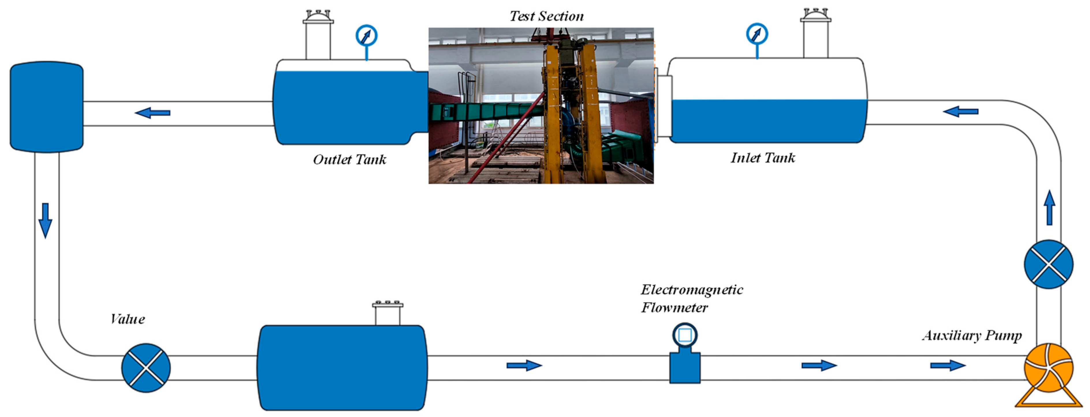
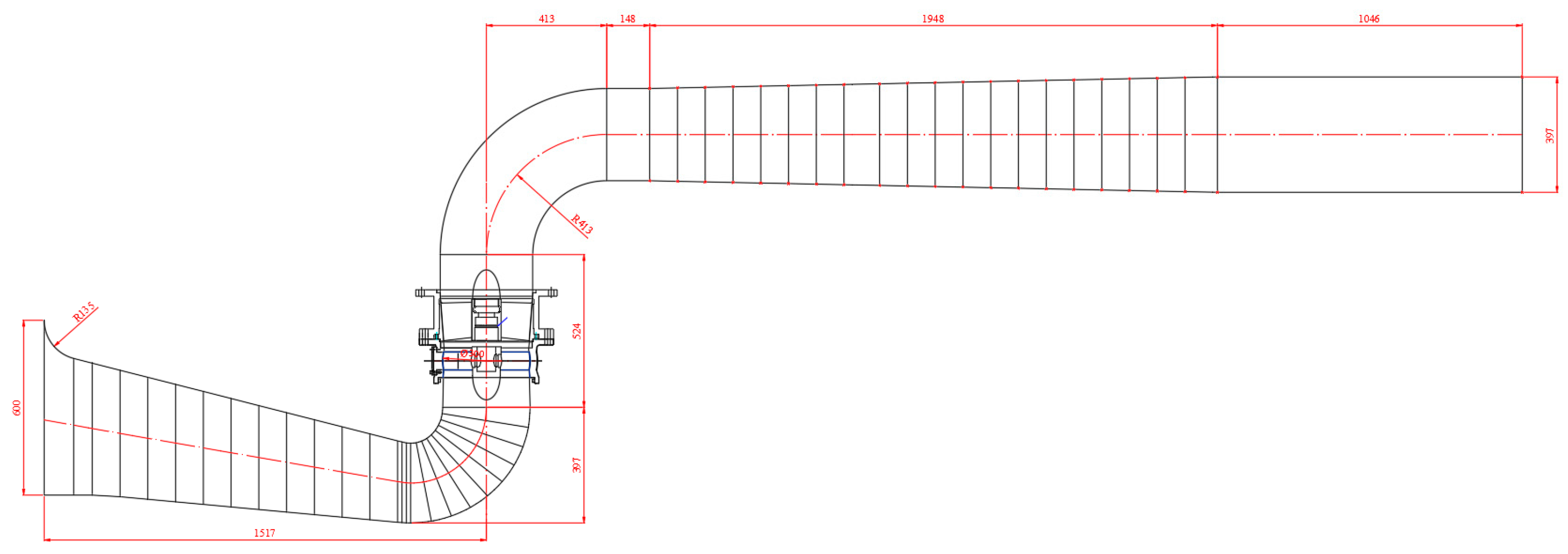
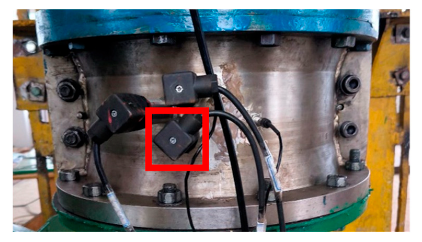
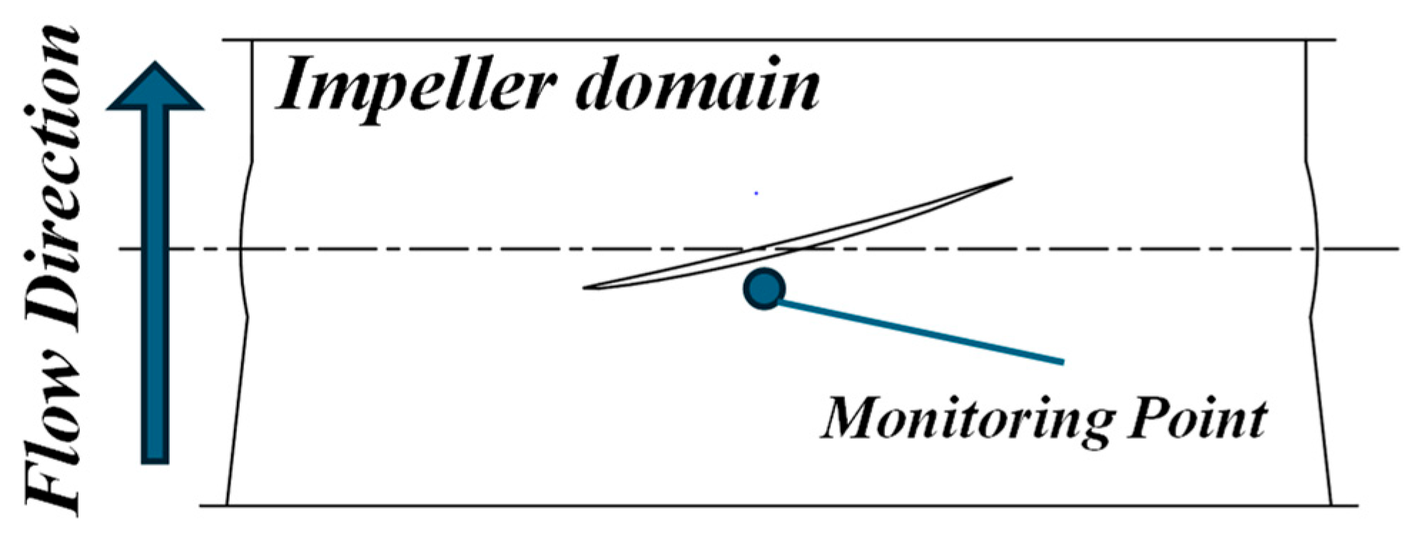
2.1. Model Test

The test was conducted on the high-precision hydraulic machinery test bench at Yangzhou University. The schematic diagram of the test rig is shown in Figure 1. The test rig is a closed-loop system that controls the flow rate through auxiliary pumps and gates to change the test conditions. The performance of the pump system is obtained through testing instruments, as shown in

Table 1. Measuring instruments and their attributes.

Measurement Item	Measuring Instrument	Equipment Name	Working Range	Calibration Accuracy
Head	Differential Pressure Transmitter	EJA110A	0~100 kPa	±0.1%
Flow rate	Electromagnetic Flow Meter	E-mag	0~500 L/s	±0.2%
Torque Speed	Torque Speed Sensor	JC2C	500 N·m	±0.15% ±0.05%

. A schematic diagram of the model pump system is shown in Figure 2, and the impeller diameter is 300 mm. The main technical parameters of the test bench and pump unit are shown in

Table 2. Technical parameters of test bench and pump system.

Test Bench		Pump System
Volume	50 m3	Design head	4.75 m
Flow rate	0~2160 m3/h	Design flow rate	1278.7 m3/h
Power	0~80 kW	Maximum efficiency	76.6%
Pressure	30 kPa~150 kPa	Design power	21.57 kW

.

The total uncertainty of the efficiency of the test is

$$\begin{array}{c}{E}_{\eta }=\pm \sqrt{{\left(E_{\eta }\right)}_s^2+{\left(E_{\eta }\right)}_r^2}=0.370\%\end{array}$$

(1)

where $(E_{\eta }{)}_r$ is the random uncertainty,

$$\begin{array}{c}(E_{\eta }{)}_r=\pm {\displaystyle \frac{t_{0.95\left(N-1\right)}\times S_{\stackrel{-}{\eta }}}{\stackrel{-}{\eta }}}\times 100\%\end{array}$$

(2)

and $S_{\stackrel{-}{\eta }}$ means standard deviation of the efficiency test, based on the test results, and $(E_{\eta }{)}_r=0.25\mathrm{\%}$. $(E_{\eta }{)}_s$ is the system uncertainty, determined according to the measurement accuracy of the measuring instrument, which is 0.273%.

The pressure pulsation measurement points are located on the impeller’s periphery, as shown in Figure 3. The red box in the figure is the pressure pulsation measurement point at the leading edge of the impeller. Generally, the pressure pulsations at the leading edge of the blade have the most significant amplitude and are the most characteristic; hence, only the measurement results at the leading edge are analyzed. The approximate positions of the measurement points and the blades are shown in Figure 4. In the experiment, the blades are divided into a normal condition (NOR), where all blade angles are consistent, and a condition with one blade angle change (OBAC).

2.2. VMD Method

Variational Mode Decomposition (VMD) is an adaptive signal decomposition method that can decompose nonlinear and non-stationary signals into a series of inherent oscillation modes, which are localized in both frequency and time. The principle of the VMD method is based on the variational principle, obtaining the inherent oscillation modes of the signal by minimizing an energy function. According to Equations (3) and (4), a constrained variational problem is constructed.

$$\begin{array}{c}\underset{u_k,{\omega }_k}{\mathrm{m}\mathrm{i}\mathrm{n}}\left\{{\sum }_k\parallel {\partial }_t\left[\left(\delta \left(t\right)+{\displaystyle \frac{j}{\pi t}}\right)u_k\left(t\right)\right]e^{-j{\omega }_{k}t}{\parallel }_2^2\right\}\end{array}$$

(3)

$$\sum _k{u}_k=f$$

(4)

In the formulas, $u_k$ is the modal component; $f$ is the original signal; $t$ is the time window; $\delta \left(t\right)$ is the Dirac distribution about time t; ${\omega }_k$ is the center frequency of each modal component; $e^{-j{\omega }_{k}t}$ is the estimated center frequency of each analytical signal; $k$ represents the decomposed mode index; $j$ represents the unit imaginary number.

In the solution to the aforementioned formulas, a quadratic penalty factor and the Lagrange multiplier are introduced, leading to the Alternating Direction Method of Multipliers (ADMM) for obtaining the updated formulas for the modes and their sums, namely Equations (5) and (6):

$$\begin{array}{c}{\widehat{u}}_k^{n+1}\left(\omega \right)={\displaystyle \frac{\widehat{f}\left(\omega \right)-{\sum }_{i\ne k}{u}_i\left(\omega \right)+\frac{\widehat{\lambda }\left(\omega \right)}{2}}{1+2\alpha {\left(\omega -{\omega }_k\right)}^2}}\end{array}$$

(5)

$${\omega }_k^{n+1}={\displaystyle \frac{{\int }_{\mathrm{\infty }}^0\omega {\left|{\widehat{u}}_k\left(\omega \right)\right|}^{2}d\omega }{{\int }_{\mathrm{\infty }}^0{\left|{\widehat{u}}_k\left(\omega \right)\right|}^{2}d\omega }}$$

(6)

where ${\widehat{u}}_k^{n+1}\left(\omega \right)$ represents the Weiner filter equivalent to the current residual $\widehat{f}\left(\omega \right)-{\sum }_{i\ne k}{u}_i\left(\omega \right)$, and ${\omega }_k^{n+1}$ is the centroid of the power spectrum of the current intrinsic mode. Equation (5) is used to update ${\lambda }^{n+1}$:

$$\begin{array}{c}{\mathsf{\lambda }}^{n+1}={\mathsf{\lambda }}^n+\tau \left[f\left(\mathsf{\omega }\right)-{\displaystyle \sum _k}{u}_k^{n+1}\right\}\end{array}$$

(7)

3. Results and Discussion

Figure 5 illustrates the external characteristics of the axial flow pump under different blade conditions. When there is a change in the angle of one blade, it significantly affects the performance of the pump. At high-flow and design-flow conditions, the changes in pump performance are the most pronounced, with a maximum decrease of about 9.4% in head and about 3.5% in efficiency. However, under low-flow conditions, the changes are relatively minor, with the head slightly lower than in the normal condition, and the efficiency remaining essentially the same. We selected the pressure pulsation conditions at the leading edge of the blade under three flow conditions for analysis, with the selected conditions indicated by the green circles in the figure. The low-flow condition is approximately 0.8 Qd, the design-flow is Qd, and the high-flow condition is 1.2 Qd.

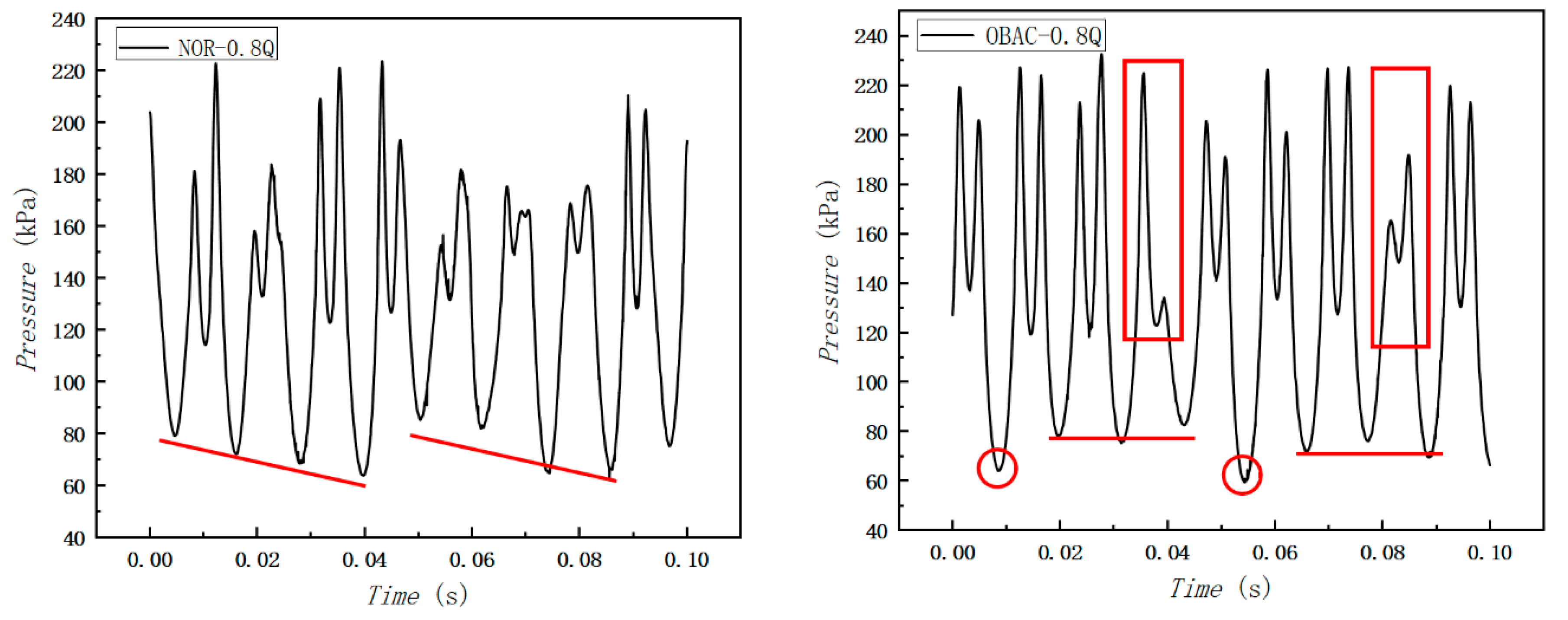
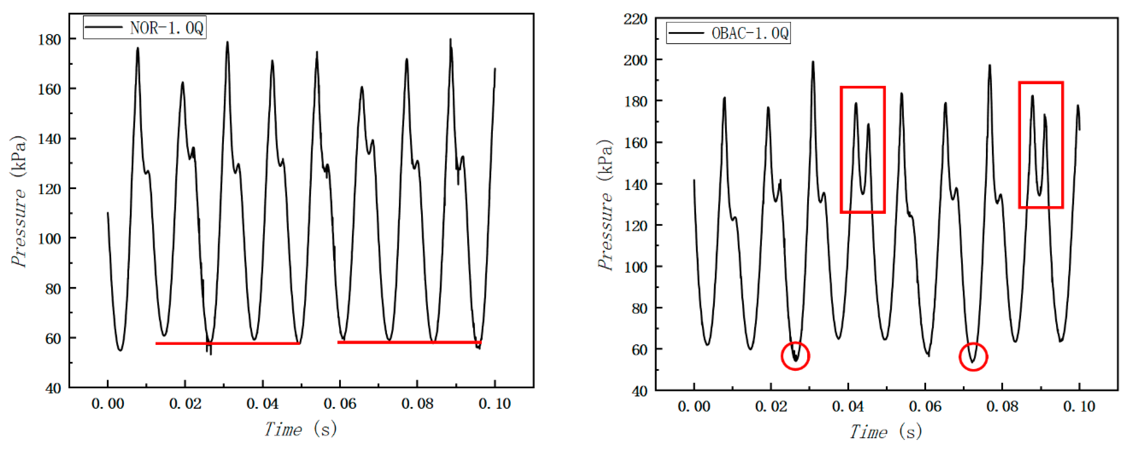
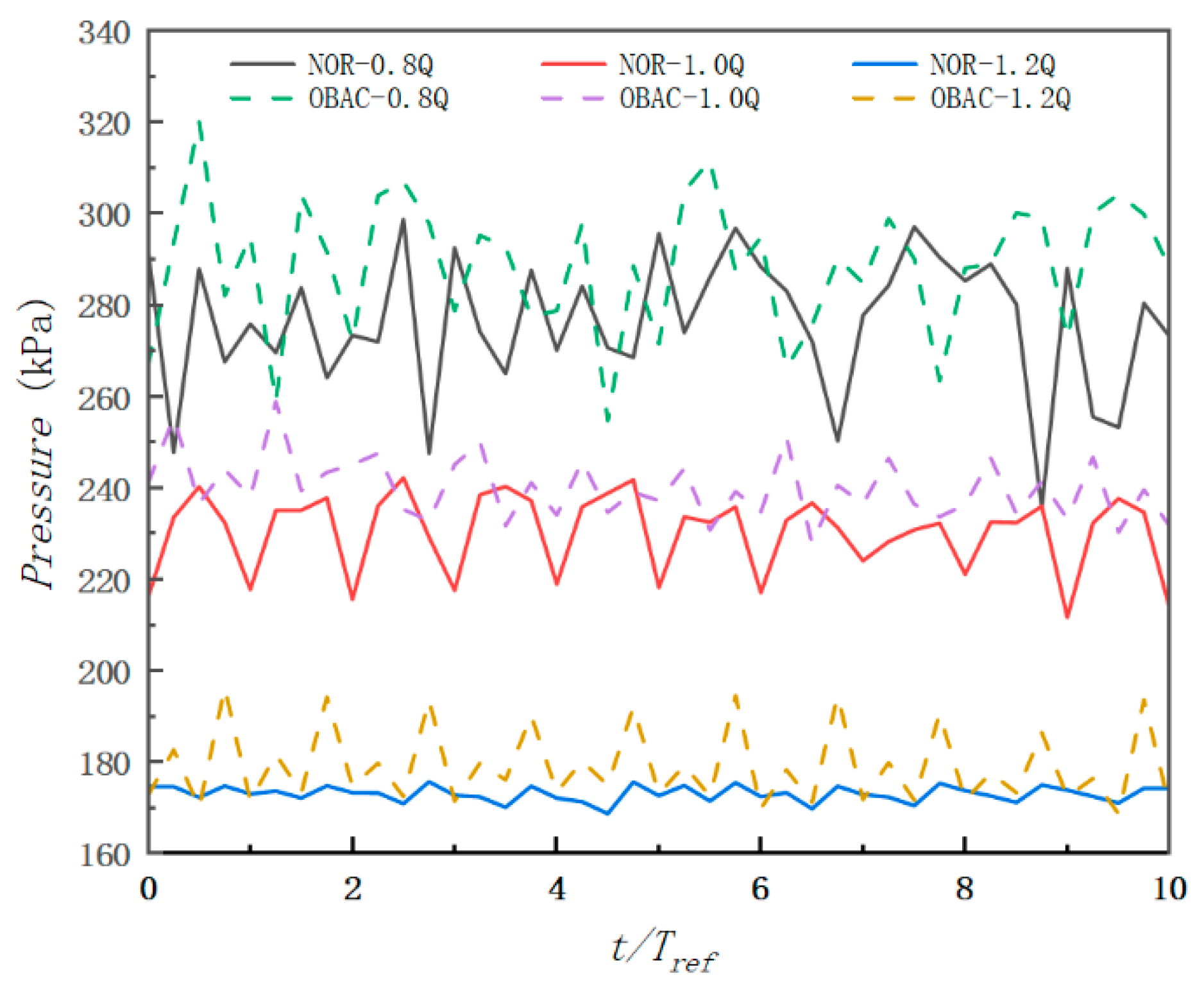
3.1. Pressure Pulsation Time-Domain Analysis

When the angle of one blade changes, theoretically, there should be a noticeable difference in the time domain of the pressure pulsation, as shown in Figure 6, Figure 7 and Figure 8, which display the time domain of the pressure pulsation under different flow conditions for the two blade states. The blade rotation speed is 1300 r/min, the time period is approximately 0.04615 s, and the number of blades is four, meaning that every four waves constitute a cycle.

At 0.8 Q, under the NOR condition, the low-pressure troughs show a nearly linear trend, with the maximum difference between the two troughs being about 20 kPa. The high-pressure peaks exhibit a secondary peak, and the peak values do not show a clear trend. Under the OBAC condition, a significant minimum value can be observed in the trough, while the values of the other three troughs are not much different, with the maximum difference also close to 20 kPa. The peaks also show a secondary peak, with one peak being different from the others, showing two significantly different peak values. It is observed that the abnormal positions of the peaks and troughs do not occur on the same wave, meaning they are not caused by the same blade.

At the 1.0 Qd condition, the pressure pulsation changes are much more stable. Under the NOR state, the wave heights and shapes produced by different blades in the pressure pulsation are essentially consistent, and the signal is relatively stable. However, under the OBAC state, abnormalities in both peaks and troughs are observed, similar to the low-flow condition, and they are not caused by the same blade.

At the 1.2 Qd condition, the pressure pulsation waveform is similar to that at the design-flow rate. Under high-flow conditions, the pressure pulsation waveform is simpler. In the NOR state, the pulsation is stable, and the waveforms are similar to each other. In the OBAC state, the waveform is not as uniform as in the NOR state, with abnormal values appearing in the wave troughs, while the peaks exhibit a linear trend.

Based on the observations of pressure pulsation, even when it is known that the angle of one blade has changed, it is difficult to clearly distinguish the changed blade from the time-domain diagram alone. Additionally, abnormalities in peaks and troughs may not occur on the same wave, making it challenging to determine whether the blade angle has truly changed.

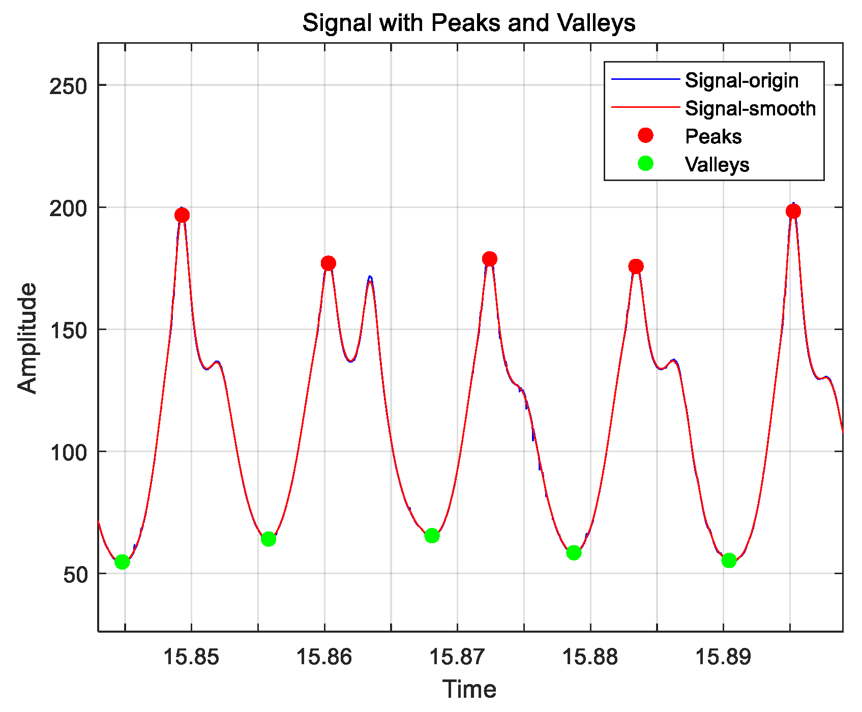
3.2. Peak-to-Peak Value Variation

To clearly perceive the differences between the blades, we extracted the peak-to-peak values of the pressure pulsations for observation. Initially, the peak-to-peak data were smoothed to avoid local spike data affecting the judgment results. A peak-finding algorithm was used to determine the positions of the peaks and troughs, and a specific peak-finding interval width was designated. Figure 9 shows the effect of the smoothed data compared to the original data, also displaying the positions of the peaks and troughs.

Figure 10 presents the results after processing the peak-to-peak values. The horizontal axis represents the number of cycles, with four peak-to-peak values within a cycle. According to the results, under the 0.8 Qd condition, there is a significant fluctuation in the peak-to-peak values regardless of the blade condition, with no clear periodic pattern. Under the 1.0 Qd condition, both blade states exhibit periodicity; the NOR condition has a minimal peak-to-peak value within each cycle, while the other three peak-to-peak values are relatively consistent. The reason for this situation may be due to manual adjustments of the blade angle, resulting in a significant deviation in the angle of one blade, which should be around ±0.5°, much smaller than 2°, but the change in peak-to-peak values is quite apparent. The OBAC condition, on the other hand, shows an extreme value in contrast to the NOR condition, with the peak-to-peak value variation being significantly smaller. Only under high-flow conditions can the differences between the two blade states be more clearly distinguished, with the NOR condition showing a more stable peak-to-peak variation, while the OBAC condition exhibits a noticeable extreme value.

The method of using peak-to-peak values to determine the blade state also has certain issues. Only under high-flow conditions can the differences be clearly observed; other conditions do not allow for determining whether there is a problem with the blades.

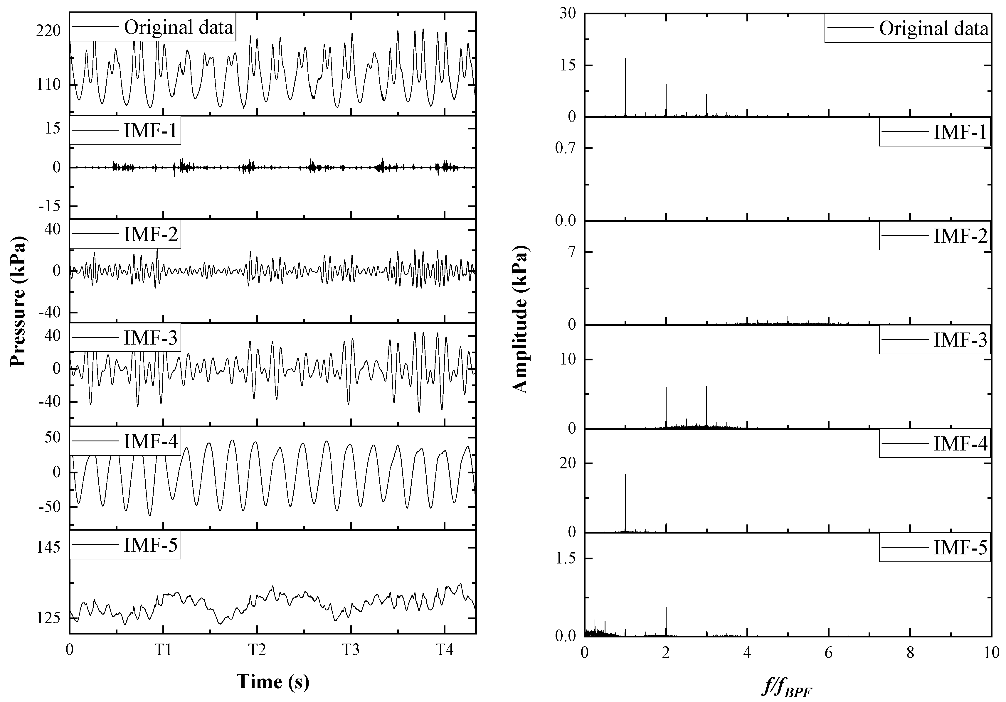
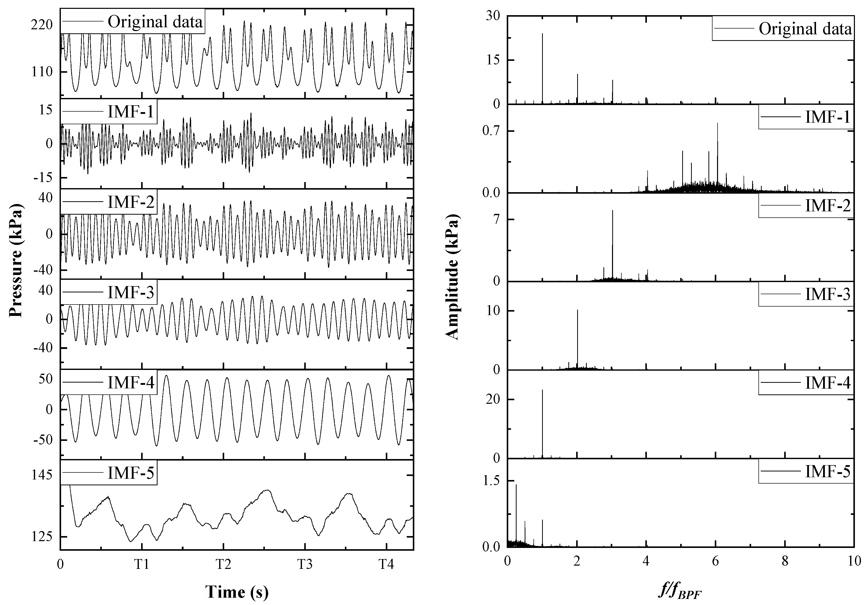
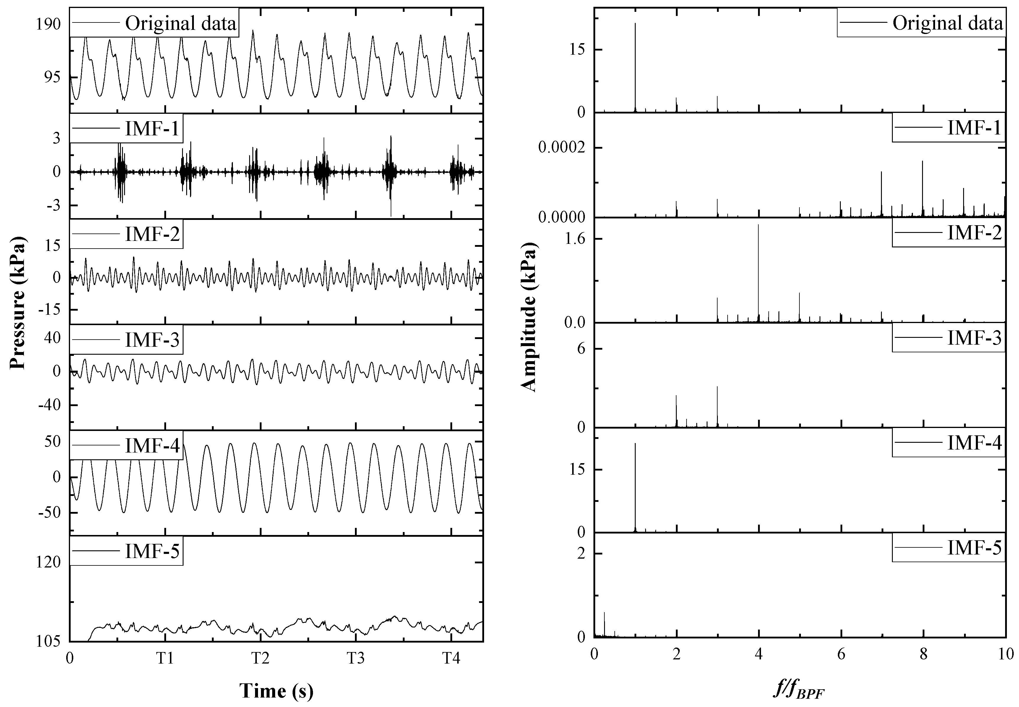
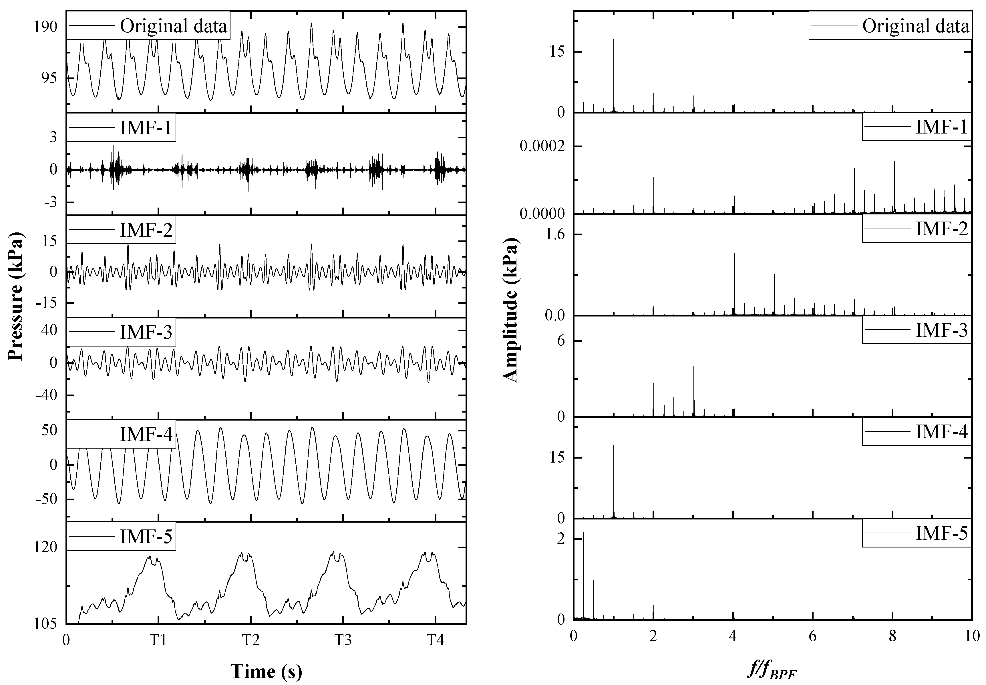
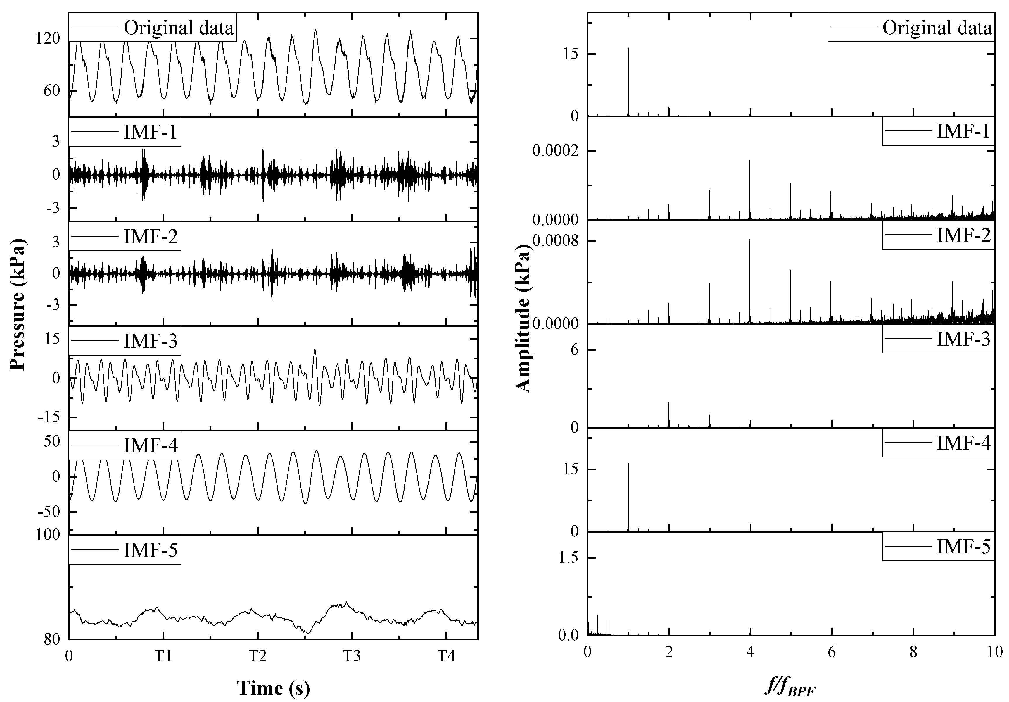
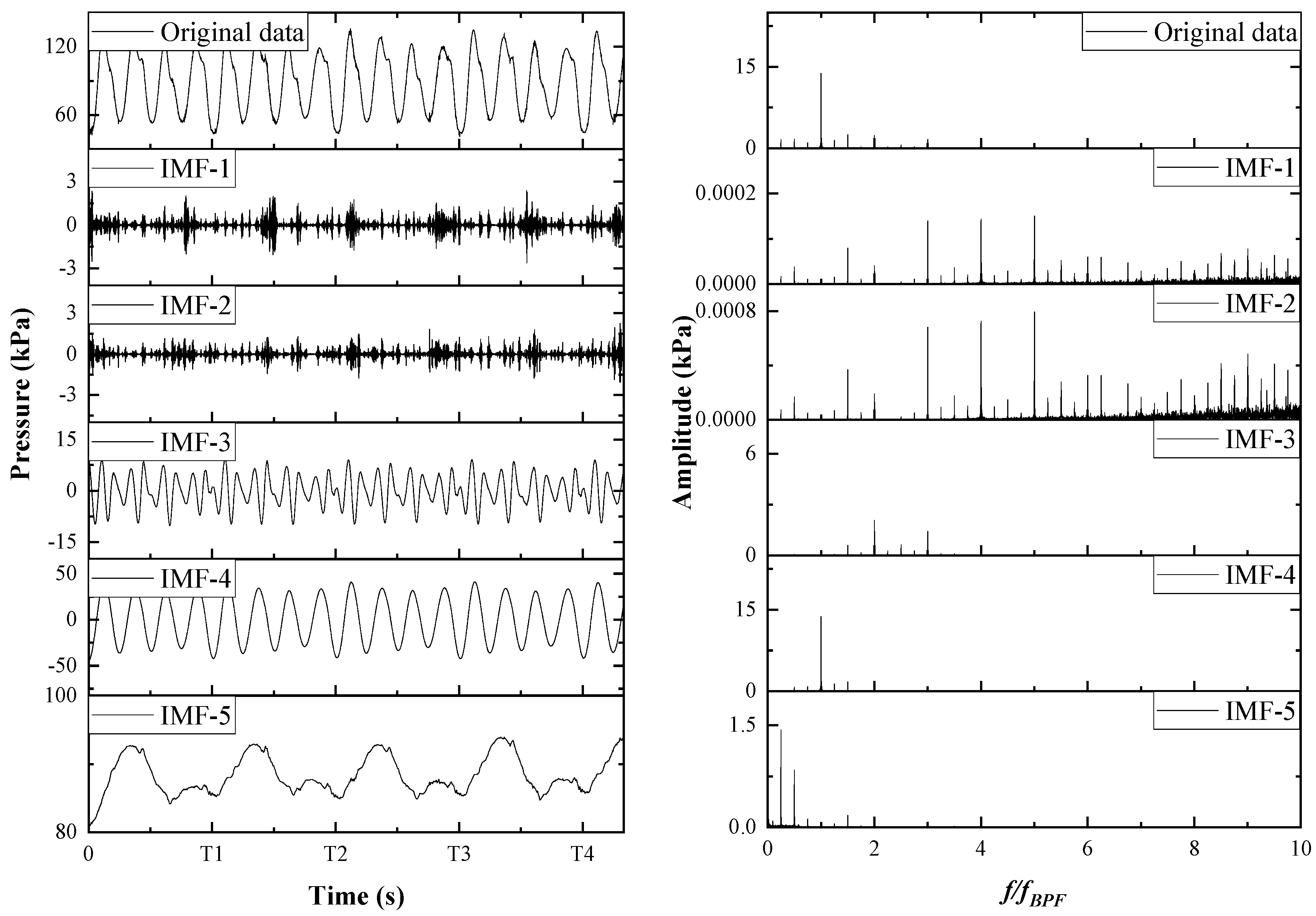
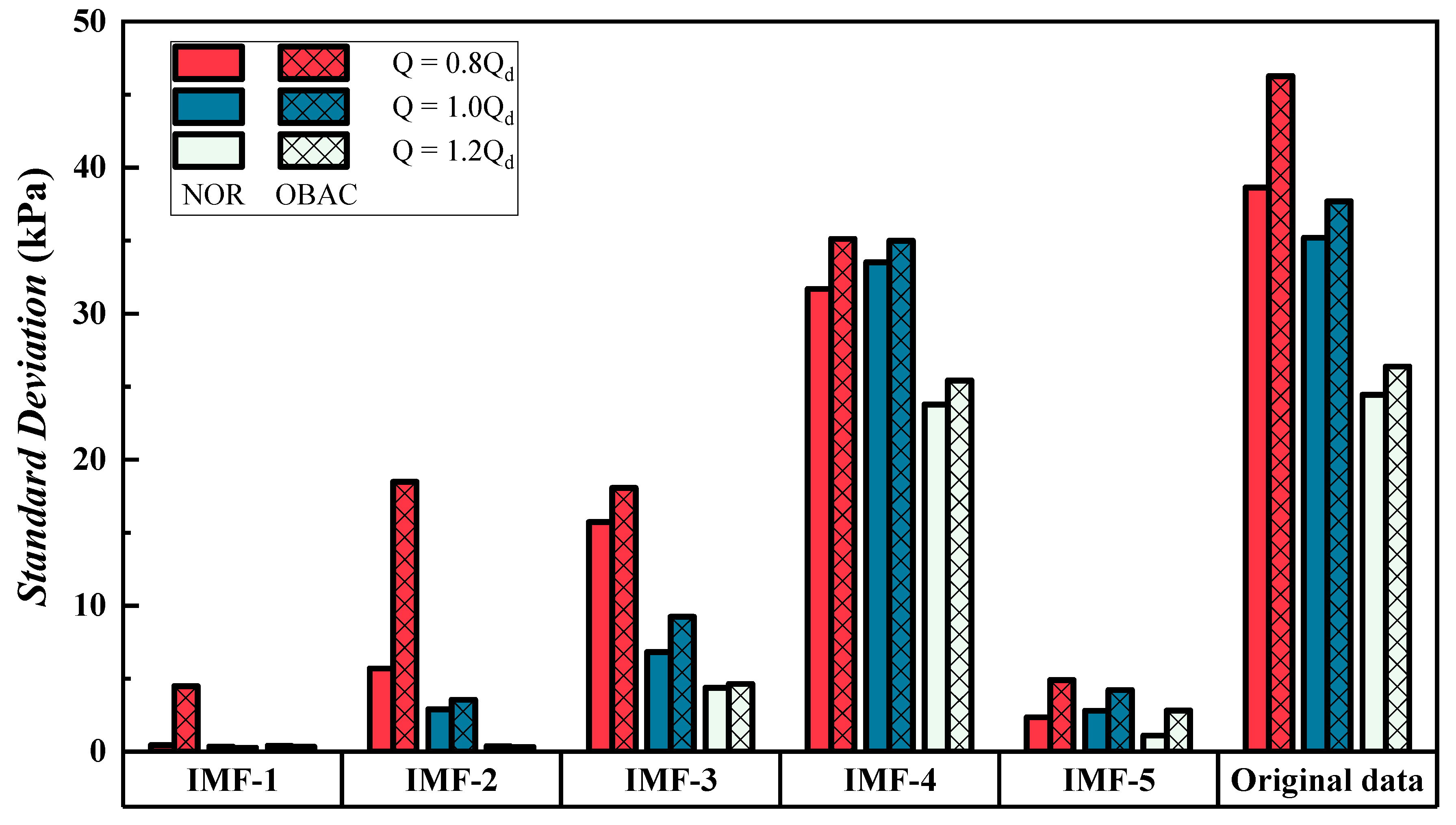
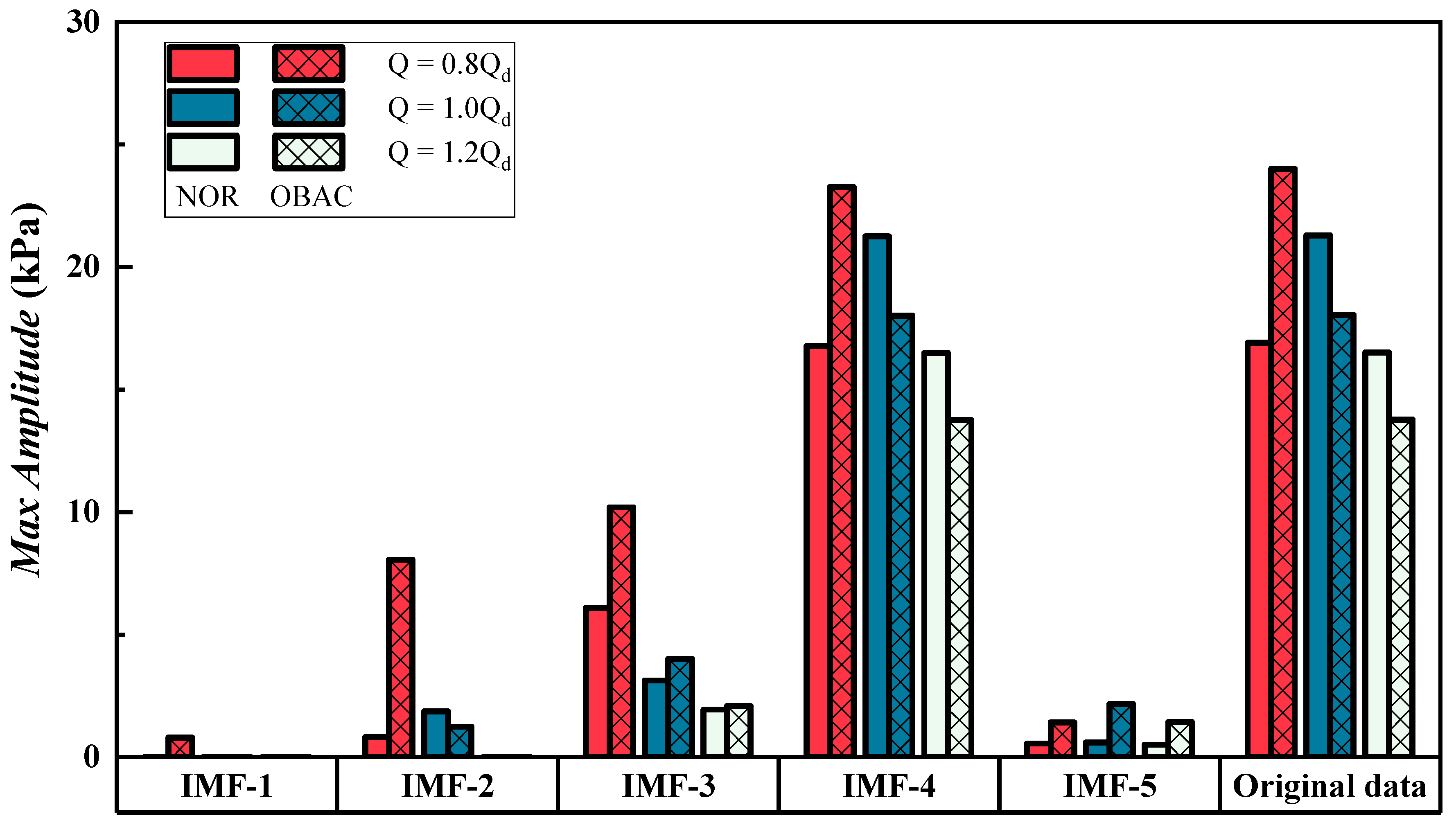
3.3. Pressure Pulsation after VMD Decomposition

The VMD method is capable of decomposing a complex signal into multiple modal components with different central frequencies. It can break down a complex signal into several harmonic signals and possesses characteristics such as adaptivity and robustness. Figure 11, Figure 12, Figure 13, Figure 14, Figure 15 and Figure 16 show the pressure pulsation signals and decomposition results under different working conditions and blade states, with the original data decomposed into five Intrinsic Mode Functions (IMFs). The left side of the figures displays the time-domain diagrams, with the horizontal axis representing the blade rotation cycle, mainly showing results for four cycles, and the vertical axis representing pressure. The right side of the figures shows the corresponding frequency-domain analysis results, with the horizontal axis representing the ratio of the transformed frequency to the blade-passing frequency (BPF). For ease of comparison, the vertical axis range is set to be the same for the same working condition.

Figure 10, Figure 11, Figure 12, Figure 13, Figure 14 and Figure 15 display the pressure pulsation signals and their decomposition results under different operating conditions and blade states. The original data are decomposed into five Intrinsic Mode Functions (IMFs). The left side of the figures shows the time-domain diagrams, with the horizontal axis representing the blade rotation cycle, mainly displaying results for four cycles, and the vertical axis representing pressure. The right side of the figures presents the corresponding frequency-domain analysis results, with the horizontal axis representing the ratio of the transformed frequency to the blade-passing frequency (BPF). To facilitate comparison, the vertical axis range is set to be the same for the results under the same operating condition.

Under the 0.8 Qd NOR blade condition, the frequencies of the components are distributed from high to low. The main frequency of the original data, IMF-1, and IMF-2 are above 4f/f_BPF, all of which are high-frequency components of the signal with very small amplitudes and can be essentially neglected. IMF-3 mainly decomposes the signal with obvious secondary peaks in the original signal, with frequencies mainly at 2f/f_BPF and 3f/f_BPF. IMF-4 decomposes the main frequency component of the original signal, with the largest amplitude and the greatest proportion. IMF-5 is dominated by frequencies below f/f_BPF. Comparing the NOR and OBAC conditions reveals that the main frequencies of the original signal at 0.8 Qd are primarily 1f/f_BPF, 2f/f_BPF, and 3f/f_BPF, with the OBAC condition having a higher main frequency. Under the OBAC condition, more high-frequency components are decomposed, and IMF-2, IMF-3, and IMF-5 all exhibit changes with the cycle.

At 1.0 Qd, the signal is much more stable than at 0.8 Qd, with the main frequency f/f_BPF amplitude significantly increased. Under the NOR condition, other harmonic components are noticeably reduced, with IMF-1 having a very small amplitude. IMF-2 to IMF-5, after decomposition, show signals that are relatively stable, with no obvious abnormal values appearing. Under the OBAC condition, the original data and the first four decompositions are similar to the results of the original data, and the waveforms after decomposition are also similar, indicating that even if one blade changes under the design condition, the pressure pulsation inside the pump still performs well. IMF-5, however, shows a significant difference between the two conditions, with OBAC producing a large peak value in each cycle, while the NOR condition is much more stable. The frequency shows that the main frequency decomposed by IMF-5 is 0.25f/f_BPF, which is the fluctuation signal produced by one blade, also indicating that one blade has experienced an anomaly.

Under the 1.2 Qd operating condition, the pressure pulsation waveform is simpler. Regardless of whether it is the NOR or OBAC condition, the main frequency of the original data is primarily f/f_BPF, with other harmonic signals being much smaller. After decomposition, the frequency-domain amplitudes of IMF-1 and IMF-2 become very small, with the main components concentrated in the low-frequency components. Similar to the 1.0 Qd condition, the signals of IMF-3 and IMF-4 are very similar after decomposition for both blade conditions, while IMF-5 is significantly different. Under the OBAC condition, a distinct peak appears in the time domain of IMF-5, and the frequency-domain signal is primarily 0.25 f/f_BPF, leading to the same conclusion as with the 1.0 Qd condition.

Figure 17 illustrates the standard deviation distribution of the original pressure pulsation data and the decomposed components. The magnitude of the standard deviation can measure the strength of the pulsation, which in this context is used to gauge the intensity of the signal in the decomposed components and under various operating conditions. Generally, IMF-4 has the greatest intensity, followed by IMF-3, with IMF-1 being the weakest. The pressure pulsation intensity at 0.8 Qd is the highest, followed by 1.0 Qd, and 1.2 Qd has the lowest. Under different blade conditions, the intensity is always greater in the OBAC condition than in the NOR condition, indicating that when the blade angle changes, it increases the overall pressure pulsation intensity within the pump.

Figure 18 shows the distribution of the main frequency amplitude of the original pressure pulsation data and the decomposed components. Overall, IMF-4 has the largest amplitude, followed by IMF-3, with IMF-1 being the weakest. Under the OBAC condition at 0.8 Qd, the main frequency amplitude is the highest, followed by 1.0 Qd, and 1.2 Qd has the lowest. However, under the NOR condition, the main frequency amplitude is mostly the highest at 1.0 Qd, and the lowest at 1.2 Qd. When comparing different blade conditions, at the 0.8 Qd operating condition, the OBAC main frequency amplitude is greater than that of the NOR condition; under other conditions, it is the NOR condition that has a greater amplitude. This indicates that when one blade angle changes, it reduces the main frequency amplitude and increases the components of the harmonic and sub-harmonic frequencies, and when in a low-flow condition, due to the more complex pulsation situation, a change in one blade angle can increase the amplitude of all components, intensifying the complexity of the flow.

4. Conclusions

We have analyzed the performance and pressure pulsation characteristics of an axial flow pump under two different blade conditions. By directly comparing the time domain, extracting the changes in peak-to-peak values of the pressure pulsation, and comparing the results after VMD decomposition, we have identified different methods for diagnosing blade characteristics and drawn the following conclusions:

(1)

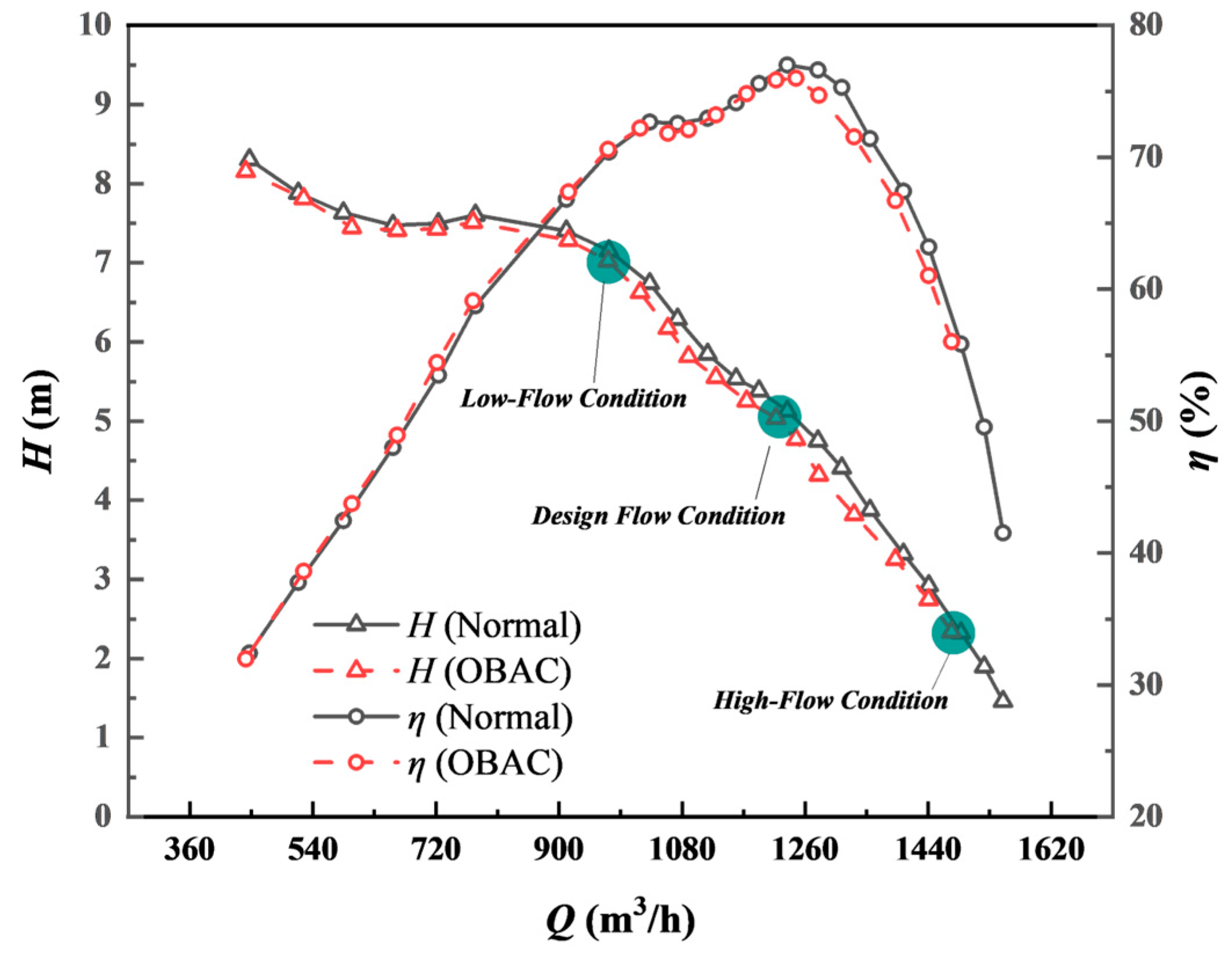
When one blade of an axial flow pump changes, it causes both the flow and head to decrease, with the head dropping by up to approximately 9.4% and the efficiency by up to about 3.5%. The effect on the head due to a change in the characteristics of one blade is more pronounced.

(2)

Even with the knowledge that one blade condition has changed, it is difficult to directly determine the change in blade condition from the time-domain results of the pressure pulsation. Extracting changes in peak-to-peak values can reveal significant variations at low- and design-flow rates, which interfere with the changes caused by blade alterations. At high-flow conditions, the pressure pulsation is simpler and more stable, allowing for the diagnosis of changes in blade angles through peak-to-peak values.

(3)

Decomposing the pressure pulsation using the VMD method yields different Intrinsic Mode Functions (IMFs). By examining the changes in low-frequency pulsations, it is possible to better diagnose changes in blade conditions, and the results can effectively exclude the influence of different flow conditions, making it a preferable diagnostic method.

References

1. Wang, L.; Tang, F.; Liu, H.; Zhang, X.; Sun, Z.; Wang, F. Investigation of Cavitation and Flow Characteristics of Tip Clearance of Bidirectional Axial Flow Pump with Different Clearances. Ocean Eng. 2023, 288, 115960. [Google Scholar] [CrossRef]
2. Wang, L.; Tang, F.; Chen, Y.; Liu, H. Evolution Characteristics of Suction-Side-Perpendicular Cavitating Vortex in Axial Flow Pump under Low Flow Condition. J. Mar. Sci. Eng. 2021, 9, 1058. [Google Scholar] [CrossRef]
3. Banaszek, A.; Petrović, R. Calculations of the Unloading Operation in Liquid Cargo Service with High Density on Modern Product and Chemical Tankers Equipped with Hydraulic Submerged Cargo Pumps. Stroj. Vestn. J. Mech. Eng. 2010, 56, 186–194. [Google Scholar]
4. Büker, J.; Laß, A.; Romig, S.; Werner, P.; Wurm, F.-H. On the effect of an ANC system towards the transient pressure fluctuations caused by smart-grid controlled centrifugal pumps. J. Renew. Sustain. Energy 2017, 9, 064502. [Google Scholar] [CrossRef]
5. Kan, K.; Xu, Z.; Chen, H.; Xu, H.; Zheng, Y.; Zhou, D.; Muhirwa, A.; Maxime, B. Energy Loss Mechanisms of Transition from Pump Mode to Turbine Mode of an Axial-Flow Pump under Bidirectional Conditions. Energy 2022, 257, 124630. [Google Scholar] [CrossRef]
6. Shi, L.; Yuan, Y.; Jiao, H.; Tang, F.; Cheng, L.; Yang, F.; Jin, Y.; Zhu, J. Numerical Investigation and Experiment on Pressure Pulsation Characteristics in a Full Tubular Pump. Renew. Energy 2021, 163, 987–1000. [Google Scholar] [CrossRef]
7. Spence, R.; Amaral-Teixeira, J. Investigation into Pressure Pulsations in a Centrifugal Pump Using Numerical Methods Supported by Industrial Tests. Comput. Fluids 2008, 37, 690–704. [Google Scholar] [CrossRef]
8. Fu, X.; Li, D.; Lv, J.; Yang, B.; Wang, H.; Wei, X. High-Amplitude Pressure Pulsations Induced by Complex Inter-Blade Flow during Load Rejection of Ultrahigh-Head Prototype Pump Turbines. Phys. Fluids 2024, 36, 034115. [Google Scholar] [CrossRef]
9. Lu, J.; Liu, J.; Qian, L.; Liu, X.; Yuan, S.; Zhu, B.; Dai, Y. Investigation of Pressure Pulsation Induced by Quasi-Steady Cavitation in a Centrifugal Pump. Phys. Fluids 2023, 35, 025119. [Google Scholar] [CrossRef]
10. Song, X.; Liu, C. Experimental Investigation of Floor-Attached Vortex Effects on the Pressure Pulsation at the Bottom of the Axial Flow Pump Sump. Renew. Energy 2020, 145, 2327–2336. [Google Scholar] [CrossRef]
11. Cao, W.; Liu, Y.; Dong, J.; Niu, Z.; Shi, Y. Research on Pressure Pulsation Characteristics of Gerotor Pump for Active Vibration Damping System. IEEE Access 2019, 7, 116567–116577. [Google Scholar] [CrossRef]
12. Zhang, N.; Li, D.; Gao, B.; Ni, D.; Li, Z. Unsteady Pressure Pulsations in Pumps—A Review. Energies 2023, 16, 150. [Google Scholar] [CrossRef]
13. Zhang, F.; Xiao, R.; Zhu, D.; Liu, W.; Tao, R. Pressure Pulsation Reduction in the Draft Tube of Pump Turbine in Turbine Mode Based on Optimization Design of Runner Blade Trailing Edge Profile. J. Energy Storage 2023, 59, 106541. [Google Scholar] [CrossRef]
14. Wang, W.; Pei, J.; Yuan, S.; Yin, T. Experimental Investigation on Clocking Effect of Vaned Diffuser on Performance Characteristics and Pressure Pulsations in a Centrifugal Pump. Exp. Therm. Fluid Sci. 2018, 90, 286–298. [Google Scholar] [CrossRef]
15. Binama, M.; Su, W.-T.; Cai, W.-H.; Li, X.-B.; Muhirwa, A.; Li, B.; Bisengimana, E. Blade Trailing Edge Position Influencing Pump as Turbine (PAT) Pressure Field under Part-Load Conditions. Renew. Energy 2019, 136, 33–47. [Google Scholar] [CrossRef]
16. Trivedi, C.; Gogstad, P.J.; Dahlhaug, O.G. Investigation of the unsteady pressure pulsations in the pro-totype Francis turbines during load variation and startup. J. Renew. Sustain. Energy 2017, 9, 064502. [Google Scholar] [CrossRef]
17. Sonawat, A.; Kim, S.; Ma, S.-B.; Kim, S.-J.; Lee, J.B.; Yu, M.S.; Kim, J.-H. Investigation of Unsteady Pressure Fluctuations and Methods for Its Suppression for a Double Suction Centrifugal Pump. Energy 2022, 252, 124020. [Google Scholar] [CrossRef]
18. Zhang, S.; Chen, H.; Ma, Z.; Wang, D.; Ding, K. Unsteady Flow and Pressure Pulsation Characteristics in Centrifugal Pump Based on Dynamic Mode Decomposition Method. Phys. Fluids 2022, 34, 112014. [Google Scholar] [CrossRef]
19. Fang, M.; Zhang, F.; Cao, Z.; Tao, R.; Xiao, W.; Zhu, D.; Gui, Z.; Xiao, R. Prediction Accuracy Improvement of Pressure Pulsation Signals of Reversible Pump-Turbine: A LSTM and VMD-Based Optimization Approach. Energy Sci. Eng. 2024, 12, 102–116. [Google Scholar] [CrossRef]
20. Ren, Y.; Zhang, L.; Chen, J.; Liu, J.; Liu, P.; Qiao, R.; Yao, X.; Hou, S.; Li, X.; Cao, C.; et al. Noise Reduction Study of Pressure Pulsation in Pumped Storage Units Based on Sparrow Optimization VMD Combined with SVD. Energies 2022, 15, 2073. [Google Scholar] [CrossRef]
21. Zhou, T.; Yu, X.; Zhang, J.; Xu, H. Analysis of Transient Pressure of Pump-Turbine during Load Rejection Based on a Multi-Step Extraction Method. Energy 2024, 292, 130578. [Google Scholar] [CrossRef]
22. Zhang, F.; Fang, M.; Tao, R.; Liu, W.; Gui, Z.; Xiao, R. Investigation of Energy Loss Patterns and Pressure Fluctuation Spectrum for Pump-Turbine in the Reverse Pump Mode. J. Energy Storage 2023, 72, 108275. [Google Scholar] [CrossRef]
Figure 1. High-precision hydraulic machinery test bench.
Jmse 12 01586 g001
Figure 2. Schematic diagram of the test pump system and its dimensions (unit: mm).
Jmse 12 01586 g002
Figure 3. Installation position of pressure pulsation measurement.
Jmse 12 01586 g003
Figure 4. Relative position of pressure pulsation measurement points and blades.
Jmse 12 01586 g004
Figure 5. External characteristics of axial flow pump under different blade conditions.
Jmse 12 01586 g005
Figure 6. Time-domain variation in pressure fluctuations under different blade conditions at 0.8 Qd. The red line indicates the trend of the trough. Red wireframes and circles mark abnormal changes in pressure pulsation.
Jmse 12 01586 g006
Figure 7. Time-domain variation in pressure fluctuations under different blade conditions at 1.0 Qd. The red line indicates the trend of the trough. Red wireframes and circles mark abnormal changes in pressure pulsation.
Jmse 12 01586 g007
Figure 8. Time-domain variation in pressure fluctuations under different blade conditions at 1.2 Qd. The red line indicates the trend of the trough. Red circles mark abnormal changes in pressure pulsation.
Jmse 12 01586 g008
Figure 9. Signal smoothing and peak and trough extraction.
Jmse 12 01586 g009
Figure 10. Variation of peak-to-peak values.
Jmse 12 01586 g010
Figure 11. Time- and frequency-domain diagrams of pressure pulsation and its decomposition results in the case of 0.8 Qd-NOR.
Jmse 12 01586 g011
Figure 12. Time- and frequency-domain diagrams of pressure pulsation and its decomposition results in the case of 0.8 Qd-OBAC.
Jmse 12 01586 g012
Figure 13. Time- and frequency-domain diagrams of pressure pulsation and its decomposition results in the case of 1.0 Qd-NOR.
Jmse 12 01586 g013
Figure 14. Time- and frequency-domain diagrams of pressure pulsation and its decomposition results in the case of 1.0 Qd-OBAC.
Jmse 12 01586 g014
Figure 15. Time- and frequency-domain diagrams of pressure pulsation and its decomposition results in the case of 1.2 Qd-NOR.
Jmse 12 01586 g015
Figure 16. Time- and frequency-domain diagrams of pressure pulsation and its decomposition results in the case of 1.2 Qd-OBAC.
Jmse 12 01586 g016
Figure 17. Standard deviation distribution of raw data and decomposed data of pressure pulsation.
Jmse 12 01586 g017
Figure 18. Maximum amplitude distribution in frequency domain of raw data and decomposed data of pressure pulsation.
Jmse 12 01586 g018