A Bio-Inspired Sliding Mode Method for Autonomous Cooperative Formation Control of Underactuated USVs with Ocean Environment Disturbances

Abstract

In this paper, a bio-inspired sliding mode control (bio-SMC) and minimal learning parameter (MLP) are proposed to achieve the cooperative formation control of underactuated unmanned surface vehicles (USVs) with external environmental disturbances and model uncertainties. Firstly, the desired trajectory of the follower USV is generated by the leader USV’s position information based on the leader–follower framework, and the problem of cooperative formation control is transformed into a trajectory tracking error stabilization problem. Besides, the USV position errors are stabilized by a backstepping approach, then the virtual longitudinal and virtual lateral velocities can be designed. To alleviate the system oscillation and reduce the computational complexity of the controller, a sliding mode control with a bio-inspired model is designed to avoid the problem of differential explosion caused by repeated derivation. A radial basis function neural network (RBFNN) is adopted for estimating and compensating for the environmental disturbances and model uncertainties, where the MLP algorithm is utilized to substitute for online weight learning in a single-parameter form. Finally, the proposed method is proved to be uniformly and ultimately bounded through the Lyapunov stability theory, and the validity of the method is also verified by simulation experiments.

1. Introduction

Recently, due to significant advancements in marine science and technology, such as marine resource exploration, maritime casualty and ocean mapping [1,2,3,4], the intelligent control of unmanned surface vehicles (USVs) has become a hot topic. As small intelligent unmanned maritime carrier platforms, USVs can replace humans to perform various complex tasks, particularly in harsh marine environments [5,6]. However, with the increasing complexity and diversity of maritime operations, a single USV often struggles to efficiently accomplish these tasks [7,8]. In response to this challenge, the cooperative formation of multiple USVs has gained widespread attention [9,10]. One significant problem concerned with multiple USVs is formation tracking control, which requires the USVs to keep a prescribed formation while USVs are navigating along a given desired trajectory [11,12]. A number of related research works on the autonomous cooperative formation control of USVs have been carried out, and many valuable research results have been published.

A novel terminal sliding surface control (TSMC) was designed by [13] to solve the cooperative formation control problem of unmanned surface vehicle-remotely operated vehicles (USV-ROVs) subject to uncertainties under deceptive attacks. The USV’s dynamic model was established by [14] for the leader–follower formation in polar coordinates, where a sliding mode control is employed to design the controller. Based on the leader–follower framework, USV formation control was designed by utilizing the model predictive control (MPC) algorithm [15]. Combined with the leader–follower formation strategy, a deep reinforcement learning (DRL) algorithm was introduced in [16], where the follower USVs can self-adjust even through deviating from the formation. A hierarchical sliding mode control strategy was designed to solve the formation control problem of USVs based on the sampling communication by [17], where a sign function was developed for the sliding mode control. In [18], an adaptive sliding mode control was used to reduce system oscillations, and the hyperbolic tangent function was employed to enhance the robustness of the control system. A distributed control law was designed by [19] based on a novel sliding surface in which the constructed sliding surface is capable of being reached in a finite time.

On account of the time-varying external disturbances and mode uncertainties, two novel distributed coordinated finite time-tracking controllers were proposed based on the sliding mode control method in [20], and the radial basis function neural networks (RBFNNs) combined with the minimal learning parameter (MLP) was applied in [21]. Combined with a lateral velocity tracking differentiator (LVTD), a novel dynamic surface sliding mode control (DSSMC) method was designed by [22] for the cooperative formation control of underactuated USVs with complex disturbances. The OAST-SMC with backstepping method was employed to solve the external disturbances and enhance the precision of formation control in [23]. An accurate disturbance observer (ADO) and a novel fixed-time fast terminal sliding mode (FTFTSM) were designed for parametric uncertainties and complex disturbances [24]. To investigate the formation tracking control problem of networked USVs under a directed graph, a prescribed-time distributed cooperative formation tracking control scheme was provided by [25], where the prescribed-time sliding surface was designed based on the state observer.

Through the analysis of the above existing research results, it should be pointed out that, in studies [14,15,16], the problem of cooperative formation control was addressed based on the leader–follower framework. The cooperative formation control algorithms of USVs were designed for fully actuated USVs in [19,24,25]; however, due to factors such as system dynamic characteristics and physical constraints in the actual engineering practice, the control system may become underactuated. Meanwhile, autonomous cooperative formation control problems were solved by using the sliding mode method in [13,17,18,20,21], but the problem of differential explosion was not discussed in these paper. This problem is caused by repeated derivation during the sliding mode design process and may increase the computational complexity of the controller and the system oscillation. Besides, although the complex ocean environment disturbances were addressed in [22,23,25], the problem of model uncertainties was not considered.

Motivated by the above analysis, to address the control problem of USV formation with ocean environment disturbances and model uncertainties, a bio-inspired sliding mode control (bio-SMC) method is designed in this paper. Based on the leader–follower framework, the problem of cooperative formation control is transformed into a trajectory tracking error stabilization problem for each USV, and then the virtual control laws of the longitudinal and lateral velocities are designed by using a backstepping method to stabilize the position error. A sliding mode control with a bio-inspired model is designed to alleviate the system oscillation and reduce the computational complexity of the controller, and then the problem of differential explosion caused by repeated derivation could be avoided. Besides, a radial basis function neural network (RBFNN) with the MLP algorithm is adopted for estimating and compensating for the environmental disturbances and model uncertainties. Compared with the existing research results, the main contributions of this paper can be summarized as follows: (1) Based on the leader–follower framework, the virtual longitudinal and lateral velocities are designed by using the backstepping method, and then the controller design can become more convenient. (2) The second-order sliding surface with an integral is constructed for reducing steady-state error, and a hyperbolic tangent function is employed in place of the sign function to reduce system oscillations. (3) A bio-inspired model is designed to avoid the problem of differential explosion caused by repeated derivation, and then the virtual velocities can be smoothed. (4) A radial basis function neural network (RBFNN) with the minimal learning parameter (MLP) algorithm is adopted for approximating the environmental disturbances and model uncertainties.

This paper is organized as follows: the mathematical model of USV and error model of USV formation are described in Section 2. In Section 3, the control law including the surge force and the yaw moment are described. The stability of the controller is proved in Section 4. The simulation experiments are presented to verify the accuracy and effectiveness of the proposed method in Section 5. Finally, the conclusion is given in Section 6.

2. Problem Description

A coordinated formation control algorithm of USVs is designed in this paper, through which the formation trajectory tracking issue can be addressed effectively. The formation trajectory tracking problem can be described as shown in Figure 1.

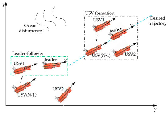
Figure 1. Formation trajectory tracking diagram.

The formation trajectory tracking problem can be considered as how the USV formation should navigate along the desired trajectory under the influence of ocean disturbances, where each USV is required to maintain the predefined formation relative to other USVs. To achieve the problem mentioned above, the model of USVs and the tracking error model of USV formation are built, as shown in Section 2.1 and Section 2.2.

2.1. Mathematical Model of USV

As shown in Figure 1, assume that there exist $N$ USVs in formation, which includes one leader USV and $N-1$ follower USVs. According to the literature [26], the mathematical model of the $i^{th}(i=1,2,\cdots ,N)$ USV under the influence of ocean disturbances and model uncertainties can be expressed as follows:

$$\left\{\begin{array}{l}{\dot{\eta }}_i=R({\phi }_i)v_i\\ M_i{\dot{v}}_i+C_i(v_i)v_i+D_i(v_i)v_i={\tau }_i+d_i+\Delta f_i\end{array}\right.$$

(1)

where ${\eta }_i={[x_i,y_i,{\phi }_i]}^T$ is the position and heading angle vector of the $i^{th}$ USV, in which $x_i$ is the longitudinal position, $y_i$ is the lateral position and ${\phi }_i$ is the heading angle. $v_i={[u_i,v_i,r_i]}^T$ represents the velocity vector of the $i^{th}$ USV, in which $u_i$, $v_i$ and $r_i$ are the longitudinal velocity, lateral velocity and heading angle speed. ${\tau }_{ci}={[{\tau }_{ui},0,{\tau }_{ri}]}^T$ is the control input vector of the $i^{th}$ USV. $d_i={[d_{ui},d_{vi},d_{ri}]}^T$ represents the external disturbances vector of the $i^{th}$ USV. $\Delta f_i={[\Delta f_{u_i},\Delta f_{v_i},\Delta f_{r_i}]}^T$ denotes the model uncertainties of the $i^{th}$ USV. $M_i=diag(m_{1i},m_{2i},m_{3i})$ is the inertia matrix including added mass of the $i^{th}$ USV. ${\mathit{D}}_i(v_i)=diag(d_{1i},d_{2i},d_{3i})$ represents the hydrodynamic damping coefficient matrix of the $i^{th}$ USV. $R({\phi }_i)$,${\mathit{C}}_i(v_i)$ are the rotation matrix and the Coriolis-centripetal matrix of the $i^{th}$ USV, specifically defined as follows:

$$R({\phi }_i)=\left[\begin{array}{ccc}\cos {\phi }_i& -\sin {\phi }_i& 0\\ \sin {\phi }_i& \cos {\phi }_i& 0\\ 0& 0& 1\end{array}\right],C(v_i)=\left[\begin{array}{ccc}0& 0& -m_{2i}{v}_i\\ 0& 0& m_{1i}{u}_i\\ m_{2i}{v}_i& m_{1i}{u}_i& 0\end{array}\right]$$

According to Equation (1), the model of the $i^{th}$ USV with three degrees of mathematical freedom can be expanded as follows:

$$\left\{\begin{array}{l}{\dot{x}}_i=u_i\cos {\phi }_i-v_i\sin {\phi }_i\\ {\dot{y}}_i=u_i\sin {\phi }_i+v_i\cos {\phi }_i\\ {\dot{\phi }}_i=r_i\\ {\dot{u}}_i=f_{u_i}(u_i,v_i,r_i)+{\tau }_{ui}/m_{1i}\\ {\dot{v}}_i=f_{v_i}(u_i,v_i,r_i)\\ {\dot{r}}_i=f_{r_i}(u_i,v_i,r_i)+{\tau }_{ri}/m_{3i}\end{array}\right.$$

(2)

where the specific expressions of the $f_{u_i}(u_i,v_i,r_i),f_{v_i}(u_i,v_i,r_i),f_{r_i}(u_i,v_i,r_i)$ are as follows:

$$\left\{\begin{array}{l}{f}_{u_i}(u_i,v_i,r_i)=\left(m_{2i}/m_{1i}\right)v_i{r}_i-\left(d_{1i}/m_{1i}\right)u_i+d_{ui}/m_{1i}+\Delta f_{u_i}\\ f_{v_i}(u_i,v_i,r_i)=-\left(m_{1i}/m_{2i}\right)u_i{r}_i-\left(d_{2i}/m_{2i}\right)v_i+d_{vj}/m_{2i}+\Delta f_{v_i}\\ f_{r_i}(u_i,v_i,r_i)=\left(\left(m_{1i}-m_{2i}\right)/m_{3i}\right)u_i{v}_i-\left(d_{3i}/m_{3i}\right)r_i+d_{ri}/m_{3i}+\Delta f_{r_i}\end{array}\right.$$

(3)

2.2. Error Model of USV Formation

The leader–follower framework proposed in Figure 1 is designed to maintain a predefined formation while USVs are navigating, as specifically described in Figure 2 below:

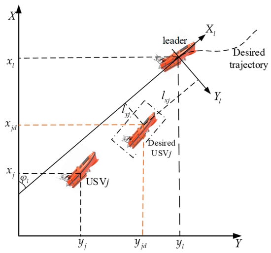
Figure 2. Leader–follower framework.

As shown in Figure 2, the $j^{\mathrm{th}}\left(j=1,2,\dots ,N-1\right)$ USV serves as the follower USV for the leader USV. $Y_l={[x_l,y_l]}^T$ is the position vector of the leader USV. $Y_j={[x_j,y_j]}^T$ is the position vector of the $j^{\mathrm{th}}$ follower USV. ${\phi }_l$ is the heading angle of the leader USV; $L_j={[l_{xj},l_{yj}]}^T$ is the formation position vector from the $j^{\mathrm{th}}$ follower USV to the leader USV, where $l_{xj}$ is the desired relative longitudinal position in the coordinate system of the leader USV and $l_{yj}$ is the desired relative lateral position in the coordinate system of the leader USV. $Y_{jd}={[x_{jd},y_{jd}]}^T$ is the desired position vector of the $j^{\mathrm{th}}$ follower USV, where $x_{jd}$ is the desired longitudinal position of the $j^{\mathrm{th}}$ follower USV and $y_{jd}$ is the desired lateral position of the $j^{\mathrm{th}}$ follower USV. The desired position of the $j^{\mathrm{th}}$ follower USV can be expressed as follows:

$$Y_{jd}=Y_l+J({\phi }_l)\cdot L_j$$

(4)

where $J({\phi }_l)=\left[\begin{array}{cc}\cos ({\phi }_l)& -\sin ({\phi }_l)\\ \sin ({\phi }_l)& \cos ({\phi }_l)\end{array}\right]$ is the standard rotation matrix.

Based on the above analysis, the trajectory tracking problem of the $j^{\mathrm{th}}$ follower USV could be transformed to design a suitable control ${\tau }_i$ that ensures tracking error $Y_{je}=Y_j-Y_{jd}$ approaches zero.

3. Controller Design

As shown in Figure 1, to enable USVs to track a desired trajectory in a specified formation, it is crucial to design an appropriate control algorithm. The flowchart of cooperative formation control of USVs is designed as shown in Figure 3.

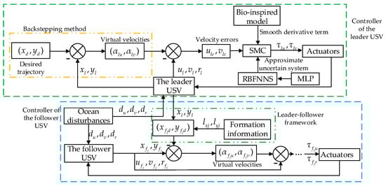
Figure 3. Flowchart of cooperative formation control for underactuated USVs.

As seen in Figure 3, the cooperative formation control process of USVs can be divided into two main parts: the controller of the lead USV would be designed by a backstepping method and the bio-inspired sliding model method. Then, the actual trajectory of the leader USV and formation information are used to generate the desired trajectories for each follower USV, and the controllers of the follower USVs would be designed the same as for the leader USV, which includes the design of the virtual velocity control law in Section 3.1, the design of the surge force controller in Section 3.2 and the design of the yaw moment controller in Section 3.3.

3.1. Design of Virtual Velocities

As seen in Figure 3, it is crucial for the controller to design virtual velocities based on the position errors. The position errors of the $j^{\mathrm{th}}$ follower USV could be proposed as follows:

$$\left[\begin{array}{c}{x}_{f_{j}e}\\ y_{f_{j}e}\end{array}\right]=\left[\begin{array}{c}{x}_{f_j}-x_{f_{j}d}\\ y_{f_j}-y_{f_{j}d}\end{array}\right]$$

(5)

where $x_{f_j},y_{f_j}$ are the actual longitudinal position and lateral position of the $j^{\mathrm{th}}$ follower USV and $x_{f_{j}d},y_{f_{j}d}$ are the desired longitudinal position and lateral position of the $j^{\mathrm{th}}$ follower USV. $x_{f_{j}e},y_{f_{j}e}$ are longitudinal position error and lateral position error of the $j^{\mathrm{th}}$ follower USV.

Combining this with Equation (2), the derivation of Equation (5) could be written as follows:

$$\left[\begin{array}{l}{\dot{x}}_{f_{j}e}\\ {\dot{y}}_{f_{j}e}\end{array}\right]=\left[\begin{array}{cc}\cos ({\phi }_{f_j})& -\sin ({\phi }_{f_j})\\ \sin ({\phi }_{f_j})& \cos ({\phi }_{f_j})\end{array}\right]\left[\begin{array}{l}{u}_{f_j}\\ v_{f_j}\end{array}\right]-\left[\begin{array}{l}{\dot{x}}_{f_{j}d}\\ {\dot{y}}_{f_{j}d}\end{array}\right]$$

(6)

where $u_{f_j},v_{f_j}$ are the actual longitudinal velocity and lateral velocity of the $j^{\mathrm{th}}$ follower USV. ${\phi }_{f_j}$ is the actual heading angle of the $j^{\mathrm{th}}$ follower USV.

To stabilize the position errors of the $j^{\mathrm{th}}$ follower, the Lyapunov function could be designed as follows:

$$V_{1f_i}=x_{f_{i}e}^2/2+y_{f_{i}e}^2/2$$

(7)

Combining this with Equations (2) and (6), the derivation of Equation (7) can be obtained as follows:

$$\begin{array}{cc}{\dot{V}}_{1f_i}& ={\displaystyle \frac{\partial V_{1f_i}}{\partial x_{f_{i}e}}}{\displaystyle \frac{\partial x_e}{\partial t}}+{\displaystyle \frac{\partial V_{1f_i}}{\partial y_{f_{i}e}}}{\displaystyle \frac{\partial y_{f_{i}e}}{\partial t}}\hfill \\ & =x_{f_{i}e}{\dot{x}}_{f_{i}e}+y_{f_{i}e}{\dot{y}}_{f_{i}e}\hfill \\ & =x_{f_{i}e}(u_{f_j}\cos ({\phi }_{f_j})-v_{f_j}\sin ({\phi }_{f_j})-{\dot{x}}_{f_{j}d})+y_{f_{i}e}(u_{f_j}\sin ({\phi }_{f_j})+v_{f_j}\cos ({\phi }_{f_j})-{\dot{y}}_{f_{j}d})\hfill \end{array}$$

(8)

Generally, the values of virtual velocities ${\alpha }_{f_{j}u}$ and ${\alpha }_{f_{j}v}$ are related to the position errors, and based on the backstepping method, the virtual velocities ${\alpha }_{f_{j}u}$ and ${\alpha }_{f_{j}v}$ of the $j^{\mathrm{th}}$ follower USV could be designed as follows:

$$\left[\begin{array}{l}{\alpha }_{f_{j}u}\\ {\alpha }_{f_{j}v}\end{array}\right]=\left[\begin{array}{cc}\cos ({\phi }_{f_j})& \sin ({\phi }_{f_j})\\ -\sin ({\phi }_{f_j})& \cos ({\phi }_{f_j})\end{array}\right]\left[\begin{array}{l}{\dot{x}}_{f_{j}d}-k_{1f_j}{x}_{f_{j}e}/\sqrt{x_{f_{j}e}^2+y_{f_{j}e}^2+C_{f_j}}\\ {\dot{y}}_{f_{j}d}-k_{2f_j}{y}_{f_{j}e}/\sqrt{x_{f_{j}e}^2+y_{f_{j}e}^2+C_{f_j}}\end{array}\right]$$

(9)

where $k_{1f_j},k_{2f_j},C_{f_j}$ are positive numbers.

Based on the above analysis, the trajectory tracking problem of the $j^{\mathrm{th}}$ follower USV could be transformed to design a suitable control ${\tau }_j$ that ensures errors of the virtual velocities and actual velocities approach zero.

3.2. Design of the Surge Force

Utilizing the virtual longitudinal velocity ${\alpha }_{f_{j}u}$ designed in Section 3.1, the surge force of the $j^{\mathrm{th}}$ follower USV could be designed based on the bio-inspired sliding mode method. Define the longitudinal velocity error $u_{f_{j}e}$ as follows:

$$u_{f_{j}e}=u_{f_j}-{\alpha }_{f_{j}u}$$

(10)

To reduce the steady-state error, the integral sliding surface $s_{1f_j}$ with $u_{f_{j}e}$ could be designed as follows:

$$s_{1f_j}=u_{f_{j}e}+{\lambda }_{1f_j}{\displaystyle {\int }_0^t{u}_{f_{j}e}(s)ds}$$

(11)

where ${\lambda }_{1f_j}$ is a positive number.

Combining this with the Equation (2), the derivation of Equation (11) could be obtained as follows:

$$\begin{array}{cc}{\dot{s}}_{1f_j}& ={\dot{u}}_{f_j}-{\dot{\alpha }}_{f_{j}u}+{\lambda }_{1f_j}{u}_{f_{j}e}\hfill \\ & =f_{f_{j}u}(u_{f_j},v_{f_j},r_{f_j})+{\tau }_{uj}/m_{1j}-{\dot{\alpha }}_{f_{j}u}+{\lambda }_{1f_j}{u}_{f_{j}e}\hfill \end{array}$$

(12)

In order to avoid differential explosion caused by repeated derivation and smooth the virtual velocity ${\alpha }_{f_{j}u}$, the bio-inspired model could be designed [27], where the virtual longitudinal velocity derivative ${\dot{\alpha }}_{f_{i}u}$ in Equation (12) is transformed into ${\dot{\beta }}_{f_{j}u}$, shown as follows:

$$\begin{array}{l}{\dot{\beta }}_{f_{j}u}=-B_{1f_j}{\beta }_{f_{j}u}+(C_{1f_j}-{\beta }_{f_{j}u})f({\alpha }_{f_{j}u})-(D_{1f_j}+{\beta }_{f_{j}u})g({\alpha }_{f_{j}u})\\ f({\alpha }_{f_{j}u})=\left\{\begin{array}{l}{\alpha }_{f_{j}u},{\alpha }_{f_{j}u}\ge 0\\ 0,{\alpha }_{f_{j}u}<0\end{array}\right.,g({\alpha }_{f_{j}u})=\left\{\begin{array}{l}0,{\alpha }_{f_{j}u}>0\\ -{\alpha }_{f_{j}u},{\alpha }_{f_{j}u}\le 0\end{array}\right.\end{array}$$

(13)

where ${\beta }_{f_{j}u}$ is the output of the bio-inspired model. $B_{1f_j}$ represents the model of the attenuation rate and is the positive constant. $C_{1f_j}$ and $D_{1f_j}$ denote the upper and lower bounds of the ${\beta }_{f_{i}u}$. $f({\alpha }_{f_{j}u})$ and $g({\alpha }_{f_{j}u})$ are linear threshold functions.

To prevent the system oscillation caused by using the sign function, Equation (14) could be designed with a hyperbolic tangent function, listed as follows:

$${\dot{s}}_{1f_j}=-{\epsilon }_{1f_j}\tanh (s_{1f_j})-{\sigma }_{1f_j}{s}_{1f_j}$$

(14)

where ${\epsilon }_{1f_j}$ and ${\sigma }_{1f_j}$ are positive numbers.

Combining this with the Equations (12)–(14), the surge force of the $j^{\mathrm{th}}$ follower USV could be obtained as follows:

$${\tau }_{f_{j}u}=m_{1j}[-f_{f_{j}u}(u_{f_j},v_{f_j},r_{f_j})+{\dot{\beta }}_{f_{j}u}-{\lambda }_{1f_j}{u}_{f_{j}e}-{\epsilon }_{1f_j}\tanh (s_{1f_j})-{\sigma }_{1f_j}{s}_{1f_j}]$$

(15)

3.3. Design of the Yaw Moment

Utilizing the virtual lateral velocity ${\alpha }_{f_{j}v}$ designed in Section 3.1, the yaw moment of the $j^{\mathrm{th}}$ follower USV could be designed based on the bio-inspired sliding mode method. Define the lateral velocity error $v_{f_{j}e}$ as follows:

$$v_{f_{j}e}=v_{f_j}-{\alpha }_{f_{j}v}$$

(16)

where $v_{f_j}$ is the actual lateral velocity of the $j^{\mathrm{th}}$ follower USV.

Due to the lack of a controller in the lateral direction for the underactuated USV, the second-order integral sliding surface with the lateral velocity error $v_{f_{j}e}$ could be designed as follows:

$$s_{2f_j}={\dot{v}}_{f_{j}e}+{\lambda }_{2f_j}{v}_{f_{j}e}+{\lambda }_{3_j}{\displaystyle {\int }_0^t{v}_{f_{j}e}(s)ds}$$

(17)

where ${\lambda }_{2f_j}$ and ${\lambda }_{3f_j}$ are positive numbers.

Combining this with the Equation (2), the derivation of Equation (17) could be obtained as follows:

$${\dot{s}}_{2f_j}={\ddot{v}}_{f_j}-{\ddot{\alpha }}_{f_{j}v}+{\lambda }_{2f_j}({\dot{v}}_{f_j}-{\dot{\alpha }}_{f_{j}v})+{\lambda }_{3_j}(v_{f_j}-{\alpha }_{f_{j}v})$$

(18)

To obtain ${\ddot{\alpha }}_{f_{j}v}$ in Equation (18), the derivation of Equation (9) is proposed as follows:

$$\begin{array}{cc}\left[\begin{array}{l}{\dot{\alpha }}_{f_{j}u}\\ {\dot{\alpha }}_{f_{j}v}\end{array}\right]& =r_{f_j}\left[\begin{array}{cc}-\sin ({\phi }_{f_j})& \cos ({\phi }_{f_j})\\ -\cos ({\phi }_{f_j})& -\sin ({\phi }_{f_j})\end{array}\right]\left[\begin{array}{l}{\dot{x}}_{f_{j}d}-k_{1f_j}{w}_{f_j}^{-1}{x}_{f_{j}e}\\ {\dot{y}}_{f_{j}d}-k_{2f_j}{w}_{f_j}^{-1}{y}_{f_{j}e}\end{array}\right]+\hfill \\ & \left[\begin{array}{cc}\cos ({\phi }_{f_j})& \sin ({\phi }_{f_j})\\ -\sin ({\phi }_{f_j})& \cos ({\phi }_{f_j})\end{array}\right]\left[\begin{array}{l}{\ddot{x}}_{f_{j}d}-k_{1f_j}(w_{f_j}^{-1}-w_{f_j}^{-3}{x}_{f_{j}e}^2){\dot{x}}_{f_{j}e}+k_{1f_j}{w}_{f_j}^{-3}{x}_{f_{j}e}{y}_{f_{j}e}{\dot{y}}_{f_{j}e}\\ {\ddot{y}}_{f_{j}d}-k_{2f_j}(w_{f_j}^{-1}-w_{f_j}^{-3}{y}_{f_{j}e}^2){\dot{y}}_{f_{j}e}+k_{2f_j}{w}_{f_j}^{-3}{x}_{f_{j}e}{y}_{f_{j}e}{\dot{x}}_{f_{j}e}\end{array}\right]\hfill \\ & =r_{f_j}\left[\begin{array}{l}{\alpha }_{f_{j}v}\\ -{\alpha }_{f_{j}u}\end{array}\right]+\left[\begin{array}{cc}\cos ({\phi }_{f_j})& \sin ({\phi }_{f_j})\\ -\sin ({\phi }_{f_j})& \cos ({\phi }_{f_j})\end{array}\right]\left[\begin{array}{l}{\ddot{x}}_{f_{j}d}-k_{1f_j}(w_{f_j}^{-1}-w_{f_j}^{-3}{x}_{f_{j}e}^2{\dot{x}}_{f_{j}e}+k_{1f_j}{w}_{f_j}^{-3}{x}_{f_{j}e}{y}_{f_{j}e}{\dot{y}}_{f_{j}e}\\ {\ddot{y}}_{f_{j}d}-k_{2f_j}(w_{f_j}^{-1}-w_{f_j}^{-3}{y}_{f_{j}e}^2){\dot{y}}_{f_{j}e}+k_{2f_j}{w}_{f_j}^{-3}{x}_{f_{j}e}{y}_{f_{j}e}{\dot{x}}_{f_{j}e}\end{array}\right]\hfill \end{array}$$

(19)

where $w_{f_j}=\sqrt{x_{f_{j}e}^2+y_{f_{j}e}^2+C_{f_j}}$.

Thus, combining this with Equation (19), ${\ddot{\alpha }}_{f_{j}v}$ could be obtained as follows:

$$\left\{\begin{array}{l}{\ddot{\alpha }}_{f_{j}v}=-{\dot{r}}_{f_j}{\alpha }_{f_{j}u}-r_{f_j}{\dot{\alpha }}_{f_{j}u}+{\dot{g}}_{f_j}\\ g_{f_j}=-[{\ddot{x}}_{f_{j}d}-k_{1f_j}(w_{f_j}^{-1}-w_{f_j}^{-3}{x}_{f_{j}e}^2){\dot{x}}_{f_{j}e}+k_{1f_j}{w}_{f_j}^{-3}{x}_{f_{j}e}{y}_{f_{j}e}{\dot{y}}_{f_{j}e}]\sin ({\phi }_{f_j})+\\ \hspace{1em}\hspace{1em}[{\ddot{y}}_{f_{j}d}-k_{2f_j}(w_{f_j}^{-1}-w_{f_j}^{-3}{y}_{f_{j}e}^2){\dot{y}}_{f_{j}e}+k_{2f_j}{w}_{f_j}^{-3}{x}_{f_{j}e}{y}_{f_{j}e}{\dot{x}}_{f_{j}e}]\cos ({\phi }_{f_j})\end{array}\right.$$

(20)

According to Equation (20), Equation (18) could be rewritten as follows:

$$\begin{array}{cc}{\dot{s}}_{2f_j}& ={\ddot{v}}_{f_j}-(-{\dot{r}}_{f_j}{\alpha }_{f_{j}u}-r_{f_j}{\dot{\alpha }}_{f_{j}u}+{\dot{g}}_{f_j})+{\lambda }_{2f_j}({\dot{v}}_{f_j}-{\dot{\alpha }}_{f_{j}v})+{\lambda }_{3_j}(v_{f_j}-{\alpha }_{f_{j}v})\hfill \\ & ={\ddot{v}}_{f_j}-[-(f_{f_{j}r}(u_{f_j},v_{f_j},r_{f_j})+{\displaystyle \frac{1}{m_{3j}}}{\tau }_{r_j}){\alpha }_{f_{j}u}-r_{f_j}{\dot{\alpha }}_{f_{j}u}+{\dot{g}}_{f_j})\hfill \\ & \hspace{1em}+{\lambda }_{2f_j}({\dot{v}}_{f_j}-{\dot{\alpha }}_{f_{j}v})+{\lambda }_{3_j}(v_{f_j}-{\alpha }_{f_{j}v})\hfill \end{array}$$

(21)

By utilizing the bio-inspired model, the virtual lateral velocity derivative ${\dot{\alpha }}_{f_{j}v}$ in Equation (21) is transformed into ${\dot{\beta }}_{f_{j}v}$, shown as follows:

$$\begin{array}{l}{\dot{\beta }}_{f_{j}v}=-B_{2f_j}{\beta }_{f_{j}v}+(C_{2f_j}-{\beta }_{f_{j}v})f({\alpha }_{f_{j}v})-(D_{2f_j}+{\beta }_{f_{j}v})g({\alpha }_{f_{j}v})\\ f({\alpha }_{f_{j}v})=\left\{\begin{array}{l}{\alpha }_{f_{j}v},{\alpha }_{f_{j}v}\ge 0\\ 0,{\alpha }_{f_{j}v}<0\end{array}\right.,g({\alpha }_{f_{j}v})=\left\{\begin{array}{l}0,{\alpha }_{f_{j}v}>0\\ -{\alpha }_{f_{j}v},{\alpha }_{f_{j}v}\le 0\end{array}\right.\end{array}$$

(22)

where ${\beta }_{f_{j}v}$ is the output of the bio-inspired model. $B_{2f_j}$ represents the model of attenuation rate and is the positive constant. $C_{2f_j}$ and $D_{2f_j}$ denote the upper and lower bounds of ${\beta }_{f_{i}v}$. $f({\alpha }_{f_{j}u})$ and $g({\alpha }_{f_{j}u})$ are linear threshold functions.

The sliding mode reaching law with a hyperbolic tangent function could be designed as follows:

$${\dot{s}}_{2f_j}=-{\epsilon }_{2f_j}\tan \mathrm{h}(s_{2f_j})-{\sigma }_{2f_j}{s}_{2f_j}$$

(23)

where ${\epsilon }_{2f_j}$ and ${\sigma }_{2f_j}$ are positive numbers.

Combining this with Equations (21)–(23), the yaw moment of the $j^{\mathrm{th}}$ follower USV can be obtained as follows:

$$\begin{array}{c}{\tau }_{r_j}={\displaystyle \frac{m_{3j}}{{\alpha }_{f_{j}u}}}[-{\ddot{v}}_{f_j}-{\lambda }_{2f_j}({\dot{v}}_{f_j}-{\dot{\beta }}_{f_{j}v})-{\lambda }_{3_j}(v_{f_j}-{\beta }_{f_{j}v})-r_{f_j}{\dot{\beta }}_{f_{j}u}\\ \hspace{1em}+{\dot{g}}_{f_j}-{\epsilon }_{2f_j}\tan \mathrm{h}(s_{2f_j})-{\sigma }_{2f_j}{s}_{2f_j}]-m_{3j}{f}_{f_{j}r}(u_{f_j},v_{f_j},r_{f_j})\end{array}$$

(24)

3.4. Design of RBF Neural Network

According to Equations (15) and (24), the functions $f_{f_{j}u}(u_{f_j},v_{f_j},r_{f_j})$ and $f_{f_{j}r}(u_{f_j},v_{f_j},r_{f_j})$ are defined as unknown functions, which represent the ocean disturbances and model uncertainties. As shown in Figure 3, the RBF neural network is proposed to approximate the functions $f_{f_{j}u}(u_{f_j},v_{f_j},r_{f_j})$ and $f_{f_{j}r}(u_{f_j},v_{f_j},r_{f_j})$. The structure diagram of the RBF neural network with multiple inputs and a single output is described in Figure 4.

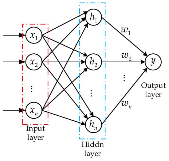
Figure 4. The structure diagram of the RBF neural network.

As seen in Figure 4, the RBF neural network is a three-layer feedforward network, which includes an input layer, a hidden layer and an output layer. Based on the Gaussian basis function, the RBF neural network can approximate the uncertain terms without the need for complex mathematical theoretical analysis. The expression of the RBF neural network could be designed as follows:

$$\left\{\begin{array}{l}{f}_{f_{j}u}(u_{f_j},v_{f_j},r_{f_j})=W_{f_{j}u}^{\ast T}h(z_{f_j})+{\delta }_{1f_j} , {\delta }_{1f_j}<{\delta }_{f_{j}U}\\ f_{f_{j}r}(u_{f_j},v_{f_j},r_{f_j})=W_{f_{j}r}^{\ast T}h(z_{f_j})+{\delta }_{2f_j} , {\delta }_{2f_j}<{\delta }_{f_{j}R}\\ h({\mathit{z}}_{f_j})=\exp (-{‖z_{f_j}-c_k‖}^2/2b_k^2), b_k>0, (k=1,2,\cdots ,n)\end{array}\right.$$

(25)

where ${\delta }_{1f_j}$ and ${\delta }_{2f_j}$ are the approximation errors of the neural network. ${\delta }_{f_{j}U}>0$ and ${\delta }_{f_{j}R}>0$ are the upper bounds of ${\delta }_{1f_j}$ and ${\delta }_{2f_j}$. $z_{f_j}={[u_{f_j},v_{f_j},r_{f_j}]}^T$ is the input vector of the RBF neural network, $h(z_{f_j})={[h_1(z_{f_j}),h_2(z_{f_j}),\cdots ,h_n(z_{f_j})]}^T$ represents the radial basis function vector of the neural network. $b_k$ is the width of the Gaussian basis function. The positive integer $k$ represents the $k^{\mathrm{th}}$ node in the hidden layer of the neural network.$c_k={[c_1,c_2,\cdots ,c_n]}^T\in R^n$ denotes the center value of the $k^{\mathrm{th}}$ hidden neuron. $W_{f_{j}u}^{\ast }={[w_{f_{j}u,1}^{\ast },w_{f_{j}u,2}^{\ast },\cdots ,w_{f_{j}u,n}^{\ast }]}^T\in R^n$ and $W_{f_{j}r}^{\ast }={[w_{f_{j}r,1}^{\ast },w_{f_{j}r,2}^{\ast },\cdots ,w_{f_{j}r,n}^{\ast }]}^T\in R^n$ are the weights associated with the $k^{\mathrm{th}}$ hidden neuron, which are designed as follows:

$$\left\{\begin{array}{l}{W}_{f_{j}u}^{\ast }=\underset{W\in R^n}{\mathrm{argmin}}\left\{\underset{z_{f_j}\in \mathsf{\Omega }}{\sup }\left|f_{f_{j}u}(u_{f_j},v_{f_j},r_{f_j})-W_{f_{j}u}^{T}h(z_{f_j})\right|\right\}\\ W_{f_{j}r}^{\ast }=\underset{W\in R^n}{\mathrm{argmin}}\left\{\underset{z_{f_j}\in \mathsf{\Omega }}{\sup }\left|f_{f_{j}r}(u_{f_j},v_{f_j},r_{f_j})-W_{f_{j}r}^{T}h(z_{f_j})\right|\right\}\end{array}\right.$$

(26)

Since $W_{f_{j}u}^{\ast }$ and $W_{f_{j}r}^{\ast }$ are often unattainable in practical applications, the estimated values ${\stackrel{\wedge }{W}}_{f_{j}u}$ and ${\stackrel{\wedge }{W}}_{f_{j}r}$ are designed to replace $W_{f_{j}u}^{\ast }$ and $W_{f_{j}r}^{\ast }$. Combining this with Equations (15) and (24), the surge force and the yaw moment of the $j^{\mathrm{th}}$ follower USV could be rewritten as follows:

$$\left\{\begin{array}{l}{\tau }_{f_{j}u}=m_{1j}[-{\stackrel{\wedge }{f}}_{f_{j}u}(u_{f_j},v_{f_j},r_{f_j})+{\dot{\beta }}_{f_{j}u}-{\lambda }_{1f_j}{u}_{f_{j}e}-{\epsilon }_{1f_j}\tanh (s_{1f_j})-{\sigma }_{1f_j}{s}_{1f_j}]\\ {\tau }_{r_j}={\displaystyle \frac{m_{3j}}{{\alpha }_{f_{j}u}}}[-{\ddot{v}}_{f_j}-{\lambda }_{2f_j}({\dot{v}}_{f_j}-{\dot{\beta }}_{f_{j}v})-{\lambda }_{3_j}(v_{f_j}-{\beta }_{f_{j}v})-r_{f_j}{\dot{\beta }}_{f_{j}u}\\ \hspace{1em}\hspace{1em}+{\dot{g}}_{f_j}-{\epsilon }_{2f_j}\tan \mathrm{h}(s_{2f_j})-{\sigma }_{2f_j}{s}_{2f_j}]-m_{3j}{\stackrel{\wedge }{f}}_{f_{j}r}(u_{f_j},v_{f_j},r_{f_j})\end{array}\right.$$

(27)

where ${\stackrel{\wedge }{f}}_{f_{j}u}(u_{f_j},v_{f_j},r_{f_j})=\stackrel{\wedge }{W_{f_{j}u}^T}h({\mathit{z}}_{f_j})$ is the estimated value of $f_{f_{j}u}(u_{f_j},v_{f_j},r_{f_j})$ and ${\stackrel{\wedge }{f}}_{f_{j}r}(u_{f_j},v_{f_j},r_{f_j})=\stackrel{\wedge }{W_{f_{j}r}^T}h(z_{f_j})$ is the estimated value of $f_{f_{j}r}(u_{f_j},v_{f_j},r_{f_j})$.

Meanwhile, to simplify the calculation, the MLP algorithm is utilized to substitute for online weight in a single-parameter form. Specifically, ${‖W_{f_{j}u}^{\ast }‖}^2$ and ${‖W_{f_{j}r}^{\ast }‖}^2$ could be designed as follows:

$$\left\{\begin{array}{l}{\varphi }_{1f_j}={‖W_{f_{j}u}^{\ast }‖}^2\\ {\varphi }_{2f_j}={‖W_{f_{j}r}^{\ast }‖}^2\end{array}\right.$$

(28)

where ${\varphi }_{1f_j}$ and ${\varphi }_{2f_j}$ are positive constants. And by defining ${\widehat{\varphi }}_{1f_j}$ and ${\widehat{\varphi }}_{2f_j}$ as the estimated value of ${\varphi }_{1f_j}$ and ${\varphi }_{2f_j}$, the adaptive parameters could be designed as follows:

$$\left\{\begin{array}{l}{\stackrel{·}{\widehat{\varphi }}}_{1f_j}={\zeta }_{1f_j}(s_{1f_j}^2{h}_{f_j}^T{h}_{f_j}/2-{\gamma }_{1f_j}{\widehat{\varphi }}_{1f_j})\\ {\stackrel{·}{\widehat{\varphi }}}_{2f_j}={\zeta }_{2f_j}(s_{2f_j}^2{h}_{f_j}^T{h}_{f_j}/2-{\gamma }_{2f_j}{\widehat{\varphi }}_{2f_j})\end{array}\right.$$

(29)

where ${\zeta }_{1f_j},{\zeta }_{2f_j},{\gamma }_{1f_j},{\gamma }_{2f_j}$ are positive numbers.

Combining this with Equations (27) and (29), the surge force and the yaw moment of the $j^{\mathrm{th}}$ follower USV could be designed as follows:

$$\left\{\begin{array}{l}{\tau }_{f_{j}u}=m_{1j}[-s_{1f_j}{\widehat{\varphi }}_{1f_j}{h}_{f_j}^T{h}_{f_j}/2+{\dot{\beta }}_{f_{j}u}-{\lambda }_{1f_j}{u}_{f_{j}e}-{\epsilon }_{1f_j}\tanh (s_{1f_j})-{\sigma }_{1f_j}{s}_{1f_j}]\\ {\tau }_{r_j}={\displaystyle \frac{m_{3j}}{{\alpha }_{f_{j}u}}}[-{\ddot{v}}_{f_j}-{\lambda }_{2f_j}({\dot{v}}_{f_j}-{\dot{\beta }}_{f_{j}v})-{\lambda }_{3_j}(v_{f_j}-{\beta }_{f_{j}v})-r_{f_j}{\dot{\beta }}_{f_{j}u}\\ \hspace{1em}+{\dot{g}}_{f_j}-{\epsilon }_{2f_j}\tan \mathrm{h}(s_{2f_j})-{\sigma }_{2f_j}{s}_{2f_j}]-m_{3j}{s}_{2f_j}{\widehat{\varphi }}_{2f_j}{h}_{f_j}^T{h}_{f_j}/2\end{array}\right.$$

(30)

4. Stability Analysis

To verify the stability of the designed controller, combining with the errors in sliding mode controller design and estimation error of the RBF neural network, the Lyapunov function could be designed as follows:

$$\left\{\begin{array}{l}{V}_{2f_j}=s_{1f_j}^2/2+s_{2f_j}^2/2+y_{f_{j}u}^2/2+y_{f_{j}v}^2/2+{\tilde{\varphi }}_{1f_j}^2/(2{\zeta }_{1f_j})+{\tilde{\varphi }}_{2f_j}^2/(2{\zeta }_{2f_j})\\ y_{f_{j}u}={\beta }_{f_{j}u}-{\alpha }_{f_{j}u}, y_{f_{j}v}={\beta }_{f_{j}v}-{\alpha }_{f_{j}v}\\ {\tilde{\varphi }}_{1f_j}={\varphi }_{1f_j}-{\widehat{\varphi }}_{1f_j}, {\tilde{\varphi }}_{2f_j}={\varphi }_{2f_j}-{\widehat{\varphi }}_{2f_j}\end{array}\right.$$

(31)

Combining this with Equations (13), (14), (22), (24) and (31), the derivation of the Lyapunov function $V_{2f_j}$ could be presented as follows:

$$\begin{array}{cc}{\dot{V}}_{2f_j}& =s_{1f_j}{\dot{s}}_{1f_j}+s_{2f_j}{\dot{s}}_{2f_j}+y_{f_{j}u}{\dot{y}}_{f_{j}u}+y_{f_{j}v}{\dot{y}}_{f_{j}v}-{\tilde{\varphi }}_{1f_j}{\dot{\widehat{\varphi }}}_{1f_j}/{\zeta }_{1f_j}-{\tilde{\varphi }}_{2f_j}{\dot{\widehat{\varphi }}}_{2f_j}/{\zeta }_{2f_j}\hfill \\ & =s_{1f_j}[{{\mathit{W}}_{f_{j}u}^{\ast }}^T\mathit{h}({\mathit{z}}_{f_j})+{\delta }_{1f_j}-s_{1f_j}{\widehat{\varphi }}_{1f_j}{\mathit{h}}_{f_j}^T{\mathit{h}}_{f_j}/2-{\epsilon }_{1f_j}\tanh (s_{1f_j})-{\sigma }_{1f_j}{s}_{1f_j}]+s_2[{{\mathit{W}}_{f_{j}r}^{\ast }}^T\mathit{h}({\mathit{z}}_{f_k})+{\delta }_{2f_j}\\ & \hspace{1em}-s_{2f_j}{\widehat{\varphi }}_{2f_j}{\mathit{h}}_{f_j}^T{\mathit{h}}_{f_j}/2-{\epsilon }_{2f_j}\tanh (s_{2f_j})-{\sigma }_{2f_j}{s}_{2f_j}]+y_{f_{j}u}({\dot{\beta }}_{f_{j}u}-{\dot{\alpha }}_{f_{j}u})+y_{f_{j}v}({\dot{\beta }}_{f_{j}v}-{\dot{\alpha }}_{f_{j}v})\hfill \\ & -{\tilde{\varphi }}_{1f_j}{\dot{\widehat{\varphi }}}_{1f_j}/{\zeta }_{1f_j}-{\tilde{\varphi }}_{2f_j}{\dot{\widehat{\varphi }}}_{2f_j}/{\zeta }_{2f_j}\hfill \\ & =-{\sigma }_{1f_j}{s}_{1f_j}^2-{\sigma }_{2f_j}{s}_{2f_j}^2+s_{1f_j}{\delta }_{1f_j}+s_{2f_j}{\delta }_{2f_j}-s_{1f_j}{\epsilon }_{1f_j}\tanh (s_{1f_j})-s_{2f_j}{\epsilon }_{2f_j}\tanh (s_{2f_j})\hfill \\ & \hspace{1em}+s_{1f_j}{{\mathit{W}}_{f_{j}r}^{\ast }}^T\mathit{h}({\mathit{z}}_{f_j})-s_{1f_j}^2{\widehat{\varphi }}_{1f_j}{\mathit{h}}_{f_j}^T{\mathit{h}}_{f_j}/2+s_{2f_j}{{\mathit{W}}_{f_{j}r}^{\ast }}^T\mathit{h}({\mathit{z}}_{f_j})-s_{2f_j}^2{\widehat{\varphi }}_{2f_j}{\mathit{h}}_{f_j}^T{\mathit{h}}_{f_j}/2+y_{f_{j}u}[-B_{1f_j}{\beta }_{f_{j}u}\hfill \\ & \hspace{1em}+(C_{1f_j}-{\beta }_{f_{j}u})f({\alpha }_{f_{j}u})-(D_{1f_j}+{\beta }_{f_{j}u})g({\alpha }_{f_{j}u})-{\dot{\alpha }}_{f_{j}u}]+y_{f_{j}v}[-B_{2f_j}{\beta }_{f_{j}v}+(C_{2f_j}-{\beta }_{f_{j}v})f({\alpha }_{f_{j}v})\hfill \\ & \hspace{1em}-(D_{2f_j}+{\beta }_{f_{j}v})g({\alpha }_{f_{j}v})-{\dot{\alpha }}_{f_{j}v}]-{\tilde{\varphi }}_{1f_j}{\dot{\widehat{\varphi }}}_{1f_j}/{\zeta }_{1f_j}-{\tilde{\varphi }}_{2f_j}{\dot{\widehat{\varphi }}}_{2f_j}/{\zeta }_{2f_j}\hfill \\ & \le -{\sigma }_{1f_j}{s}_{1f_j}^2-{\sigma }_{2f_j}{s}_{2f_j}^2+s_{1f_j}{\delta }_{1f_j}+s_{2f_j}{\delta }_{2f_j}-{\epsilon }_{1f_j}\left|s_{1f_j}\right|-{\epsilon }_{2f_j}\left|s_{2f_j}\right|+s_{1f_j}{{\mathit{W}}_{f_{j}r}^{\ast }}^T\mathit{h}({\mathit{z}}_{f_j})\hfill \\ & \hspace{1em}-s_{1f_j}^2{\widehat{\varphi }}_{1f_j}{\mathit{h}}_{f_j}^T{\mathit{h}}_{f_j}/2+s_{2f_j}{{\mathit{W}}_{f_{j}r}^{\ast }}^T\mathit{h}({\mathit{z}}_{f_j})-s_{2f_j}^2{\widehat{\varphi }}_{2f_j}{\mathit{h}}_{f_j}^T{\mathit{h}}_{f_j}/2+y_{f_{j}u}[-B_{1f_j}{\beta }_{f_{j}u}+(C_{1f_j}-{\beta }_{f_{j}u})f({\alpha }_{f_{j}u})\hfill \\ & \hspace{1em}-(D_{1f_j}+{\beta }_{f_{j}u})g({\alpha }_{f_{j}u})-{\dot{\alpha }}_{f_{j}u}]+y_{f_{j}v}[-B_{2f_j}{\beta }_{f_{j}v}+(C_{2f_j}-{\beta }_{f_{j}v})f({\alpha }_{f_{j}v})-(D_{2f_j}+{\beta }_{f_{j}v})g({\alpha }_{f_{j}v})\hfill \\ & \hspace{1em}-{\dot{\alpha }}_{f_{j}v}]-{\tilde{\varphi }}_{1f_j}{\dot{\widehat{\varphi }}}_{1f_j}/{\zeta }_{1f_j}-{\tilde{\varphi }}_{2f_j}{\dot{\widehat{\varphi }}}_{2f_j}/{\zeta }_{2f_j}\hfill \end{array}$$

(32)

According to Equations (25) and (28), the following inequalities could be presented as follows:

$$\left\{\begin{array}{l}{s}_{1f_j}{\delta }_{1f_j}\le s_{1f_j}^2/2+{\delta }_{1f_j}^2/2\le s_{1f_j}^2/2+{\delta }_{f_{j}U}^2/2\\ s_{2f_j}{\delta }_{2f_j}\le s_{2f_j}^2/2+{\delta }_{2f_j}^2/2\le s_{2f_j}^2/2+{\delta }_{f_{j}R}^2/2\\ 2s_{1f_j}{{\mathit{W}}_{f_{j}u}^{\ast }}^T{h}_{f_j}\le s_{1f_j}^2{‖{\mathit{W}}_{f_{j}u}^{\ast }‖}^2{‖h_{f_j}‖}^2+1=s_{1f_j}^2{\varphi }_{1f_j}{h}_{f_j}^T{h}_{f_j}+1\\ 2s_{2f_j}{{\mathit{W}}_{f_{j}u}^{\ast }}^T{h}_{f_j}\le s_{2f_j}^2{‖{\mathit{W}}_{f_{j}r}^{\ast }‖}^2{‖h_{f_j}‖}^2+1=s_{2f_j}^2{\varphi }_{2f_j}{h}_{f_j}^T{h}_{f_j}+1\end{array}\right.$$

(33)

As seen from Equations (13) and (22), there exists $f({\alpha }_{f_{j}u})\ge 0, f({\alpha }_{f_{j}v})\ge 0$ and $g({\alpha }_{f_{j}u})\ge 0, g({\alpha }_{f_{j}v})\ge 0$, and then Equation (32) could be simplified as follows:

$$\begin{array}{l}{\dot{V}}_{2f_j}\le -{\sigma }_{1f_j}{s}_{1f_j}^2-{\sigma }_{2f_j}{s}_{2f_j}^2+s_{1f_j}^2/2+{\delta }_{f_{j}U}^2/2+s_{2f_j}^2/2+{\delta }_{f_{j}R}^2/2-{\epsilon }_{1f_j}\left|s_{1f_j}\right|-{\epsilon }_{2f_j}\left|s_{2f_j}\right|\\ \hspace{1em}+s_{1f_j}{\tilde{\varphi }}_{1f_j}{h}_{f_j}^T{h}_{f_j}/2+s_{2f_j}{\tilde{\varphi }}_{2f_j}{h}_{f_j}^T{h}_{f_j}/2+1+y_{f_{j}u}(-B_{f_{j}u}{\beta }_{f_{j}u}+C_{1f_j}{\alpha }_{f_{j}u}-{\dot{\alpha }}_{f_{j}u})\\ \hspace{1em}+y_{f_{j}v}(-B_{f_{j}v}{\beta }_{f_{j}v}+C_{2f_j}{\alpha }_{f_{j}v}-{\dot{\alpha }}_{f_{j}v})-{\tilde{\varphi }}_{1f_j}{\dot{\widehat{\varphi }}}_{1f_j}/{\zeta }_{1f_j}-{\tilde{\varphi }}_{2f_j}{\dot{\widehat{\varphi }}}_{2f_j}/{\zeta }_{2f_j}\\ \mathrm{s}.\mathrm{t}. \left\{\begin{array}{l}{C}_{1f_j}=D_{1f_j},C_{2f_j}=D_{2f_j}\\ B_{f_{j}u}=B_{1f_j}+f({\alpha }_{f_{j}u})+g({\alpha }_{f_{j}u})>0\\ B_{f_{j}v}=B_{2f_j}+f({\alpha }_{f_{j}v})+g({\alpha }_{f_{j}v})>0\end{array}\right.\end{array}$$

(34)

Combining this with Equation (29), and assuming $B_{f_{j}u}=C_{1f_j}$ and $B_{f_{j}v}=C_{2f_j}$, then the Equation (34) can be written as follows:

$$\begin{array}{cc}{\dot{V}}_{2f_j}& \le -(2{\sigma }_{1f_j}-1)s_{1f_j}^2/2-(2{\sigma }_{2f_j}-1)s_{2f_j}^2/2+{\delta }_{f_{j}U}^2/2+{\delta }_{f_{j}R}^2/2+s_{1f_j}{\tilde{\varphi }}_{1f_j}{h}_{f_j}^T{h}_{f_j}/2\hfill \\ & +s_{2f_j}{\tilde{\varphi }}_{2f_j}{h}_{f_j}^T{h}_{f_j}/2+1-B_{f_{j}u}{y}_{f_{j}u}^2-y_{f_{j}u}{\dot{\alpha }}_{f_{j}u}-B_{f_{j}v}{y}_{f_{j}v}^2-y_{f_{j}v}{\dot{\alpha }}_{f_{j}v}\hfill \\ & -{\tilde{\varphi }}_{1f_j}(s_{1f_j}{h}_{f_j}^T{h}_{f_j}/2-{\gamma }_{1f_j}{\widehat{\varphi }}_{1f_j})-{\tilde{\varphi }}_{2f_j}(s_{2f_j}{h}_{f_j}^T{h}_{f_j}/2-{\gamma }_{2f_j}{\widehat{\varphi }}_{2f_j})\hfill \\ & \le -(2{\sigma }_{1f_j}-1)s_{1f_j}^2/2-(2{\sigma }_{2f_j}-1)s_{2f_j}^2/2+{\delta }_{f_{j}U}^2/2+{\delta }_{f_{j}R}^2/2-B_{f_{j}u}{y}_{f_{j}u}^2-y_{f_{j}u}{\dot{\alpha }}_{f_{j}u}-B_{f_{j}v}{y}_{f_{j}v}^2\hfill \\ & \hspace{1em}-y_{f_{j}v}{\dot{\alpha }}_{f_{j}v}+{\gamma }_{1f_j}{\tilde{\varphi }}_{1f_j}{\widehat{\varphi }}_{1f_j}+{\gamma }_{2f_j}{\tilde{\varphi }}_{2f_j}{\widehat{\varphi }}_{2f_j}\hfill \end{array}$$

(35)

Since the desired trajectories of USVs are smooth and bounded, the control inputs and velocities of USVs are bounded, it leads to:

$$\left\{\begin{array}{l}-y_{f_{j}u}{\dot{\alpha }}_{f_{j}u}\le {\displaystyle \frac{{\sigma }_{f_{j}u}}{2}}{y}_{f_{j}u}^2+{\displaystyle \frac{1}{2{\sigma }_{f_{j}u}}}{\dot{\alpha }}_{f_{j}u}^2\le {\displaystyle \frac{{\sigma }_{f_{j}u}}{2}}{y}_{f_{j}u}^2+{\displaystyle \frac{1}{2{\sigma }_{f_{j}u}}}{\dot{U}}_{f_j\max }^2\\ -y_{f_{j}v}{\dot{\alpha }}_{f_{j}v}\le {\displaystyle \frac{{\sigma }_{f_{j}v}}{2}}{y}_{f_{j}v}^2+{\displaystyle \frac{1}{2{\sigma }_{f_{j}v}}}{\dot{\alpha }}_{f_{j}v}^2\le {\displaystyle \frac{{\sigma }_{f_{j}v}}{2}}{y}_{f_{j}v}^2+{\displaystyle \frac{1}{2{\sigma }_{f_{j}v}}}{\dot{V}}_{f_j\max }^2\\ 2{\tilde{\varphi }}_{1f_j}{\widehat{\varphi }}_{1f_j}=({\varphi }_{1f_j}-{\widehat{\varphi }}_{1f_j}){\widehat{\varphi }}_{1f_j}+{\tilde{\varphi }}_{1f_j}({\varphi }_{1f_j}-{\tilde{\varphi }}_{1f_j})={\varphi }_{1f_j}^2-{\widehat{\varphi }}_{1f_j}^2-{\tilde{\varphi }}_{1f_j}^2\le {\varphi }_{1f_j}^2-{\tilde{\varphi }}_{1f_j}^2\\ 2{\tilde{\varphi }}_{2f_j}{\widehat{\varphi }}_{2f_j}=({\varphi }_{2f_j}-{\widehat{\varphi }}_{2f_j}){\widehat{\varphi }}_{2f_j}+{\tilde{\varphi }}_{2f_j}({\varphi }_{2f_j}-{\tilde{\varphi }}_{2f_j})={\varphi }_{2f_j}^2-{\widehat{\varphi }}_{2f_j}^2-{\tilde{\varphi }}_{2f_j}^2\le {\varphi }_{2f_j}^2-{\tilde{\varphi }}_{2f_j}^2\end{array}\right.$$

(36)

where ${\dot{U}}_{f_j\max }$ is the maximum value of ${\dot{\alpha }}_{f_{j}u}$ and ${\dot{V}}_{f_j\max }$ is the maximum value of ${\dot{\alpha }}_{f_{j}v}$.

Combining this with Equation (36), Equation (35) could be simplified as follows:

$$\begin{array}{cc}{\dot{V}}_{2f_j}& \le -(2{\sigma }_{1f_j}-1)s_{1f_j}^2/2-(2{\sigma }_{2f_j}-1)s_{2f_j}^2/2-(B_{f_{j}u}-{\sigma }_{f_{j}u}/2)y_{f_{j}u}^2-(B_{f_{j}v}-{\sigma }_{f_{j}v}/2)y_{f_{j}v}^2\hfill \\ & -{\gamma }_{1f_j}{\tilde{\varphi }}_{1f_j}^2/2-{\gamma }_{2f_j}{\tilde{\varphi }}_{2f_j}^2/2+{\delta }_{f_{j}U}^2/2+{\delta }_{f_{j}R}^2/2+{\dot{U}}_{f_j\max }^2/(2{\sigma }_{f_{j}u})+{\dot{V}}_{f_j\max }^2/(2{\sigma }_{f_{j}v})\hfill \\ & +{\gamma }_{1f_j}{\varphi }_{1f_j}^2/2+{\gamma }_{2f_j}{\varphi }_{2f_j}^2/2\hfill \\ & \le \mu V_{2f_j}+C_3\hfill \\ \mathrm{s}.\mathrm{t}. & \left\{\begin{array}{l}\mu =\min \{(2{\sigma }_{1f_j}-1)/2,(2{\sigma }_{2f_j}-1)/2,B_{f_{j}u}-{\sigma }_{f_{j}u}/2,B_{f_{j}v}-{\sigma }_{f_{j}v}/2,{\gamma }_{1f_j}/2,{\gamma }_{2f_j}/2\}\\ C_3={\delta }_{f_{j}U}^2/2+{\delta }_{f_{j}R}^2/2+{\dot{U}}_{f_j\max }^2/(2{\sigma }_{f_{j}u})+{\dot{V}}_{f_j\max }^2/(2{\sigma }_{f_{j}v})+{\gamma }_{1f_j}{\varphi }_{1f_j}^2/2+{\gamma }_{2f_j}{\varphi }_{2f_j}^2/2+1\\ B_{f_{j}u}-{\sigma }_{f_{j}u}/2>0,B_{f_{j}v}-{\sigma }_{f_{j}v}/2>0\end{array}\right.\hfill \end{array}$$

(37)

By solving Equation (37), it leads to

$$0\le V_{2f_j}(t)\le C_3/\mu +[V_{2f_j}(0)-C_3/\mu ]e^{-\mu t}$$

(38)

According to Equation (38), $V_{2f_j}(t)$ converges within a ball of radius $C_3/\mu$, so that it is ultimately uniformly bounded. By choosing appropriate control parameters, the convergent limit of $V_{2f_i}(t)$ is inclined to zero. And it can be demonstrated that the designed sliding mode controller finally tends to be stable at $t\to \infty$ with $x_{f_{j}e}\to 0$, $y_{f_{j}e}\to 0$, $u_{f_{j}e}\to 0$ and $v_{f_{j}e}\to 0$.

5. Computer Simulation

To highlight the advantages of the proposed bio-inspired sliding mode control (bio-SMC) method and the radial basis function neural network (RBF), four experiment cases including circular trajectory, straight line trajectory, sinusoidal trajectory and combination trajectory of straight line and circle are set in this section, and three USVs are taken as an example, where one is the leader USV, and the other two are the follower USVs. The USV model parameters are presented by [28], and the specific parameters are shown in Table 1.

Table 1. USVs model parameters.

Parameter	Value (Unit)	Parameter	Value (Unit)
$m_{1j}$	25.8 kg	$d_{1j}$	12 kg/s
$m_{2j}$	33.8 kg	$d_{2j}$	17 kg/s
$m_{3j}$	2.76 kg.m2	$d_{3j}$	0.5 kg.m2/s

The simulation time interval is 0.1 s and the external environmental disturbance is $d_j={[2\sin (0.1t),0.2\sin (0.01t),\sin (0.1t)]}^T$. The model uncertainties of USV are considered as $\Delta f_j={[-0.2d_{1j}{u}_j^2/m_{1j}-0.1d_{1j}{u}_j^3/m_{1j},-0.2d_{2j}{v}_j^2/m_{2j}-0.1d_{2j}{v}_j^3/m_{2j},-0.2d_{3j}{r}_j^2/m_{3j}-0.1d_{3j}{r}_j^3/m_{3j}]}^T$.

Considering the constraints of the actuators on USVs in practical engineering, limitations are set on the control input, especially described as follows:

$$\left\{\begin{array}{l}{\tau }_{u\max }=50 \mathrm{N}, {\tau }_{r\max }=30 \mathrm{N}\cdot \mathrm{m}\\ d{\tau }_{u\max }=50 \mathrm{N}/\mathrm{s}, d{\tau }_{r\max }=50 \mathrm{N}\cdot \mathrm{m}/\mathrm{s}\end{array}\right.$$

(39)

In order to intuitively describe the tracking effect of the USV, the longitudinal position error of the USV is defined as $x_{ej}=\left|x_j-x_{dj}\right|$ and lateral position error of the USV is defined as $y_{ej}=\left|y_j-y_{dj}\right|$. And the longitudinal velocity error and lateral velocity error are $u_{je}=u_j-{\alpha }_{ju}$ and $v_{je}=v_j-{\alpha }_{jv}$.

• Case 1. Circular trajectory

The desired circular trajectory of the leader USV is described as: $x_d=30\sin 0.05t$, $y_d=-30\cos 0.05t$. The initial state information for each USV in the formation system is presented in Table 2.

Table 2. USVs initial state (Case 1).

Parameter	Leader USV	Follower USV1	Follower USV2
$\eta$	${[-5(m),-35(m),45{(}^{\circ })]}^T$	${[-6(m),-32(m),45{(}^{\circ })]}^T$	${[-6(m),-42(m),45{(}^{\circ })]}^T$
$v$	${[0,0,0]}^T$	${[0,0,0]}^T$	${[0,0,0]}^T$
$L$		${[0(m),5(m)]}^T$	${[0(m),-5(m)]}^T$

The input of the RBF neural network ${\stackrel{\wedge }{f}}_{f_{j}u}(u_{f_j},v_{f_j},r_{f_j})$ is 3; the number of nodes in the hidden layer is 9; the width of the Gaussian basis function is 2 and the vector values for the center points are normally distributed in the range of [−15, 15]. The input of the RBF neural network ${\stackrel{\wedge }{f}}_{f_{j}r}(u_{f_j},v_{f_j},r_{f_j})$ is 3; the number of nodes in the hidden layer is 9; the width of the Gaussian basis function is 4 and the vector values for the center points are normally distributed in the range of [−0.3, 0.3]. The controller parameters are presented in Table 3.

Table 3. USVs controller parameters (Case 1).

Parameter	Leader USV	Follower USV1	Follower USV2
$C$	50	40	50
$k_1$	3	2	3
$k_2$	5	2	6.5
${\lambda }_1$	0.002	0.002	0.002
${\lambda }_2$	6	4.5	5
${\lambda }_3$	0.05	0.05	0.05
${\epsilon }_1$	0.01	0.001	0.01
${\epsilon }_2$	0.01	0.01	0.01
${\sigma }_1$	0.5	0.5	0.5
${\sigma }_2$	0.01	0.01	0.01
$B_1$	2	1.5	2
$B_2$	4	4	4
$C_1{,\mathrm{D}}_1$	3.4	2.5	3.75
$C_2{,\mathrm{D}}_2$	4	4	4
${\zeta }_1$	20	60	10
${\zeta }_2$	0.01	0.015	0.015
${\gamma }_1$	0.0005	0	0
${\gamma }_2$	0.001	0.001	0.001

The simulation results of Case 1 are shown in Figure 5, Figure 6, Figure 7, Figure 8, Figure 9, Figure 10 and Figure 11.

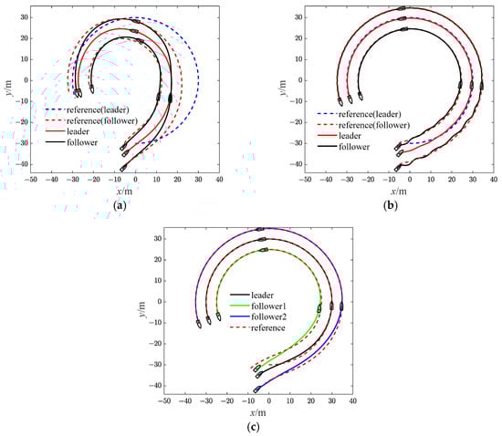
Figure 5. Diagrams of USVs trajectory (Case 1). (a)with SMC; (b) with SMC and RBF; (c) with bio-SMC and RBF.

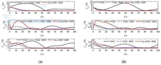
Figure 6. Diagrams of USVs’ tracking error (Case 1). (a) longitudinal position error; (b) lateral position error.

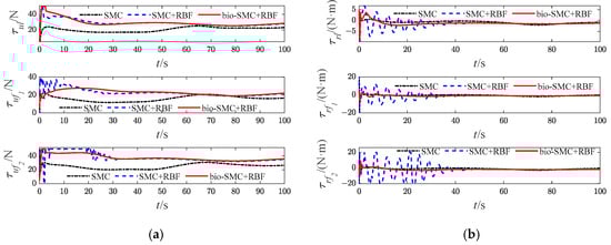
Figure 7. Diagrams of USVs’ control input signals (Case 1). (a) surge force; (b) yaw moment.

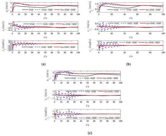
Figure 8. Diagrams of USVs’ velocity variables (Case 1). (a) Leader USV; (b) Follower USV1; (c) Follower USV2.

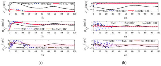
Figure 9. Diagrams of USVs’ virtual velocity variables (Case 1). (a) longitudinal virtual velocity; (b) lateral virtual velocity.

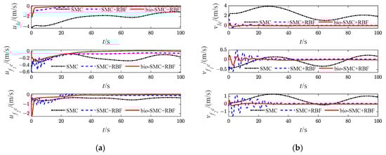
Figure 10. Diagrams of USVs’ velocity error (Case 1). (a) longitudinal velocity error; (b) lateral velocity error.

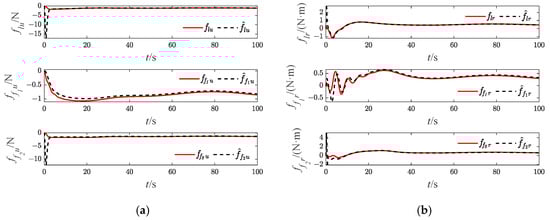
Figure 11. Approximation results of USVs (Case 1). (a) surge dynamic damping; (b) yaw dynamic damping.

• Case 2. Straight line trajectory

The desired straight line trajectory of the leader USV is described as: $x_d=t$, $y_d=t$. The initial state information for each USV in the formation system is presented in Table 4.

Table 4. USVs initial state (Case 2).

Parameter	Leader USV	Follower USV1	Follower USV2
$\eta$	${[-5(m),-2(m),0]}^T$	${[-12(m),-15(m),90{(}^{\circ })]}^T$	${[-4(m),-20(m),-90{(}^{\circ })]}^T$
$v$	${[0,0,0]}^T$	${[0,0,0]}^T$	${[0,0,0]}^T$
$L$		${[-5(m),10(m)]}^T$	${[-5(m),-10(m)]}^T$

The parameters of the RBF neural network are same as for Case 1, besides the width of the Gaussian basis function, and the width of the Gaussian basis function is 2. The controller parameters are presented in Table 5.

Table 5. USVs’ controller parameters (Case 2).

Parameter	Leader USV	Follower USV1	Follower USV2
$C$	50	50	40
$k_1$	3.5	3.5	2
$k_2$	6	6	3
${\lambda }_1$	0.012	0.012	0.001
${\lambda }_2$	6.5	5	5
${\lambda }_3$	0.001	0.05	0.05
${\epsilon }_1$	0.05	0.05	0.05
${\epsilon }_2$	0.01	0.01	0.01
${\sigma }_1$	0.05	0.1	0.1
${\sigma }_2$	0.01	0.01	0.01
$B_1$	2.5	5.5	5.5
$B_2$	4	4	4
$C_1{,\mathrm{D}}_1$	4	7	7
$C_2{,\mathrm{D}}_2$	4	4	4
${\zeta }_1$	3	8	8
${\zeta }_2$	0.01	0.025	0.025
${\gamma }_1$	0.008	0.08	0.001
${\gamma }_2$	0.1	0.1	0.1

The simulation results of Case 2 are shown in Figure 12, Figure 13, Figure 14, Figure 15, Figure 16, Figure 17 and Figure 18.

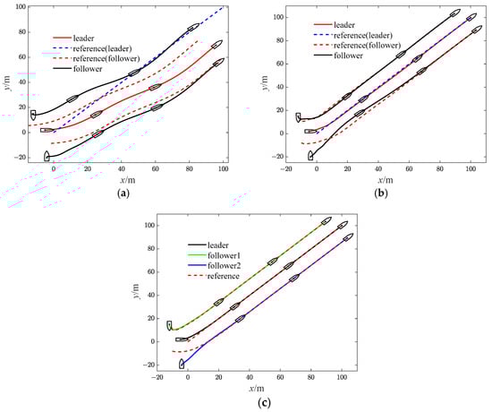
Figure 12. Diagrams of USVs’ trajectory (Case 2). (a)with SMC; (b) with SMC and RBF; (c) with bio-SMC and RBF.

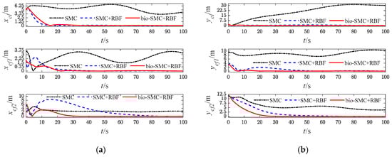
Figure 13. Diagrams of USVs’ tracking error (Case 2). (a) longitudinal position error; (b) lateral position error.

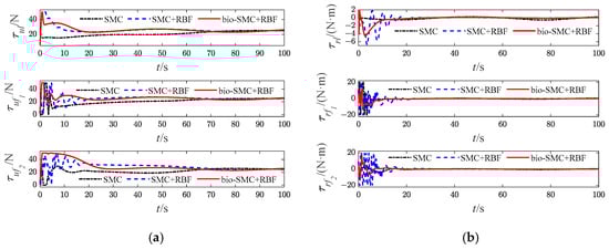
Figure 14. Diagrams of USVs’ control input signals (Case 2). (a) surge force; (b) yaw moment.

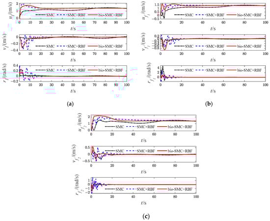
Figure 15. Diagrams of USVs’ velocity variables (Case 2). (a) Leader USV; (b) Follower USV1; (c) Follower USV2.

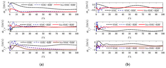
Figure 16. Diagrams of USVs’ virtual velocity variables (Case 2). (a) longitudinal virtual velocity; (b) lateral virtual velocity.

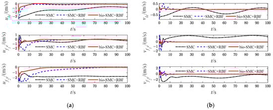
Figure 17. Diagrams of USVs’ velocity error (Case 2). (a) longitudinal velocity error; (b) lateral velocity error.

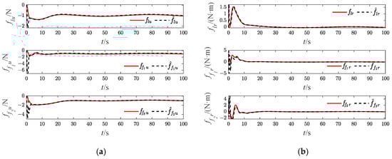
Figure 18. Approximation results of USVs’ (Case 2). (a) surge dynamic damping; (b) yaw dynamic damping.

• Case 3. Sinusoidal trajectory

The desired sinusoidal trajectory of the leader USV is described as $x_d=t$, $y_d=25\sin (0.05t)-35$. The initial state information for each USV in the formation system is presented in Table 6.

Table 6. USVs’ initial state (Case 3).

Parameter	Leader USV	Follower USV1	Follower USV2
$\eta$	${[-5(m),-35(m),45{(}^{\circ })]}^T$	${[-6(m),-32(m),45{(}^{\circ })]}^T$	${[-6(m),-42(m),45{(}^{\circ })]}^T$
$v$	${[0,0,0]}^T$	${[0,0,0]}^T$	${[0,0,0]}^T$
$L$		${[0(m),5(m)]}^T$	${[0(m),-5(m)]}^T$

The parameters of the RBF neural network are same as for Case 2, and the controller parameters are presented in Table 7.

Table 7. USVs’ controller parameters (Case 3).

Parameter	Leader USV	Follower USV1	Follower USV2
$C$	30	30	40
$k_1$	2	9.5	9
$k_2$	3.5	4	5
${\lambda }_1$	0.0001	0.0001	0.0001
${\lambda }_2$	1.2	1.2	1.2
${\lambda }_3$	0.001	0.01	0.001
${\epsilon }_1$	0.01	0.05	0.05
${\epsilon }_2$	0.01	0.01	0.01
${\sigma }_1$	0.02	0.01	0.01
${\sigma }_2$	0.1	0.01	0.01
$B_1$	4	4	4
$B_2$	4	6.7	7.75
$C_1{,\mathrm{D}}_1$	4	4	4
$C_2{,\mathrm{D}}_2$	4	4	4
${\zeta }_1$	1	0.01	0.1
${\zeta }_2$	0.015	0.01	0.006
${\gamma }_1$	0.0005	0.0005	0.0005
${\gamma }_2$	0.001	0.001	0.001

The simulation results of Case 3 are shown in Figure 19, Figure 20, Figure 21, Figure 22, Figure 23, Figure 24 and Figure 25.

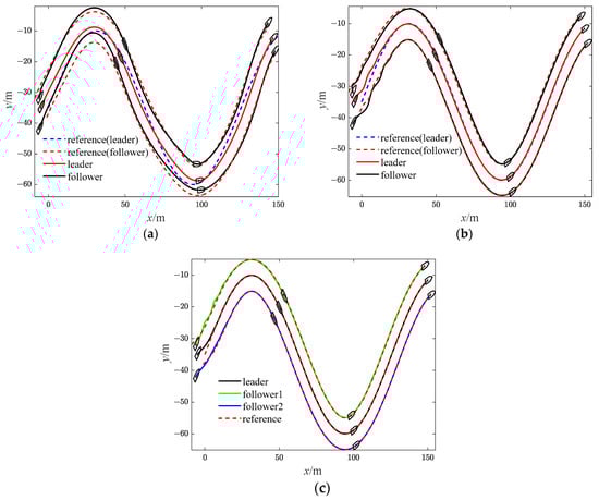
Figure 19. Diagrams of USVs’ trajectory (Case 3). (a)with SMC; (b) with SMC and RBF; (c) with bio-SMC and RBF.

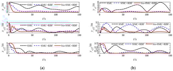
Figure 20. Diagrams of USVs’ tracking error (Case 3). (a) longitudinal position error; (b) lateral position error.

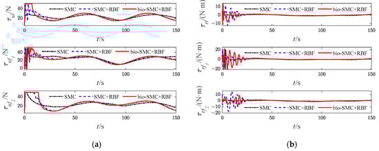
Figure 21. Diagrams of USVs’ control input signals (Case 3). (a) surge force; (b) yaw moment.

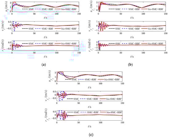
Figure 22. Diagrams of USVs’ velocity variables (Case 3). (a) Leader USV; (b) Follower USV1; (c) Follower USV2.

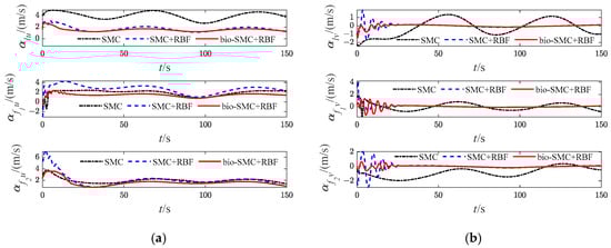
Figure 23. Diagrams of USVs’ virtual velocity variables (Case 3). (a) longitudinal virtual velocity; (b) lateral virtual velocity.

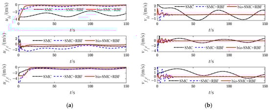
Figure 24. Diagrams of USVs’ velocity error (Case 3). (a) longitudinal velocity error; (b) lateral velocity error.

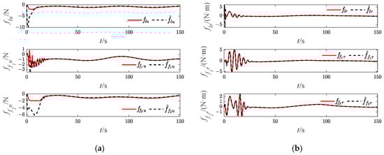
Figure 25. Approximation results of USVs’ (Case 3). (a) surge dynamic damping; (b) yaw dynamic damping.

• Case 4. Combination trajectory of straight line and circle

The desired sinusoidal trajectory of the leader USV is described as follows:

$$\left\{\begin{array}{l}{x}_d=t-90, y_d=-25, 0\le t<90 \mathrm{s}\\ x_d=25\sin (0.05(t-90)), y_d=25\cos (0.05(t-90)), t\ge 90 \mathrm{s}\end{array}\right.$$

The initial state information for each USV is presented in Table 8.

Table 8. USVs’ initial state (Case 4).

Parameter	Leader USV	Follower USV1	Follower USV2
$\eta$	${[-90(m),-30(m),0{(}^{\circ })]}^T$	${[-95(m),-20(m),0{(}^{\circ })]}^T$	${[-95(m),-40(m),0{(}^{\circ })]}^T$
$v$	${[0,0,0]}^T$	${[0,0,0]}^T$	${[0,0,0]}^T$
$L$		${[0(m),5(m)]}^T$	${[0(m),-5(m)]}^T$

The parameters of the RBF neural network are same as for Case 1, and the controller parameters are presented in Table 9.

Table 9. USVs’ controller parameters (Case 4).

Parameter	Leader USV	Follower USV1	Follower USV2
$C$	30	30	30
$k_1$	5	0.8	1.4
$k_2$	3	2	1.94
${\lambda }_1$	0.002	0.002	0.002
${\lambda }_2$	2.5	3.1	2
${\lambda }_3$	0.001	0.001	0.001
${\epsilon }_1$	0.01	0.01	0.01
${\epsilon }_2$	0.05	0.05	0.05
${\sigma }_1$	0.1	0.01	0.01
${\sigma }_2$	0.01	0.01	0.01
$B_1$	2.5	5.5	6
$B_2$	4	4	4
$C_1{,\mathrm{D}}_1$	4	6.7	7.75
$C_2{,\mathrm{D}}_2$	4	4	4
${\zeta }_1$	1	60	60
${\zeta }_2$	0.015	0.01	0.05
${\gamma }_1$	0.0005	0.0005	0.0005
${\gamma }_2$	0.001	0.0001	0.001

The simulation results of Case 4 are shown in Figure 26, Figure 27, Figure 28, Figure 29, Figure 30, Figure 31 and Figure 32.

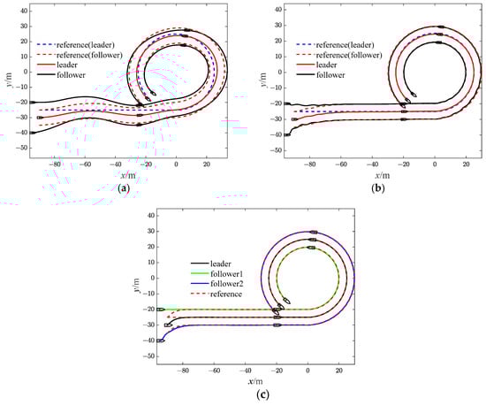
Figure 26. Diagrams of USVs’ trajectory (Case 4). (a) with SMC; (b) with SMC and RBF; (c) with bio-SMC and RBF.

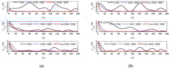
Figure 27. Diagrams of USVs’ tracking error (Case 4). (a) longitudinal position error; (b) lateral position error.

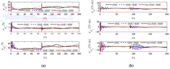
Figure 28. Diagrams of USVs’ control input signals (Case 4). (a) surge force; (b) yaw moment.

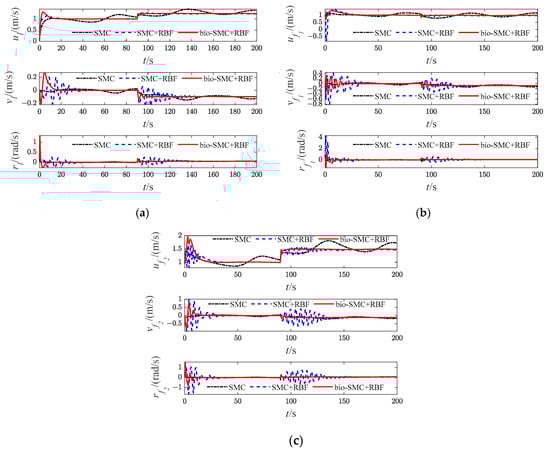
Figure 29. Diagrams of USVs’ velocity variables (Case 4). (a) Leader USV; (b) Follower USV1; (c) Follower USV2.

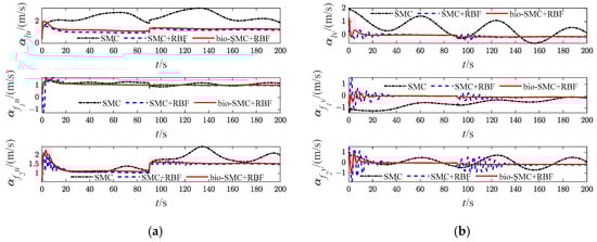
Figure 30. Diagrams of USVs’ virtual velocity variables (Case 4). (a) longitudinal virtual velocity; (b) lateral virtual velocity.

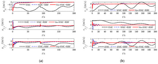
Figure 31. Diagrams of USVs’ velocity error (Case 4). (a) longitudinal velocity error; (b) lateral velocity error.

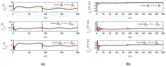
Figure 32. Approximation results of USVs’ (Case 4). (a) surge dynamic damping; (b) yaw dynamic damping.

The effectiveness of the RBF and the bio-inspired sliding mode control (bio-SMC) are analyzed through the above four experiment cases, in which Figure 5a, Figure 12a, Figure 19a and Figure 26a show the trajectory tracking results of the traditional sliding mode control (SMC) without RBF, while Figure 5b, Figure 12b, Figure 19b and Figure 26b indicate the formation trajectories with RBF. Through comparative analysis of these figures, USVs are able to track the desired trajectory with RBF under the influence caused by ocean disturbances and model uncertainties. Combining Figure 6, Figure 13, Figure 20 and Figure 27, after the formation system is stable, the tracking errors of USVs are generally greater than 1 m without RBF, but the tracking errors are far less than 0.5 m without RBF. Similarly, as seen from the velocity error plots, which include Figure 10, Figure 17, Figure 24 and Figure 31, the velocity errors of USVs are smaller with RBF. Meanwhile, according to Figure 11, Figure 18, Figure 25 and Figure 32, the RBF can accurately observe ocean disturbances and model uncertainties of USVs, and the effectiveness of RBF can be intuitively verified.

Then, as shown in Figure 5c, Figure 12c, Figure 19c and Figure 26c, which indicate the results of formation trajectories with bio-SMC and RBF, it is found that the fluctuation of the bio-SMC trajectory is smaller compared to Figure 5b, Figure 12b, Figure 19b and Figure 26b in the early stage of trajectory tracking. Meanwhile, as seen from Figure 9, Figure 16, Figure 23 and Figure 30, where the virtual velocity variables can be obtained, by utilizing bio-SMC, the virtual velocity changes become smoother within the first 30 s. Also, by analyzing Figure 8, Figure 15, Figure 22 and Figure 29, the bio-SMC has a significant effect on stabilizing these velocity variables within the first 30 s.

According to Figure 6, Figure 13, Figure 20 and Figure 27, the bio-SMC has no adverse effect on USVs’ trajectory tracking accuracy when the formation system is stable. Figure 7, Figure 14, Figure 21 and Figure 28 illustrate that within the first 30 s, the controllers of USVs designed by bio-SMC can obtain smoother control inputs. Therefore, based on the above analysis, the bio-SMC has better control capability compared to the traditional sliding mode control.

6. Conclusions

To address the cooperative formation control problem of underactuated USVs with external environmental disturbances and model uncertainties, a bio-inspired sliding mode control (bio-SMC) and the RBF neural network with minimal learning parameter (MLP) have been designed in this paper. The virtual control laws of the longitudinal and lateral velocities are designed by using a backstepping approach, and the controller design has become more convenient. The sliding surface has been designed with a hyperbolic tangent function to avoid excessive oscillations. Meanwhile, a bio-inspired model has been proposed to smooth the virtual velocities successfully and to avoid the problem of differential explosion caused by repeated derivation. Furthermore, the RBF neural network with MLP algorithm has been adopted to compensate for the ocean disturbances and uncertain system. The effectiveness and reliability of the proposed method have been verified by simulation experiments, and all the conclusions are verified by simulation experiment results. This paper is highly focused on the theoretical aspects with less emphasis on practical deployment, and future research will be devoted towards extending the current framework into real-world applicability.

References

- Thanh, P.N.N.; Tom, P.M.; Anh, H.P.H. A new approach for three-dimensional trajectory tracking control of under-actuated AUVs with model uncertainties. Ocean Eng. 2021, 228, 108951. [Google Scholar] [CrossRef]
- Tong, H.Y.; Fu, X.L.; Wang, H.B.; Shang, Z.; Wang, J.J. Global finite-time guidance algorithm and constrained formation control using novel nonlinear mapping function for underactuated multiple unmanned surface vehicles. Ocean Eng. 2024, 293, 116756. [Google Scholar] [CrossRef]
- Hao, Y.; Hu, K.; Liu, L.; Li, J.X. Distributed dynamic event-triggered flocking control for multiple unmanned surface vehicles. Ocean Eng. 2024, 309, 118307. [Google Scholar] [CrossRef]
- Krell, E.; King, S.A.; Carrillo, L.R.G. Autonomous surface vehicle energy-efficient and reward-based path planning using particle swarm optimization and visibility graphs. Appl. Ocean Res. 2022, 122, 103125. [Google Scholar] [CrossRef]
- Chen, D.; Zhang, J.; Li, Z. A novel fixed-time trajectory tracking strategy of unmanned surface vessel based on the fractional sliding mode control method. Electronics 2022, 11, 726. [Google Scholar] [CrossRef]
- Ghommam, J.; Saad, M.; Mnif, F.; Zhu, Q.M. Guaranteed performance design for formation tracking and collision avoidance of multiple USVs with disturbances and unmodeled dynamics. IEEE Syst. J. 2021, 15, 4346–4357. [Google Scholar] [CrossRef]
- Rowinski, L.; Kaczmarczyk, M. Evaluation of effectiveness of waterjet propulsor for a small underwater vehicle. Pol. Marit. Res. 2022, 28, 30–41. [Google Scholar] [CrossRef]
- Miao, R.; Wang, L.; Pang, S. Coordination of distributed unmanned surface vehicles via model-based reinforcement learning methods. Appl. Ocean Res. 2022, 122, 103106. [Google Scholar] [CrossRef]
- Azarbahram, A.; Pariz, N.; Naghibi-Sistani, M.B.; Moghaddam, R.K. Platoon of uncertain unmanned surface vehicle teams subject to stochastic environmental loads. Int. J. Adapt. Control Signal Process. 2022, 36, 729–750. [Google Scholar] [CrossRef]
- Duan, H.; Yuan, Y.; Zeng, Z. Distributed robust learning control for multiple unmanned surface vessels with fixed-time prescribed performance. IEEE Trans. Syst. Man Cybern.-Syst 2024, 54, 787–799. [Google Scholar] [CrossRef]
- Jiang, X.; Xia, G. Sliding mode formation control of leaderless unmanned surface vehicles with environmental disturbances. Ocean Eng. 2022, 244, 110301. [Google Scholar] [CrossRef]
- Peng, Z.H.; Wang, J.; Wang, D.; Han, Q.L. An overview of recent advances in coordinated control of multiple autonomous surface vehicles. IEEE Trans. Ind. Inform. 2021, 17, 732–745. [Google Scholar] [CrossRef]
- Zhang, Q.; Zhang, S.H.; Liu, Y.; Zhang, Y.; Hu, Y.C. Adaptive terminal sliding mode control for USV-ROVs formation under deceptive attacks. Front. Mar. Sci. 2024, 11, 1320361. [Google Scholar] [CrossRef]
- Fahimi, F. Sliding-mode formation control for underactuated surface vessels. IEEE Trans. Robot. 2007, 23, 617–622. [Google Scholar] [CrossRef]
- Dong, Z.P.; Zhang, Z.Q.; Qi, S.J.; Zhang, H.S.; Li, J.K.; Liu, Y.C. Autonomous cooperative formation control of underactuated USVs based on improved MPC in complex ocean environment. Ocean Eng. 2023, 270, 113633. [Google Scholar] [CrossRef]
- Zhao, Y.J.; Ma, Y.; Hu, S.L. USV formation and path-following control via deep reinforcement learning with random braking. IEEE Trans. Neural Netw. Learn. Syst. 2021, 32, 5468–5478. [Google Scholar] [CrossRef]
- Liu, Z.W.; Hou, H.; Wang, Y.W. Formation-containment control of multiple underactuated surface vessels with sampling communication via hierarchical sliding mode approach. ISA Trans. 2022, 124, 458–467. [Google Scholar] [CrossRef]
- Zhang, L.; Zheng, Y.; Huang, B. Finite-time trajectory tracking control for under-actuated unmanned surface vessels with saturation constraint. Ocean Eng. 2022, 249, 110745. [Google Scholar] [CrossRef]
- Jiang, X.L.; Xia, G.H.; Feng, Z.G.; Wu, Z.G. Nonfragile formation seeking of unmanned surface vehicles: A sliding mode control approach. IEEE Trans. Netw. Sci. Eng. 2022, 9, 431–444. [Google Scholar] [CrossRef]
- Zhu, Y.; Bai, J.; Li, S.; Guo, G. Selection strategies and finite-time target tracking of multiple unmanned surface vehicles with mode uncertainty and disturbances. Ocean Eng. 2023, 283, 115088. [Google Scholar] [CrossRef]
- Huang, B.; Song, S.; Zhu, C.; Li, J.; Zhou, B. Finite-time distributed formation control for multiple unmanned surface vehicles with input saturation. Ocean Eng. 2021, 233, 109158. [Google Scholar] [CrossRef]
- Dong, Z.P.; Qi, S.J.; Yu, M.; Zhang, Z.Q.; Zhang, H.S.; Li, J.K.; Liu, Y. An improved dynamic surface sliding mode method for autonomous cooperative formation control of underactuated USVs with complex marine environment disturbances. Pol. Marit. Res. 2022, 29, 47–60. [Google Scholar] [CrossRef]
- Zou, Y.H.; Kun, W.; Wei, S.; Zhou, L.; Zheng, Z.Z.; Hao, J.G. Back-stepping formation control of unmanned surface vehicles with input saturation based on adaptive super-twisting algorithm. IEEE Access 2022, 10, 114885–114896. [Google Scholar]
- Shen, H.L.; Yin, Y.; Qian, X.B. Fixed-time formation control for unmanned surface vehicles with parametric uncertainties and complex disturbance. J. Mar. Sci. Eng 2022, 10, 1246. [Google Scholar] [CrossRef]
- Sui, B.W.; Zhang, J.Q.; Liu, Z.; Wei, J.B. Distributed prescribed-time cooperative formation tracking control of networked unmanned surface vessels under directed graph. Ocean Eng. 2024, 305, 117993. [Google Scholar] [CrossRef]
- Perez, T.; Fossen, T. Kinematic models for maneuvering and sea keeping of marine vessels. Model. Identif. Control 2007, 28, 19–30. [Google Scholar] [CrossRef]
- Fu, M.; Yu, L. Finite-time extended state observer-based distributed formation control for marine surface vehicles with input saturation and disturbances. Ocean Eng. 2018, 159, 219–227. [Google Scholar] [CrossRef]
- Do, K.D.; Pan, J. Global robust adaptive path following of underactuated ships. Automatic 2006, 42, 1713–1722. [Google Scholar] [CrossRef]
Disclaimer/Publisher’s Note: The statements, opinions and data contained in all publications are solely those of the individual author(s) and contributor(s) and not of MDPI and/or the editor(s). MDPI and/or the editor(s) disclaim responsibility for any injury to people or property resulting from any ideas, methods, instructions or products referred to in the content. |
© 2024 by the authors. Licensee MDPI, Basel, Switzerland. This article is an open access article distributed under the terms and conditions of the Creative Commons Attribution (CC BY) license (https://creativecommons.org/licenses/by/4.0/).