Adjustability and Stability of Flow Control by Periodic Forcing: A Numerical Investigation

Abstract

The efficient and stable application of periodic forcing for drag-reduction can help underwater vehicles operate at high speed for long durations and improve their energy-utilization efficiency. This study considers flow control around a body-of-revolution model subjected to periodic blowing or suction through annular slots. The focus is on the boundary-layer structure, properties, and drag of the control fluid under a wide range of body variables (size, free-flow velocity, slot area, and blowing/suction velocity) and control parameters (normalized periodic-forcing amplitude and relative slot sizes). Body variables differ in their effects on the drag-reduction rate, with the surface pressure pushing the model vehicle when S and v are higher than S₀ and v₀. In particular, the lowest pressure drag was −26.4 N with v increasing, and the maximum drag-reduction rate of total drag exceeded 135%. At a fixed Reynolds number, increasing the values of the control parameters leads to larger-scale unstable vortex rings downstream from the slots; the surface-velocity gradient is reduced, effectively lowering the drag. A simple model relating the periodic fluctuation of pressure drag to the body variables is developed through quantitative analysis and used to determine navigational stability.

1. Introduction

Underwater vehicles are essential for marine mineral development, seabed exploration, oceanographic research, maintenance of maritime rights and interests, military technology, and many other applications [1,2,3]. They are increasingly called upon to perform serial, long-duration, deep-sea missions with high-performance requirements. Drag reduction, often by use of bionic techniques, is currently of particular research interest [4,5,6,7]. Many drag-reduction techniques target the turbulent boundary layer [8,9,10,11]. They include passive methods (which do not require the addition of mass, momentum, or energy to the boundary layer) and active methods (which involve energy input) [12]. Passive control methods are mainly used in specialized working conditions where the control parameters remain unchanged. By contrast, active control methods can be applied to the more common case in which the characteristics of the turbulent boundary layer are variable; they have therefore seen rapid development in recent years [13]. Meng et al. found by numerical simulations that AUV’s drag changes significantly when a layer of porous material is attached to an AUV’s surface. The drag increases with the increase in the porous viscosity coefficient or the thickness of the porous material [14]. Panda et al. numerically investigated the drag evolution of an axisymmetric body of revolution with microgrooves and obtained a maximum 43% drag reduction by varying the depth to the surface radius of the grooves at different Reynolds numbers [15]. Panda et al. found through numerical simulations that shallow dimples can reduce drag on an axisymmetric body of revolution, with a maximum drag-reduction rate of 31% [16]. In outflows, active turbulence-control techniques modify local turbulence characteristics or global flow-field structure to optimize the turbulent flow field [17]. And numerical simulation is widely used in the study of flow past AUVs. Wall-resolved large-eddy simulations of an axisymmetric body of revolution have been reported many times by Posa et al. [18,19].

Modification of the turbulent boundary layer by blowing and suction has been a topic of great interest and has been widely studied and validated in the context of aerodynamics [12]. Kametani et al. conducted several numerical simulations of a spatially developing turbulent boundary layer with uniform blowing or suction and found that the boundary-layer thickness, the Reynolds shear stress, and the normal stress were increased by blowing and decreased by suction [20]. Noguchi et al. found numerically that uniform suction or blowing from the wall reduced frictional drag; uniform suction improved the stability of the laminar boundary layer, whereas uniform blowing reduced the drag under fully turbulent conditions [21]. Ma et al. investigated the effect of localized porous uniform blowing on the reduction in skin-frictional drag in a spatially developed compressible turbulent boundary layer by direct numerical simulations. Under the influence of uniform blowing, the surface-frictional drag decreased sharply in the control region; the effect extended downstream with a drag-reduction rate of more than 10% [22]. Che et al. proposed an effective active flow-control method for the aerodynamic characteristics of the train wake region and investigated the use of blowing and suction to control the flow field. Blowing and suction were found to affect the airflow at different positions in similar ways, but the degree of control differed [17].

In one potential active flow-control method, a periodic force modifies the turbulent boundary-layer structure by alternately blowing and suctioning the fluid to reduce the drag on the underwater vehicle [23]. Unlike uniform blowing or suctioning, periodic forcing does not require a water (or gas) source, and the device mechanism is simple, with less drag along the pipeline [24,25]. Park et al. experimentally analyzed the flow structure of a flat plate by localizing force through a sinusoidal oscillating flow ejected from a fine slot in the wall. It was found that a small periodic force reduces skin friction by an amount that increases with frequency [26]. Boiko and Kornilov experimentally investigated the effect of periodic blowing and suction through transverse annular slots on the properties of a turbulent boundary layer formed on an axisymmetric body of revolution in an incompressible flow [27]. Increasing the force amplitude improved the effectiveness of control methods to some extent; higher-frequency periodic forcing produced larger changes in the boundary-layer turbulent structure [28,29]. These studies show the effectiveness of periodic forcing in drag reduction but pose new problems in body control.

Yang et al. found numerically that the application of periodic forcing to hypersonic missiles resulted in periodic changes in lift coefficient on the model surface [30]. Gil observed experimentally that there were periodic fluctuations in the instantaneous drag of the bluff-body model because of vortex shedding [31]. Xie et al. investigated numerically reducing turbulent drag by periodic forcing in turbulent channel flow. The simulation results showed that the turbulence strength and Reynolds shear stress increased during both suction and blowing. The wall shear stress near the slot increased during suction and decreased during blowing, whereas the velocity fluctuations were weakened during suction and intensified during blowing [32].

Despite the absence of a net mass increase, the periodic force creates periodic bursts of momentum that severely affect the stability of navigation control. The effectiveness of a periodic force for drag reduction on a body of revolution was demonstrated by numerical simulations in the authors’ previous work. It was shown that although the frictional drag was substantially reduced by the periodic force, the drag fluctuations created difficulties in the control of underwater vehicles that limited engineering applications [33].

There are many types of autonomous underwater vehicles (AUVs), and their sizes, weights, and navigation velocities vary greatly: displacements range from 10 to 10,000 kg, and velocities from 1 to 10 knots [5,34,35,36,37]. Much current research on drag reduction focuses on the amplitude, frequency, and position of the periodic force, but no systematic research has been conducted on how periodic forcing for active drag-reduction control is related to size, velocity, and navigational stability.

In this study, the adjustability and stability of a periodic-forcing drag-reduction technique are investigated. For the first time, a mathematical model is established that quantitatively correlates the magnitude of pressure-drag fluctuations with model size, slot area, blowing and suction velocity, and free-flow velocity. The mechanism of pressure-drag variation in periodic forcing is explored by visualizing and analyzing the variation in surface flow. The main contribution of this study is that it helps reveal the mechanism of periodic drag-force fluctuations in underwater vehicles; this is potentially of great practical significance.

The rest of the paper is organized as follows: Section 2 describes the modeling problem, numerical method, and independence study. Section 3 presents the numerical simulation results, including the boundary-layer flow condition; it also presents a mathematical model of the variation in pressure drag with size, velocity, slots area, and blowing/suction velocity under the action of periodic forcing. Section 4 discusses the significance of the results. Finally, Section 5 summarizes the study and concludes the paper.

2. Problems and Method

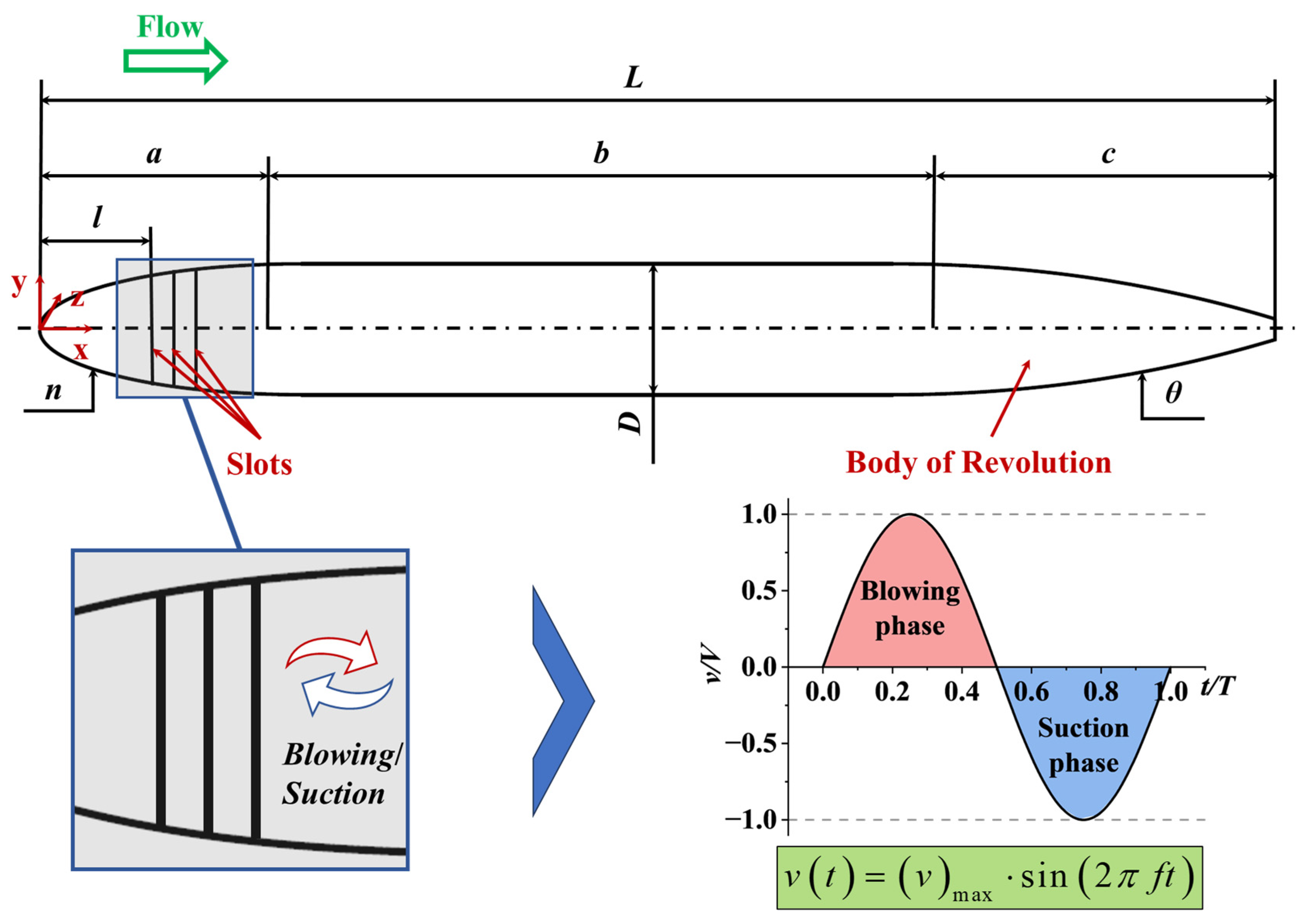
2.1. Body-of-Revolution Model

A sinusoidal periodic force produces good drag reduction for an underwater vehicle modeled as a body of revolution with a series of annular slots in the bow. In the present work, we use a model vehicle with a cylindrical shape for the midship; for the head and tail, we use Myring profiles, which have many successful applications in engineering [38]. The bow shape is described by a modified semielliptical radius distribution as:

$$r\left(x\right)={\displaystyle \frac{1}{2}}D\lceil 1-({\displaystyle \frac{x-a}{a}}{)}^2{\rceil }^{{\displaystyle \frac{1}{n}}}$$

(1)

The stern shape is defined by a cubic relationship as:

$$r\left(x\right)={\displaystyle \frac{1}{2}}D-\left({\displaystyle \frac{3D}{2c^2}}-{\displaystyle \frac{\mathrm{t}\mathrm{a}\mathrm{n}\theta }{c}}\right){\left(x-a-b\right)}^2+\left({\displaystyle \frac{D}{c^3}}-{\displaystyle \frac{\mathrm{t}\mathrm{a}\mathrm{n}\theta }{c^2}}\right){\left(x-a-b\right)}^3$$

(2)

Here, a, b, and c are the length of the bow, midship, and stern, respectively; D is the midship diameter; x is the axially projected distance from a point on the shape lines of the hull to the apex of the bow; r(x) is the radius of the body of revolution at point x; n is the index of the bow shape; and θ is the stern semi-angle. Larger values of n and θ result in a plumper body of revolution. The total length of the model is L. Three annular slots are provided: the distance between them is d, the width of each slot is w, and the distance of the first slot (the one nearest the bow) from the bow apex is l.

The model is shown in Figure 1. The blowing/suction wall-normal-phase velocity v is:

$$v\left(t\right)={\left(v\right)}_{\mathrm{m}\mathrm{a}\mathrm{x}}\cdot \mathrm{s}\mathrm{i}\mathrm{n}\left(2\pi ft\right)$$

(3)

where t is time and f is frequency (the reciprocal of the period T).

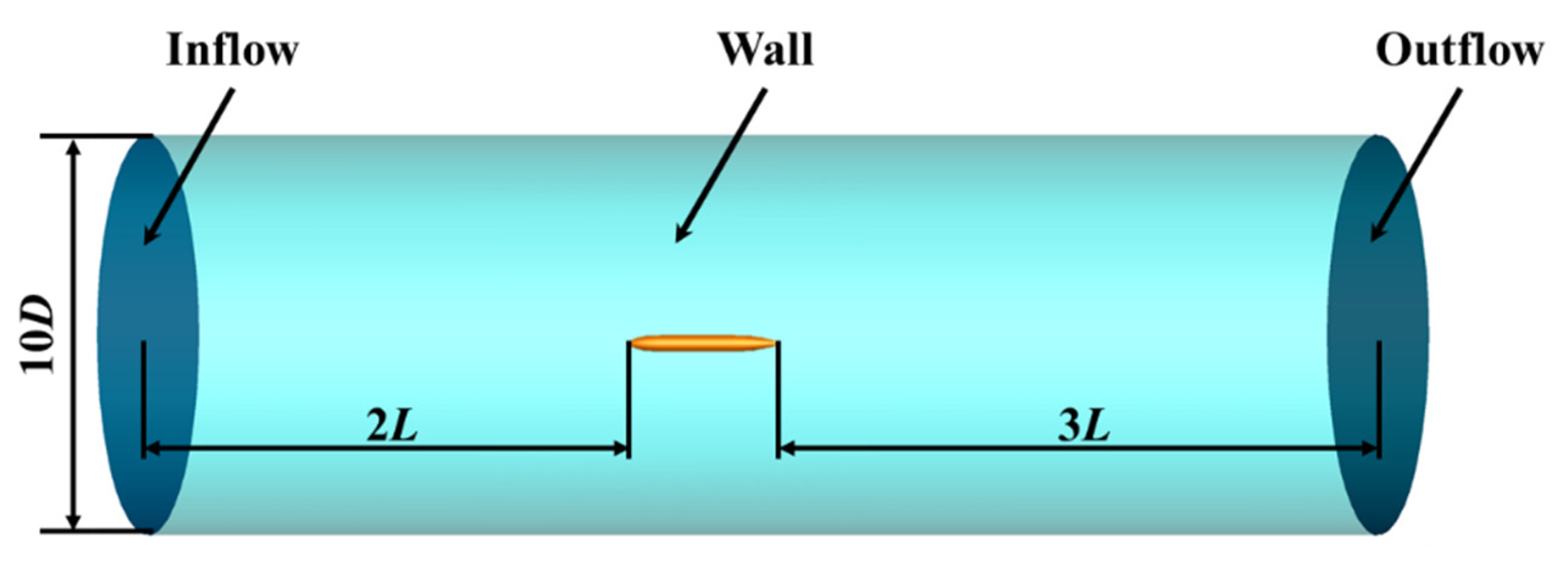
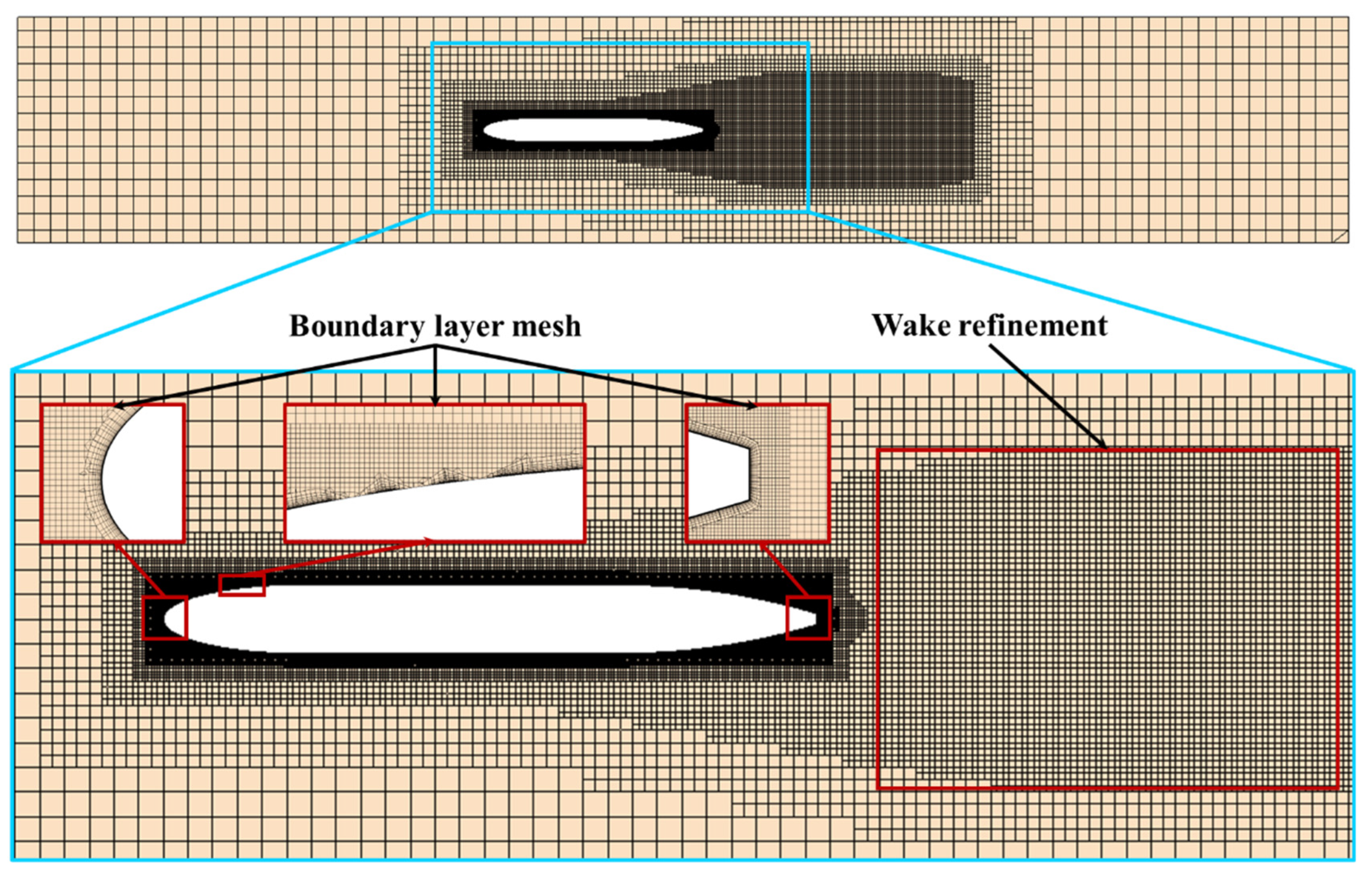
2.2. Numerical Method

Computational fluid dynamics (CFD) numerical simulations were performed using the commercial software STAR-CCM+. The implicit unsteady-flow simulation was based on the Reynolds-Averaged Navier–Stokes (RANS) equations and the shear-stress transport (SST) k-ω model. For boundary-layer flows, the k-ω model is superior both in its treatment of the viscous near-wall region, and in its accounting for the effects of streamwise pressure gradients. The k-ε model is incorporated into most commercial CFD codes, and it is generally regarded as being easy to use and computationally inexpensive when it is used in conjunction with wall functions [39]. SST k-ω utilizes the robustness of the k-ω model in the near-wall to capture the flow in the viscous bottom layer. And utilizing the k-ε model in the mainstream region can provide higher accuracy and reliability. Compared to other models, the SST k-ω model has better algorithmic accuracy and stability in the near-wall region, and it is highly accurate for the simulation of separated flow [40,41]. In accordance with the ITTC (International Towing Tank Conference) guidelines, time-step Δt should be smaller than 0.01 L/V if one or two equation turbulence models are used. An independent validation of the Δt was conducted in this study, and the results show that Δt is slightly larger than 0.01 L/V and has the same tendency and convergence characteristics as that of less than 0.01 L/V, and the instantaneous drag is slightly different from that of 0.01 L/V, which does not affect the conclusions of this study. Therefore, considering the overall computational cost and the data volume, the Δt of present numerical simulations is T/8 (0.0625 s). The instantaneous drag varied periodically under the influence of the periodic force. Its peak and trough values fluctuated over time within a certain range related to the amplitude and frequency. A termination criterion based on the monitored values was chosen and a convergence criterion was established using the asymptotic-limit method.

For hydrodynamic performance analysis, the model was considered to be submerged in a cylindrical fluid region surrounded by a virtual boundary large enough to develop the flow field fully, thus ensuring the efficient use of computational resources. As shown in Figure 2, the velocity-inlet boundary was located at 2 L upstream from the model; the flow velocity is denoted V. The pressure outlet condition was set at 3 L downstream from the model, and the outlet pressure was set to 0. The diameter of the computational domain was 10 D. The model was bounded by a no-slip wall. The velocity-inlet boundary condition was applied to the annular slots; the (control-fluid) inlet velocity was v(t) = (v)_max ∙ sin (2πft).

As shown in Figure 3, a structured mesh was used to discretize the computational domain. A fine mesh was used near the model, whereas a coarser mesh was chosen for areas away from the model where lower accuracy could be tolerated. In order to accurately capture the surrounding flow field of the body of revolution, mesh refinement was also performed in the wake area. The zoomed-in view in the figure shows the boundary layer and the localized encrypted meshes near the bow, stern, and slots. A boundary-layer mesh was deployed near the walls of the model; it was used to model the buffer sublayer with wall functions. In this study, 15 boundary layers were used. The thickness of the first layer of the mesh near the wall was $\Delta y={\displaystyle \frac{\mu y^{+}}{\rho u_{\tau }}}$, where μ is the hydrodynamic viscosity, ρ is the fluid density, and $u_{\tau }=\sqrt{{\tau }_w/\rho }$ is the wall-friction velocity. The nondimensional wall distance y⁺ = 3 was chosen to satisfy the SST k-ω modeling requirement [42] that it be <5. We considered the effects of variations in model velocities and dimensions, etc., on Re and mesh resolution and re-meshed for each case before numerical simulation.

2.3. Independence and Validation Study

To balance computational cost and simulation accuracy, mesh independence must be validated, and an appropriate mesh size determined. Numerical errors can be evaluated from the grid convergence index (GCI) [43]; this method has been widely used in numerical simulation [44,45]. In this study, multiple sets of meshes were created and computed based on a smooth body-of-revolution model.

Table 1. Details of the grid independence study.

(a) GCI Estimation of WSS
Mesh Size (q/Million Cells)	WSS (τw/Pa)	GCI (%)	Relative Errors (${\mathit{\delta }}_{{\mathit{\tau }}_{\mathit{\omega }}}$/%)
0.91	5.340	18.51	3.26
1.74	5.651	32.33	5.50
3.43	5.692	3.81	0.72
7.24	5.728	2.94	0.63
15.93	5.729	0.08	0.02
(b) GCI Estimation of Drag
Number of Meshes (q/Million Cells)	Drag (D0/N)	GCI (%)	Relative Errors (${\mathit{\delta }}_{{\mathit{D}}_{\mathbf{0}}}$/%)
0.91	18.409	22.05	3.91
1.74	19.246	25.24	4.35
3.43	19.291	1.23	0.23
7.24	19.356	1.57	0.34
15.93	19.299	1.28	0.30

presents the mesh size, wall-shear stress (WSS), drag (D₀), relative errors (δ), and GCI values. The variations in WSS and drag with the mesh quantity are shown in Figure 4, as is the asymptotic behavior of the GCI.

The calculated drag and WSS converged with increasing mesh size, and the relative error and GCI values decreased. At mesh sizes of 7.24 million and 15.93 million, the GCIs were not higher than 3% and all followed the mesh-convergence-index criterion [46]. A mesh solution with 7.24 million cells was chosen for subsequent analysis to ensure simulation accuracy and reduce computational costs.

In order to demonstrate that the simulation results are independent of the computational domain, we performed two more simulations with computational domain sizes of (4 L, 6 L) and (10 L, 15 L), and the simulation results are shown in

Table 2. Details of the computational domain independence study.

Computational Domain Size	WSS (τw/Pa)	Pressure Drag (DP0/N)	Frictional Drag (DF0/N)	Drag (D0/N)
(2 L,3 L)	5.728	1.243	18.112	19.356
(4 L, 6 L)	5.723	1.266	18.098	19.364
(10 L, 15 L)	5.722	1.262	18.094	19.357

. The simulation results show that the present computational domain size can ensure the simulation accuracy.

This study used the same simulation parameters as a published study by Stroh et al. of uniform-blowing drag reduction in flat-plate boundary layers [47]. The variation in flat-plate boundary-layer local surface-friction coefficients in the flow direction was obtained to verify that the current active control CFD models can produce convincing results. Figure 5a shows the flow-direction evolution of the surface-friction coefficient in the uncontrolled condition; the effect of control by uniform blowing is shown in Figure 5b. In the figure, the x-axis represents the flow-direction length of the flat-plate boundary layers, and the y-axis is the local surface-friction coefficient. It can be seen that the present study is in general agreement with the results of Stroh et al.

The SUBOFF model is a body of revolution with a total length of 4.356 m and a maximum diameter of 0.508 m. Its properties are well-known from tank and wind-tunnel tests, and it has been used to validate CFD simulations in many studies [48,49]. Figure 6 indicates that the simulated and measured total drags of the bare hull were in agreement: the total drag of SUBOFF increased gradually with the increase in velocity. According to

Table 3. Relative errors of numerical and experimental resistance values for SUBOFF.

Velocity (knots)	Experimental Results (DE/N)	Numerical Results (DN/N)	Relative Errors (δDt/%)
5.92	87.4	89.1	−1.95
10.00	242.2	232.5	4.00
11.84	332.9	317.9	4.51
13.92	451.5	429.1	4.96
16.00	576.9	553.3	4.09
17.99	697.0	685.9	1.59

, the maximum relative error for the model drag was 4.96%. In the table, D_E is the SUBOFF model tow tank result, D_N is the simulation result of this study, and δ_Dt is the relative error of the numerical simulation result. The numerical results verify the reliability and accuracy of CFD simulations.

3. Simulation Results

3.1. Adjustability and Stability Analysis

3.1.1. Adjustability Studies

In this study, we focus only on the effect of the slot area S, v, L, and V on the periodic force-reducing drag. To control for variables, the number of slots, L/D and a/D were held constant and d and l varied proportionally to exclude their effects, although they may indeed significantly affect periodic force drag reduction.

Table 4. Dimensions and velocities of various autonomous underwater vehicles.

Name	Dimension (m)	Velocity (m/s)
Hugin [2]	L: 6.90 m D: 0.75 m	3.0864
Remus 6000 [50]	L: 3.84 m D: 0.71 m	2.572
Remus M3V [51]	L: 0.91 m D: 0.124 m	5.144
Bluefin-21 [50]	L:4.93 m D: 0.533 m	2.572
Explorer [52]	L: 7.4 m D: 0.74 m	1.5
Autosub6000 [53]	L: 5.5 m D: 0.9 m	1.75
Sea-Whale [5]	L: 3 m D: 0.35 m	0.5

shows typical modern underwater-vehicle sizes and travel velocities for comparison.

S and v are related to L and V. The normalized periodic-forcing amplitude is denoted as A⁺ = v_max/V, and the relative slot size as w⁺ = w/L, the S = πDw. The relative flow rate is Q⁺ = A⁺ (w⁺)², which can be characterized in terms of A⁺ and w⁺. The control-variable method was adopted to discuss the drag-reduction effects of L, V, S, and v. Note that L and V characterize Re, whereas S and v characterize the instantaneous flow rate Q of the periodic force (Q = Sv). The model of the comparison group used in this study (represented by the subscript 0 in

Table 5. Numerical modeling cases for drag-fluctuation analysis.

Cases	L/L0	V/V0	S/S0	v/v0	A+/A+0	w+/w+0	Cases	L/L0	V/V0	S/S0	v/v0	A+/A+0	w+/w+0
1	1/2	1	1	1	1	4	10	1	1	1/4	1	1	1/4
2	√2/2	1	1	1	1	2	11	1	1	1/2	1	1	1/2
3	1	1	1	1	1	1	3	1	1	1	1	1	1
4	√2	1	1	1	1	1/2	12	1	1	2	1	1	2
5	2	1	1	1	1	1/4	13	1	1	4	1	1	4
6	1	1/4	1	1	4	1	14	1	1	1	1/4	1/4	1
7	1	1/2	1	1	2	1	15	1	1	1	1/2	1/2	1
3	1	1	1	1	1	1	3	1	1	1	1	1	1
8	1	2	1	1	1/2	1	16	1	1	1	2	2	1
9	1	4	1	1	1/4	1	17	1	1	1	4	4	1

) was a certain type of AUV profile, in which a, c, D, l, and L₀ are 700 mm, 1100 mm, 350 mm, 300 mm, and 3300 mm, respectively, V₀ is 2 m/s, S₀ is 5026 mm², v₀ is 2 m/s, f is 2 Hz, A⁺₀ is 1, and w⁺₀ is 0.0015. The bodies of revolution in all cases varied proportionally from the comparison group model. The scheme is shown in Table 5. In Cases 1–5, 6–9, 10–13, and 14–17, the variables L, V, S, and v, respectively, were varied separately, with the other three held constant. A⁺ and w⁺ are different in each case; A⁺/A⁺₀ and w⁺/w⁺₀ ranged from 1/4 to 4, respectively.

The simulation results in Figure 7a show that the variations in the average drag with L under the periodic force condition (case 1–5). As L/L₀ grow from 1/2 to 2, the frictional drag rapidly increases from 3.7 N to 59.8 N, while the pressure drag grows from −0.5 N to 3.63 N, and the drag-reduction rate decreases from 40.6% to 8.5%. Figure 7b presents the variations in the average drag with V (case 6–9). With the change in V/V₀ from 1/4 to 4, the friction drag increases rapidly to 215.2 N, while the pressure drag increases by 27.3 N, and the drag-reduction rate decreases from 119.1% to 3.9%. Figure 7c represents the variations in average drag with S (case 10–13). As S/S₀ changes from 1/4 to 4, the frictional drag and pressure drag produce a weak change, decreasing by 2.6 N and 3.9 N, respectively, and the drag-reduction rate is increased from 8.3% to 42.1%. Figure 7d illustrates the variations in the average drag with v (case 14–17). As v/v₀ grows from 1/4 to 4, the frictional drag does not produce a significant change, but the pressure drag decreases rapidly and the drag-reduction rate increases from 4.6% to 135.3%. The drag-reduction rate above can be expressed as $\overline{R}={\displaystyle \frac{D_0-\overline{D}}{D_0}}$, where D is the average drag on the periodic-force surface body of revolution.

The variations in L, S, V, and v signified the increase or decrease in w⁺ and A⁺. However, the effects of the four variables on the drag-reduction rate were not linear and differed in magnitude. Q had a stronger effect than Re, and the surface pressure pushed the model when S and v were higher than S₀ and v₀. In particular, the lowest pressure drag was -26.4 N with v increasing, and the maximum drag-reduction rate of total drag exceeded 135%.

3.1.2. Stability Studies

Periodic fluctuations in instantaneous drag that severely affect the stability of navigation control may be also related to L, V, S, and v; they are mainly influenced by pressure drag. Figure 8 presents the relationship between the fluctuations in pressure drag and the four variables. ΔD_P represents the pressure-drag amplitude (difference between the maximum and minimum values) in a single period. From the physical model, it is clear that in the limiting case where L, S, and v approach zero, the fluctuations in pressure drag caused by the periodic force will also disappear. As shown in Figure 8a,c,d, ΔD_P had an approximately linear relationship to L, S, and v, with straight-line fits passing through the origin. From Figure 8b, the relation between ΔD_P and V was complicated; for the convenience of the study, it was assumed to be a quadratic curve, which, according to the physical model, does not pass through the origin of the coordinate axes. The average slope of the three straight lines shown in Figure 8a,c,d was 44.2, and the relative errors were less than 10%. Therefore, to facilitate the study, the three lines were considered to have the same slope, and it was initially assumed that:

ΔD_P = (L/L₀)(S/S₀)(v/v₀)[K_α1(V/V₀)² + K_α2(V/V₀) + K_α3]

(4)

where K_α1, K_α2, and K_α3 are the fitting parameters.

In order to obtain a simple equation relating ΔD_P to L, V, S, and v (and thus quantitatively describe the instability induced by the periodic force during navigation), we simulated a large number of cases with periodic forcing. And based on the numerical simulation results, the values of each parameter shown in

Table 6. Parameters characterizing the pressure-drag fluctuation amplitude ΔD_P.

Parameter	Value
Kα1	−1.248
Kα2	8.784
Kα3	36.360

were obtained using the least-squares method.

In order to validate these results, 10 sets of cases with different L, V, S, and v were randomly set up for numerical simulation. As shown in

Table 7. Validation scheme for pressure-drag periodic-fluctuation equation.

L/L0	v/v0	V/V0	S/S0	Calculation Results (ΔDPc/N)	Simulation Results (ΔDPs/N)	Relative Errors $({\delta }_{{\Delta \mathit{D}}_{\mathit{P}}}$/%)
0.25	1	1	0.25	2.74	2.59	5.79
0.5	1	1	0.5	10.97	12.08	9.19
1	0.25	0.25	1	9.61	9.7	0.93
1	0.5	0.5	1	20.21	21	3.76
1	2	2	1	97.87	106.04	7.70
1	4	2	1	103.22	112.57	8.31
1	2	4	1	195.75	180.79	8.27
2	1	1	2	175.5	188.46	6.88
2	1	1	4	351	334.7	4.87
4	1	1	4	702	652.01	7.67

, the relative errors between the numerical results and the results from Equation (4) were all within 10%, indicating that the equation can roughly describe the relationship between the fluctuation of pressure drag and the four variables in this study. In the table, ΔD_Pc denotes the calculation results from Equation (4), and ΔD_Ps denotes the results obtained by numerical simulations.

Because S = πDw, v and w can be expressed as A⁺ V and w⁺L, respectively. If w⁺/w₀⁺ = A⁺/A₀⁺ = 1, Equation (4) can be simplified to:

ΔD_P = (L/L₀)³ [K_α1(V/V₀)³ + K_α2(V/V₀)² + K_α3(V/V₀)]

(5)

Figure 9 shows that ΔD_P increased as L/L₀ and V/V₀ increased. When L/L₀ reached 2, ΔD_P increased especially rapidly. Therefore, under the same control parameters, a smaller, slower underwater vehicle has better stability, and an underwater vehicle with a size less than 2L₀ is more stable than a larger vehicle with the same velocity.

Placing multiple tandem slots in a dispersed row and executing periodic blowing and suction in sequence ensures that at least one set of slots is in the blowing phase at any given moment. This can transform unstable control into a relatively stable condition, as shown in Figure 10.

3.2. Surface-Pressure and Velocity Analysis

3.2.1. Surface-Pressure Analysis

Periodic forcing changes the turbulent structure of the surface. Figure 11 shows the surface boundary-layer pressure coefficients of Cases 3, 4, 8, 12, and 16 with and without periodic forcing. The pressure coefficient in the figure is $C_p=f\left(\overline{y}\right)={\displaystyle \frac{P-P_{\mathrm{\infty }}}{0.5\rho V^2}}$, where P is the surface pressure and P_∞ is the far-field water pressure. Blowing increased the model surface pressure, and suction decreased it. Without control, the surface-pressure distribution was approximately the same for the same velocity. However, because of Bernoulli’s principle, there was a large difference in the surface-pressure distribution for models of the same size at different velocities. As velocity increased, the dynamic pressure on the surface rose rapidly and the pressure coefficient fell. As in Figure 11, the pressure distributions in the boundary layer under periodic forcing were almost the same for different L, S, and v. However, with changes in V, the pressure distribution became complicated.

Figure 12 shows the distributions of relative pressure coefficients on the model surfaces when periodic blowing and suction were applied. The superscript * on a pressure coefficient means “uncontrolled;” $\overline{y}$ = y/δ and $\overline{x}$ = x/δ are dimensionless representations of the normal and flow distances from the model surface, respectively; x and y are the flow and normal distance; and δ is the thickness of the model boundary layer.

Figure 12a shows the downstream relative pressure-coefficient distribution of slots during blowing and suction. Consistent with Figure 11, the surface pressure increased during blowing and decreased during suction. The relative pressure gradient was directly related to w⁺ and A⁺. Figure 12b shows that the pressure gradients of Cases 4 and 8 were smaller than that of Case 3; those of Cases 12 and 16 were significantly larger than that of Case 3. The effects of L and V on the pressure gradient were roughly the same, but the surface pressure of Case 8 was lower. The same is demonstrated in Figure 7a,b and Figure 11. On the other hand, the pressure gradient of Case 16 was significantly larger than that of Case 12, in agreement with the conclusions from Figure 7c,d that v exerts a greater influence on the surface-pressure distribution relative to S.

Under periodic forcing, there were significant pressure gradients in both the x and y directions. Clockwise vortices were generated on the model surface and developed downstream, as shown in Figure 13. The vortex scales were clearly affected by the relative pressure gradient; a decrease in A⁺ and w⁺ decreased the relative pressure gradient and vortex scale, and conversely, an increase in A⁺ and w⁺ increased the vortex scale. Consistent with the results shown in Figure 7, the large-scale vortices caused by larger A⁺ and w⁺ could effectively reduce the average pressure drag on the model surface.

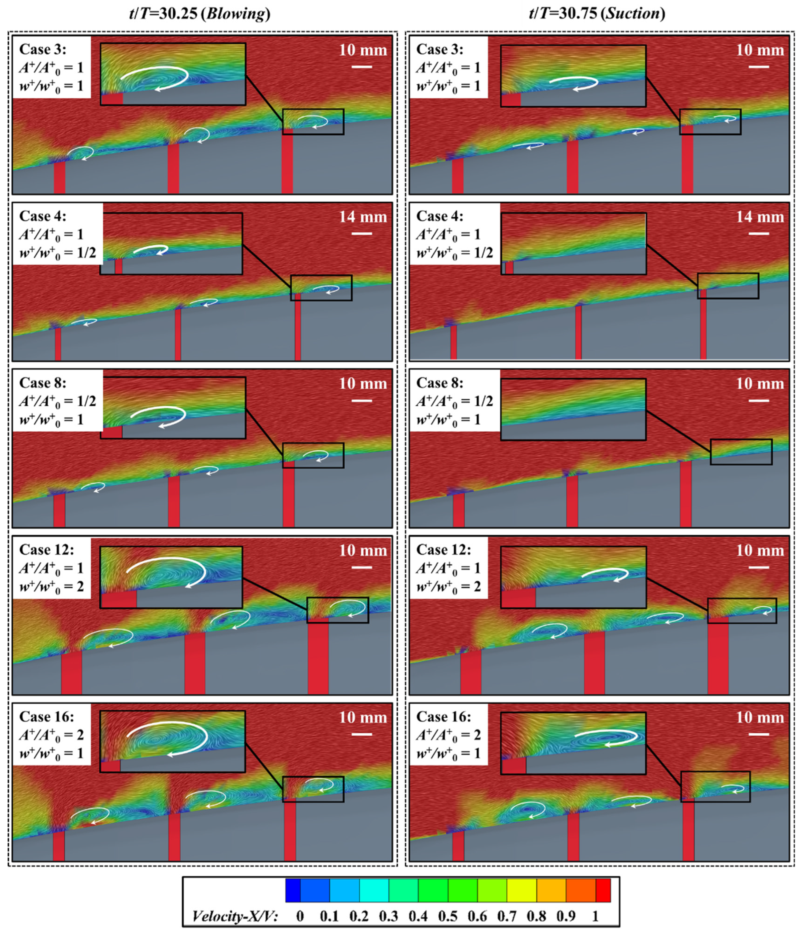
3.2.2. Surface-Velocity Analysis

Figure 14 exhibits the relative-velocity contours of the model surfaces under periodic forcing. Compared to Case 3, the surface velocities decreased in Cases 4 and 8, and increased in Cases 12 and 16. Like the surface-vortex scale, the boundary-layer structure was affected by A⁺ and w⁺. Larger A⁺ and w⁺ values were correlated with larger boundary-layer thicknesses and smaller velocity gradients $\partial \stackrel{\mathrm{-}}{V}/\partial y$, which reduced the frictional drag. In addition, the blown fluid played a blocking role and formed a slow-flow zone in front of the annular slots.

The turbulent-kinetic-energy contours of the periodic jet surface are shown in Figure 15. Higher A⁺ and w⁺ dramatically increased the turbulent kinetic energy while reducing the drag. Periodic forcing increased fluid-transport strength near the wall surface and thus the turbulent kinetic energy; the pulsation velocity and Reynolds shear stress were elevated accordingly. This shows that suppression of turbulence near the wall is crucial for enhancing the drag-reduction rate. Good results can be achieved not only by combining the use of a periodic force with compliant wall and riblet surfaces to reduce the turbulence intensity but also by selecting appropriate values of A⁺ and w⁺.

4. Discussion

We used numerical simulations to investigate the adjustability and stability of the periodic-forcing drag-reduction technique. Periodic blowing and suction reduce drag because the fluid upstream from the slots is blocked during blowing, and a low-pressure zone is formed downstream from the slots; thus, vortices develop downstream, reducing the pressure drag. On the other hand, the blown high-velocity fluid accelerates the viscous fluid near the wall, which thickens the boundary layer, reduces the velocity gradient, and lowers the frictional drag. By contrast, during suction, the vortices decrease or even disappear, and the suction fluid further reduces the velocity of the boundary-layer fluid downstream from the slots, increasing the pressure difference and friction drag.

The drag reduction and periodic fluctuations of instantaneous drag may be related to L, V, S, and v. This was investigated in Cases 1–17. Changes in L, S, V, and v in these cases signified changes in w⁺ and A⁺, respectively. The drag-reduction rate increased and decreased with the growth and decline of w⁺ and A⁺. The effects of the four parameters L, V, S, and v on the drag-reduction rate were not linear, and there were differences in their effects on the drag. Figure 7a,b shows that as L and V were proportionally increased, leading to a proportional decrease in w⁺ and A⁺, the drag-reduction rate gradually decreased. L/L₀ grows from 1/2 to 2, the total drag increases from 3.2 N to 63.4 N, and the drag-reduction rate decreases from 40.7% to 8.5%; V/V₀ grows from 1/2 to 2, the total drag increases from 2.8 N to 62.6 N, and the drag-reduction rate decreases from 47.5% to 10.1%. Therefore, we suggest that, in keeping Q constant, L and V have similar effects on the drag-reduction rate. Figure 7c,d illustrate that, in keeping Re constant, there was a large difference in the effect of S and v on drag. The pressure drag decreased more significantly (by 28.2 N) when v increased across the range than when S did; moreover, as v increased, the friction drag increased again after a small decrease. With the proportional rise of S and v, w⁺ and A⁺ also rose. Under the control of S, the drag-reduction rate gradually increased, but the rise gradually decreased as a result of pressure drag and friction drag. Under v control, the drag-reduction rate rose sharply; this was caused by the large reduction in pressure drag.

As Figure 8 shows, ΔD_P had an approximately linear relationship with L, S, and v, and an approximately quadratic relationship with V. In this study, a simple equation for ΔD_P as a function of L, V, S, and v has been proposed to describe the periodic fluctuations of pressure drag under the influence of periodic forcing; such an equation has not been proposed in previous studies. It predicts that under the same control parameters and free flow velocity, underwater vehicles with sizes smaller than 2L₀ will achieve more stable navigation.

S and v boosting controls the flow in different ways. The expansion of S does not increase the blowing velocity. It has less effect on the pressure distribution near the slots than does v boosting, as shown in Figure 12b, and more effect on the fluid velocity on the near-wall of the boundary layer. Excessively large values of v may disrupt the structure of the boundary layer downstream from the slots, resulting in an increase in frictional drag (Figure 14). Therefore, increasing S reduces the pressure and friction drag; increasing v reduces the pressure drag, but too large a v causes a rise in friction drag.

Higher values of w⁺ and A⁺ increase the scale of vortices caused by the periodic force as well as the thickness of the boundary layer. This reduces the pressure and frictional drag, as can be seen by analyzing the surface pressure and velocity. However, the distribution of surface turbulent kinetic energy (Figure 15) shows that high w⁺ and A⁺ dramatically increase the pulsation velocity and Reynolds shear stress near the wall while reducing the drag. The compliant wall suppresses fluid-pressure pulsations and absorbs turbulent energy, and the riblet also suppresses high-frequency fluctuations and reduces Reynolds stresses. Some studies have indicated that specific compliant wall and surface riblet designs provide better drag reduction at low flow velocities [54,55]. Similarly, in this study, periodic forcing produced better stability at low Re for the same w⁺ and A⁺. Possibly, better drag reduction could be obtained by using an active–passive drag-reduction design for low-speed underwater vehicles that combines periodic forcing with a compliant wall or riblet surfaces. However, the selection of the appropriate w⁺ and A⁺ is equally critical.

Periodic forcing has been explored for many flow control applications in aerodynamics; it can effectively improve the aerodynamic performance of aircraft [56,57,58]. Previous studies have found that periodic forcing moves the high-momentum fluid downstream along the airfoil suction surface, suppresses flow separation, and draws in high-velocity fluid at the front edge of the airfoil during the suction phase; this reduces the airfoil suction surface pressure and improves the lift-to-drag ratio [57,59]. For supersonic or hypersonic aircraft, shock-wave drag accounts for a large portion of the total drag; periodic forcing can reduce drag by pushing the shock wave away [60].

Because seawater is significantly denser and more viscous than air, the velocity of an underwater vehicle is much lower than that of an aircraft; therefore, the frictional drag accounts for a higher percentage of the total drag, and the flow field structure is likely to be more stable. On the other hand, fluid separation is dominated by inertial effects in underwater flow, whereas pressure gradients are more important in aerial flow. Therefore, the main contribution of periodic forcing to the hydrodynamic performance of underwater vehicles lies in the reduction in the velocity gradient along the flow direction, which lessens surface-friction drag [61]. Because of the density and high pressure of seawater, periodic forcing on an underwater vehicle consumes more energy than on an airfoil, which has discouraged its use. Nevertheless, there are enough similarities between underwater and aeronautical effects of periodic forcing, including acceleration of surface fluid, a suction-induced pressure drop near the slots, and suppression of flow separation by high-velocity fluid, to warrant further research.

Drag reduction is not the only advantage periodic forcing offers to underwater vehicles. For example, it may be used to enhance the hydrodynamic performance of underwater gliders and other lift-driven underwater vehicles, much as it increases lift in aeronautical vehicles. Other characteristics of periodic forcing, such as low noise and the ability to create minimal flow obstacles, make it ideal for low-speed underwater propulsion and steering control. Periodic blowing and suction are similar to the propulsion mechanism of marine organisms such as jellyfish and squid: when these animals move, the boundary layer separates and rolls up as the fluid is ejected from the cavity, forming a vortex ring for efficient propulsion [62]. Blowing and suction are also suitable for steering applications because the periodic-force actuator is compact and small enough to be mounted completely inside the vehicle, generating negligible additional drag [63].

Although the qualitative and quantitative results given in this study are from numerical simulations of a specific body-of-revolution model with particular sizes and speeds, these parameters fall within the range of those widely used in current AUVs [34,35,36,37]. The methodology and some of the results of this paper can be extended to larger or smaller sizes and speeds as well as to other columnar structures that are not bodies of revolution (e.g., large submarines or manned submersibles), because the periodic control creates vortices and moves them downstream, independently of the model line shape. This has been demonstrated by previous studies of active flow-control drag reduction for a variety of models and control parameters [17,20,21,33].

However, there are some limitations to this study. In general, passive drag-reduction methods rely on design or material properties to reduce drag without additional energy input but are only applicable to a particular operating condition [13]. Active drag reduction, on the other hand, uses an external energy or material supply to achieve fluid control; this is much more adaptable but is only truly effective if the drag reduction exceeds the input energy required to achieve it [64]. A deeper and more comprehensive quantitative study of the adjustability of periodic forcing to drag reduction requires further investigation of the energy input and saving rate required by periodic blowing and suction.

In summary, the application of periodic forcing to an underwater vehicle can effectively reduce the surface drag; the optimal drag-reduction effect is obtained by a reasonable choice of control parameters for a given velocity.

5. Conclusions

This study has investigated the adaptation and stability of local periodic forcing in incompressible fluids around a specific body of revolution. In particular, the drag-reducing effect of periodic blowing and suction through a series of tandem annular slots was considered. The following conclusions were obtained:

(1)

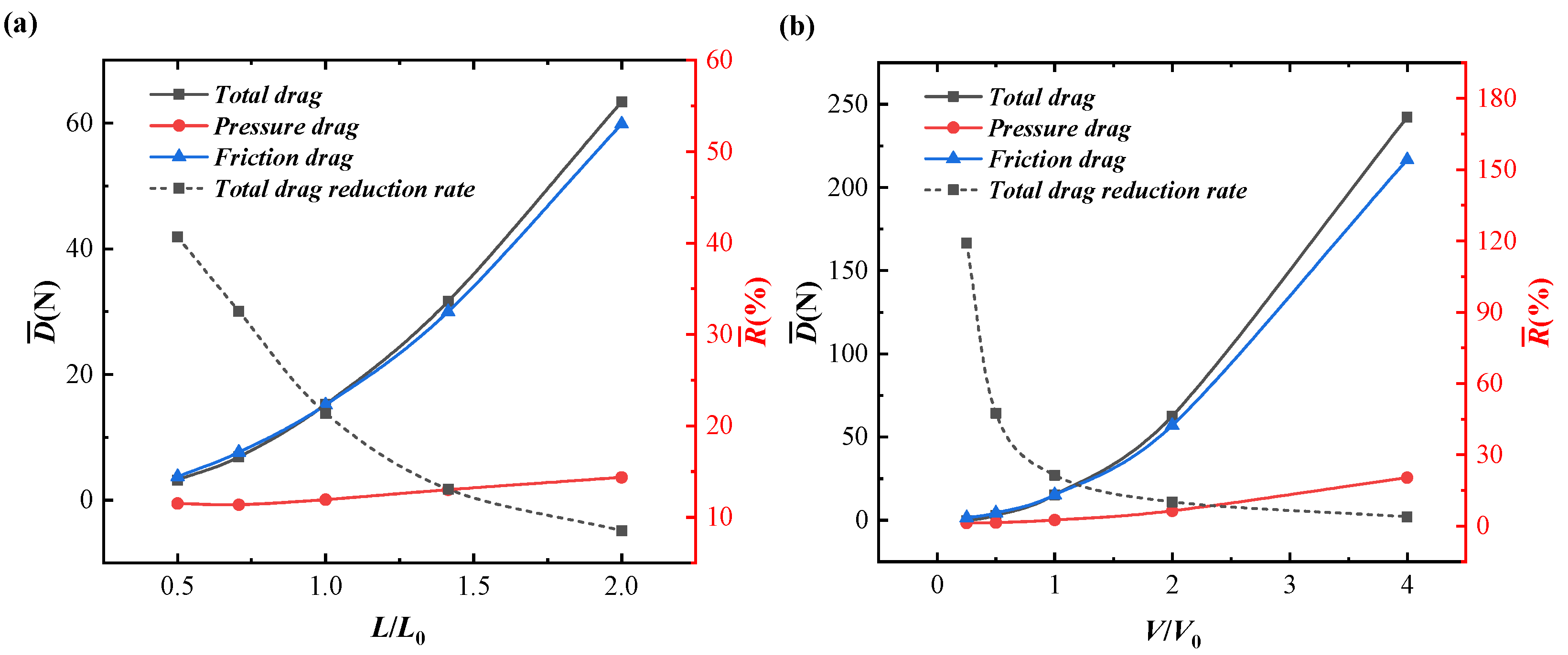
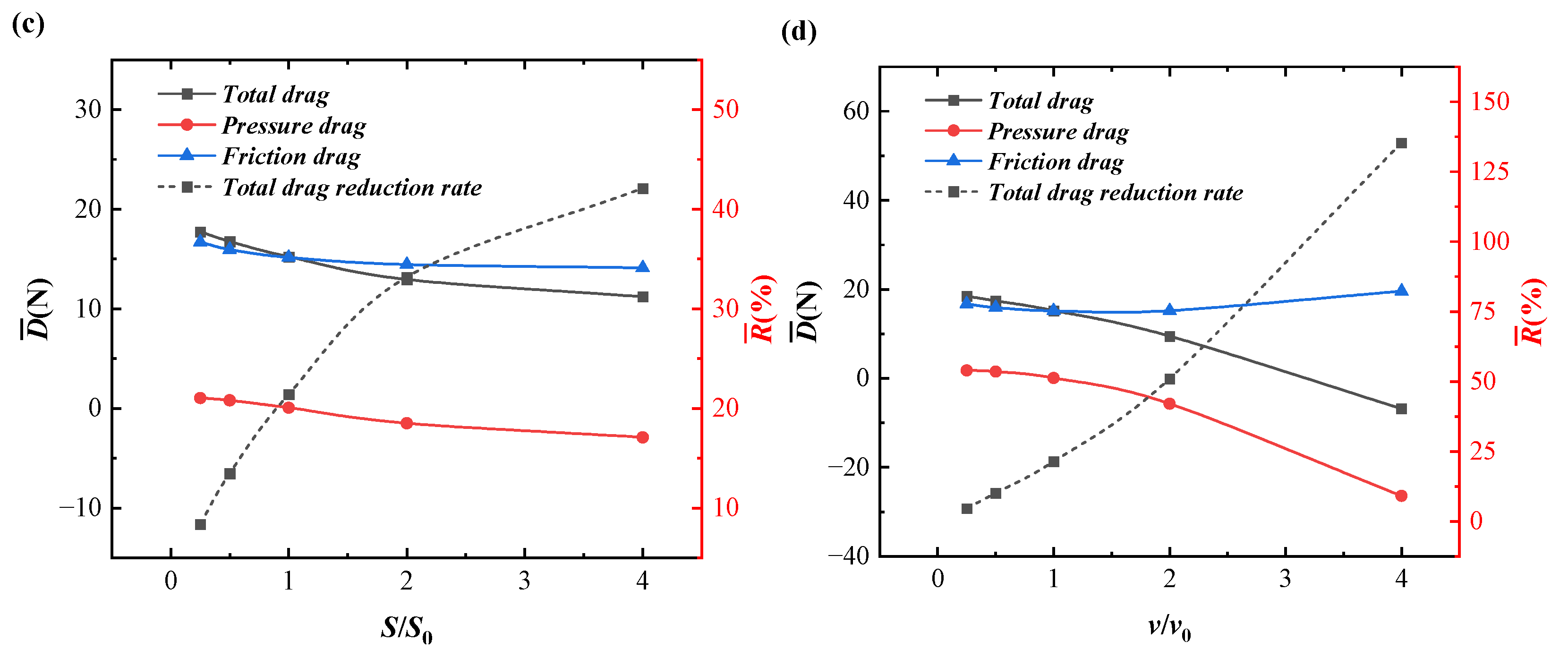
The drag-reduction rate increases with w⁺ and A⁺. The body variables (L, V, S, and v) differ in their effect on the drag-reduction rate, with v having a stronger effect than S. As v increases, the surface pressure pushes the model vehicle; the lowest pressure drag is −26.4 N, and the maximum drag-reduction rate of total drag exceeded 135%.

(2)

S and v enhance the control flow Q in different ways. The expansion of S accelerates the boundary layer near-wall fluid and further blocks the fluid upstream from the slots; to a certain extent, this expands the low-pressure region downstream from the slots. Thus, the pressure and frictional drag are reduced. The maximum drag-reduction rate is 42.1%. Excessive v exacerbates the blocking effect on the fluid upstream from the slots, which greatly increases the pressure gradient downstream from them and also destroys the downstream boundary-layer structure. This results in a substantial pressure-drag decrease of 27.7 N but also in a slight increase in frictional drag, with a frictional-drag-reduction rate of −8.5%.

(3)

Under the same control parameters, underwater vehicles with small sizes and low speeds are more stable. For a given speed, the navigational-stability benefit is greater for vehicles with a size less than 2L₀.

(4)

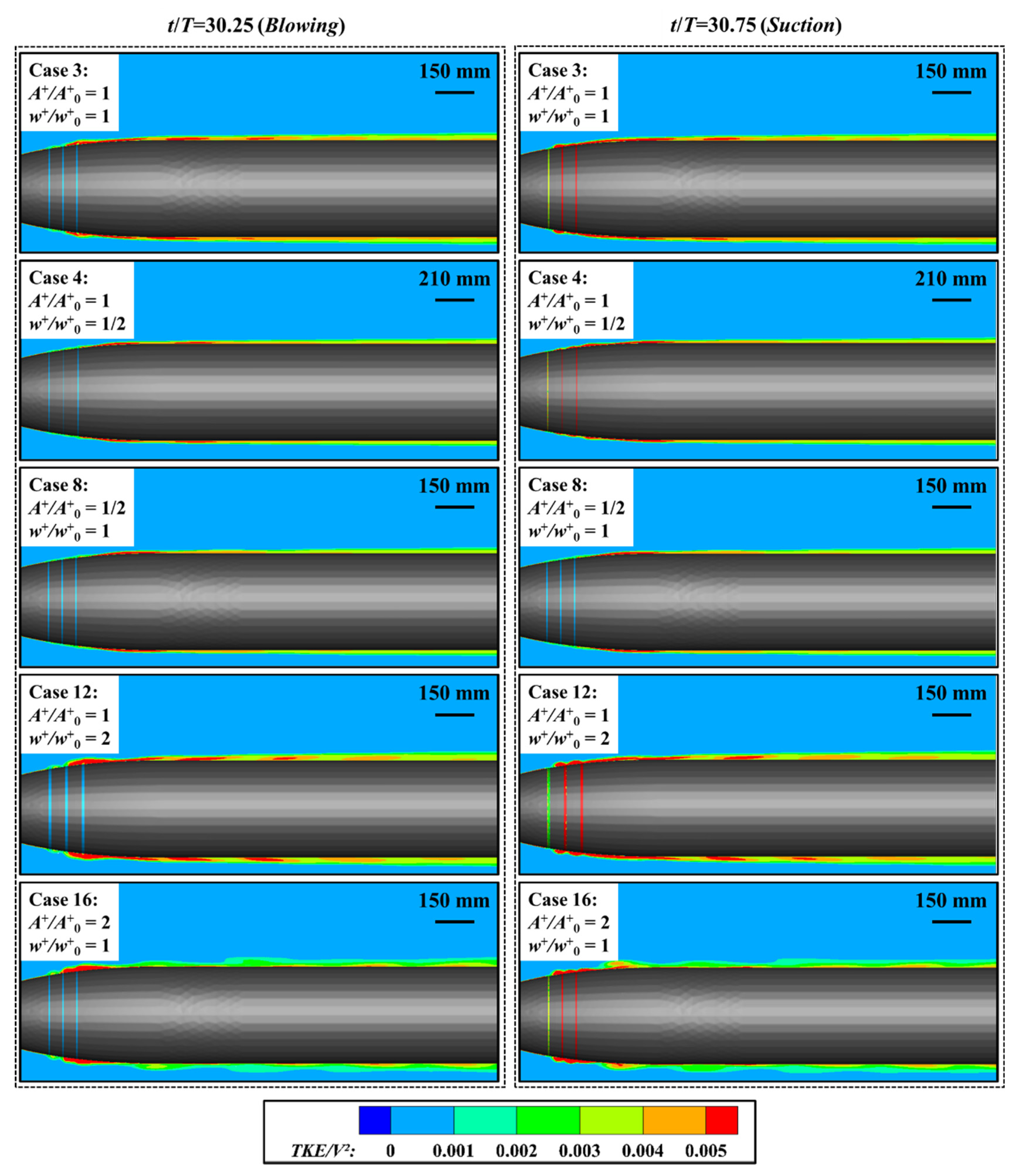
Analyzing the surface turbulent kinetic energy reveals that high w⁺ and A⁺ drastically increase the pulsation velocity and Reynolds shear stress near the wall while greatly reducing the drag. Therefore, a specific-size body of revolution with reasonably set control parameters (w⁺ and A⁺) and an appropriate velocity (Re) will achieve optimal drag reduction.

The model described in this paper can provide a new solution to the problem of surface-drag reduction and enhance the stability of underwater vehicles.

References

1. Zhang, B.; Ji, D.; Liu, S.; Zhu, X.; Xu, W. Autonomous underwater vehicle navigation: A review. Ocean Eng. 2023, 273, 113861. [Google Scholar] [CrossRef]
2. Zwolak, K.; Wigley, R.; Bohan, A.; Zarayskaya, Y.; Bazhenova, E.; Dorshow, W.; Sumiyoshi, M.; Sattiabaruth, S.; Roperez, J.; Proctor, A. The autonomous underwater vehicle integrated with the unmanned surface vessel mapping the Southern Ionian Sea. The Winning Technology Solution of the Shell Ocean Discovery XPRIZE. Remote Sens. 2020, 12, 1344. [Google Scholar] [CrossRef]
3. Sahoo, A.; Dwivedy, S.K.; Robi, P. Advancements in the field of autonomous underwater vehicle. Ocean Eng. 2019, 181, 145–160. [Google Scholar] [CrossRef]
4. Fiester, C.; Gomez-Ibanez, D.; Grund, M.; Purcell, M.; Jaffre, F.; Forrester, N.; Austin, T.; Stokey, R. A modular, compact, and efficient next generation remus 600 auv. In Proceedings of the OCEANS 2019-Marseille, Marseille, France, 17–20 June 2019; pp. 1–6. [Google Scholar]
5. Qiao, J.; Yu, J.; Huang, Y.; Cui, J.; Wang, B.; Wang, Z. Sea-Whale Series AUV-Extending the range to 4000 kilometers. In Proceedings of the OCEANS 2022, Hampton Roads, Virtual, 17–20 October 2022; pp. 1–5. [Google Scholar]
6. Cui, Z.; Li, L.; Wang, Y.; Zhong, Z.; Li, J. Review of research and control technology of underwater bionic robots. Intell. Mar. Technol. Syst. 2023, 1, 7. [Google Scholar] [CrossRef]
7. Liang, J.; Feng, J.-C.; Zhang, S.; Cai, Y.; Yang, Z.; Ni, T.; Yang, H.-Y. Role of deep-sea equipment in promoting the forefront of studies on life in extreme environments. Iscience 2021, 24, 103299. [Google Scholar] [CrossRef]
8. Abdulbari, H.A.; Yunus, R.; Abdurahman, N.; Charles, A. Going against the flow—A review of non-additive means of drag reduction. J. Ind. Eng. Chem. 2013, 19, 27–36. [Google Scholar] [CrossRef]
9. Kumar, S.; Pandey, K.M.; Sharma, K.K. Advances in drag-reduction methods related with boundary layer control–A review. Mater. Today Proc. 2021, 45, 6694–6701. [Google Scholar] [CrossRef]
10. Liu, G.; Yuan, Z.; Qiu, Z.; Feng, S.; Xie, Y.; Leng, D.; Tian, X. A brief review of bio-inspired surface technology and application toward underwater drag reduction. Ocean Eng. 2020, 199, 106962. [Google Scholar] [CrossRef]
11. Tian, G.; Fan, D.; Feng, X.; Zhou, H. Thriving artificial underwater drag-reduction materials inspired from aquatic animals: Progresses and challenges. RSC Adv. 2021, 11, 3399–3428. [Google Scholar] [CrossRef]
12. Perlin, M.; Dowling, D.R.; Ceccio, S.L. Freeman scholar review: Passive and active skin-friction drag reduction in turbulent boundary layers. J. Fluids Eng. 2016, 138, 091104. [Google Scholar] [CrossRef]
13. Zhang, L.; Shan, X.; Xie, T. Active control for wall drag reduction: Methods, mechanisms and performance. IEEE Access 2020, 8, 7039–7057. [Google Scholar] [CrossRef]
14. Meng, L.; Yang, L.; Su, T.C.; Gu, H. Study on the influence of porous material on underwater vehicle’s hydrodynamic characteristics. Ocean Eng. 2019, 191, 106528. [Google Scholar] [CrossRef]
15. Panda, J.P.; Warrior, H.V. Numerical Studies on Drag Reduction of an Axisymmetric Body of Revolution with Antiturbulence Surface. J. Offshore Mech. Arct. Eng. 2021, 143, 064501. [Google Scholar] [CrossRef]
16. Panda, J.P.; Warrior, H.V. Mechanics of drag reduction of an axisymmetric body of revolution with shallow dimples. Proc. Inst. Mech. Eng. Part M J. Eng. Marit. Environ. 2023, 237, 227–237. [Google Scholar] [CrossRef]
17. Che, Z.-X.; Huang, S.; Li, Z.-W.; Chen, Z.-W. Aerodynamic drag reduction of high-speed maglev train based on air blowing/suction. J. Wind. Eng. Ind. Aerodyn. 2023, 233, 105321. [Google Scholar] [CrossRef]
18. Posa, A.; Balaras, E. A numerical investigation of the wake of an axisymmetric body with appendages. J. Fluid Mech. 2016, 792, 470–498. [Google Scholar] [CrossRef]
19. Posa, A.; Balaras, E. A numerical investigation about the effects of Reynolds number on the flow around an appended axisymmetric body of revolution. J. Fluid Mech. 2020, 884, A41. [Google Scholar] [CrossRef]
20. Kametani, Y.; Fukagata, K.; Orlu, R.; Schlatter, P. Effect of uniform blowing/suction in a turbulent boundary layer at moderate Reynolds number. Int. J. Heat Fluid Flow 2015, 55, 132–142. [Google Scholar] [CrossRef]
21. Noguchi, D.; Fukagata, K.; Tokugawa, N. Friction drag reduction of a spatially developing boundary layer using a combined uniform suction and blowing. J. Fluid Sci. Technol. 2016, 11, JFST0004. [Google Scholar] [CrossRef]
22. Ma, R.; Gao, Z.-H.; Lu, L.-S.; Chen, S.-S. Skin-friction drag reduction by local porous uniform blowing in spatially developing compressible turbulent boundary layers. Phys. Fluids 2022, 34, 125130. [Google Scholar] [CrossRef]
23. Abbas, A.; Bugeda, G.; Ferrer, E.; Fu, S.; Periaux, J.; Pons-Prats, J.; Valero, E.; Zheng, Y. Drag reduction via turbulent boundary layer flow control. Sci. China Technol. Sci. 2017, 60, 1281–1290. [Google Scholar] [CrossRef]
24. Murugan, T.; Deyashi, M.; Dey, S.; Rana, S.C.; Chatterjee, P. Recent Developments on Synthetic Jets. Def. Sci. J. 2016, 66, 489–498. [Google Scholar] [CrossRef]
25. Ja’fari, M.; Shojae, F.J.; Jaworski, A.J. Synthetic jet actuators: Overview and applications. Int. J. Thermofluids 2023, 20, 100438. [Google Scholar] [CrossRef]
26. Park, S.; Lee, I.; Sung, H.J. Effect of local forcing on a turbulent boundary layer. Exp. Fluids 2001, 31, 384–393. [Google Scholar] [CrossRef]
27. Boiko, A.V.; Kornilov, V.I. Effect of periodic blowing/suction through sequentially located annular slots on the turbulent boundary layer on a body of revolution. Thermophys. Aeromechanics 2008, 15, 11–27. [Google Scholar] [CrossRef]
28. Kornilov, V.I.; Boiko, A.V. Periodic forcing of the turbulent boundary layer on a body of revolution. AIAA J. 2008, 46, 653–663. [Google Scholar] [CrossRef]
29. Kornilov, V.I.; Boiko, A.V. Advances and challenges in periodic forcing of the turbulent boundary layer on a body of revolution. Prog. Aerosp. Sci. 2018, 98, 57–73. [Google Scholar] [CrossRef]
30. Yang, R.; Luo, Z.; Xia, Z.; Wang, L.; Zhou, Y. Numerical study of plasma synthetic jet control on hypersonic missile. ACTA Aeronaut. Astronaut. Sin. 2016, 37, 1722–1732. [Google Scholar]
31. Gil, P. Bluff Body Drag Control using Synthetic Jet. J. Appl. Fluid Mech. 2019, 12, 293–302. [Google Scholar] [CrossRef]
32. Xie, F.; Perez-Munoz, J.D.; Qin, N.; Ricco, P. Drag reduction in wall-bounded turbulence by synthetic jet sheets. J. Fluid Mech. 2022, 941, A63. [Google Scholar] [CrossRef]
33. Li, H.; Yu, J.; Chen, Z.; Ren, K. Numerical research on drag-reduction characteristics of a body of revolution based on periodic forcing. Ocean Eng. 2023, 280, 114909. [Google Scholar] [CrossRef]
34. Fletcher, B. UUV master plan: A vision for navy UUV development. In Proceedings of the OCEANS 2000 MTS/IEEE Conference and Exhibition. Conference Proceedings (Cat. No. 00CH37158), Providence, RI, USA, 11–14 September 2000; pp. 65–71. [Google Scholar]
35. Yu-Ru, X. Expectation of the Development in the Technology on Ocean Space Intelligent Unmanned Vehicles. Chin. J. Ship Res. 2006, 1, 1–4. [Google Scholar]
36. Mondal, K.; Banerjee, T.; Panja, A. Autonomous underwater vehicles: Recent developments and future prospects. Int. J. Res. Appl. Sci. Eng. Technol. 2019, 7, 215–222. [Google Scholar] [CrossRef]
37. Furlong, M.E.; McPhail, S.D.; Stevenson, P. A Concept Design for an Ultra-Long-Range Survey Class AUV; IEEE: Piscataway, NI, USA, 2007. [Google Scholar]
38. Hang Hou, Y.; Liang, X.; Mu, X.Y. AUV hull lines optimization with uncertainty parameters based on six sigma reliability design. Int. J. Nav. Arch. Ocean Eng. 2018, 10, 499–507. [Google Scholar]
39. Pope, S.B. Turbulent Flows; Cambridge University Press: Cambridge, UK, 2000. [Google Scholar]
40. Catalano, P.; Amato, M. An evaluation of RANS turbulence modelling for aerodynamic applications. Aerosp. Technol. 2003, 7, 493–509. [Google Scholar] [CrossRef]
41. Mohanarangam, K.; Cheung, S.; Tu, J.Y.; Chen, L. Numerical simulation of micro-bubble drag reduction using population balance model. Ocean Eng. 2009, 36, 863–872. [Google Scholar] [CrossRef]
42. Li, F.; Zhao, G.; Liu, W. Research on drag reduction performance of turbulent boundary layer on bionic jet surface. Proc. Inst. Mech. Eng. Part M J. Eng. Marit. Environ. 2016, 231, 258–270. [Google Scholar] [CrossRef]
43. Roache, P.J. Quantification of uncertainty in computational fluid dynamics. Annu. Rev. Fluid Mech. 1997, 29, 123–160. [Google Scholar] [CrossRef]
44. Da Silva, F.D.; Tancredi, T.P.; Silva, E. Corrections for the drag on submarines due to the blockage effect. Ocean Eng. 2023, 275, 114150. [Google Scholar] [CrossRef]
45. Liu, J.; Wang, M.; Yu, F.; Gao, S.; Yan, T.; He, B. Numerical study on the hull–propeller interaction of autonomous underwater vehicle. Ocean Eng. 2023, 271, 113777. [Google Scholar] [CrossRef]
46. Manna, P.; Dharavath, M.; Sinha, P.K.; Chakraborty, D. Optimization of a flight-worthy scramjet combustor through CFD. Aerosp. Sci. Technol. 2013, 27, 138–146. [Google Scholar] [CrossRef]
47. Stroh, A.; Hasegawa, Y.; Schlatter, P.; Frohnapfel, B. Global effect of local skin friction drag reduction in spatially developing turbulent boundary layer. J. Fluid Mech. 2016, 805, 303–321. [Google Scholar] [CrossRef]
48. Liu, H.L.; Huang, T.T. Summary of DARPA Suboff Experimental Program Data. Summ. Darpa Suboff Exp. Progr. Data 1998. [Google Scholar]
49. Groves, N.C.; Huang, T.T.; Chang, M.S. Geometric Characteristics of DARPA (Defense Advanced Research Projects Agency) SUBOFF Models (DTRC Model Numbers 5470 and 5471). Geom. Charact. Darpa Suboff Models 1989. [Google Scholar]
50. Guo, Z.; Hong, M.; Shi, J.; Zhang, Y.; Qian, L.; Li, H. Risk assessment of unmanned underwater platforms in the South China Sea marine environment based on two-dimensional density-weighted operator and cloud barycentric Bayesian combination. Ocean Eng. 2023, 283, 115184. [Google Scholar] [CrossRef]
51. Djapic, V.; Nad, D.; Mandic, F.; Miskovic, N.; Kenny, A. Navigational challenges in diver-AUV interaction for underwater mapping and intervention missions. IFAC-PapersOnLine 2018, 51, 366–371. [Google Scholar] [CrossRef]
52. Kaminski, C.; Crees, T.; Ferguson, J.; Forrest, A.; Williams, J.; Hopkin, D.; Heard, G. 12 days under ice–an historic AUV deployment in the Canadian High Arctic. In Proceedings of the 2010 IEEE/OES Autonomous Underwater Vehicles, Monterey, CA, USA, 1–3 September 2010; pp. 1–11. [Google Scholar]
53. McPhail, S. Autosub6000: A deep diving long range AUV. J. Bionic Eng. 2009, 6, 55–62. [Google Scholar] [CrossRef]
54. Li, L.; Liu, B.; Hao, H.; Li, L.; Zeng, Z. Investigation of the drag reduction performance of bionic flexible coating. Phys. Fluids 2020, 32, 084103. [Google Scholar] [CrossRef]
55. Ao, M.; Wang, M.; Zhu, F. Investigation of the turbulent drag reduction mechanism of a kind of microstructure on riblet surface. Micromach. 2021, 12, 59. [Google Scholar] [CrossRef]
56. De Giorgi, M.G.; De Luca, C.G.; Ficarella, A.; Marra, F. Comparison between synthetic jets and continuous jets for active flow control: Application on a NACA 0015 and a compressor stator cascade. Aerosp. Sci. Technol. 2015, 43, 256–280. [Google Scholar] [CrossRef]
57. Wang, J.; Wu., J. Aerodynamic performance improvement of a pitching airfoil via a synthetic jet. Eur. J. Mech. B. Fluids 2020, 83, 73–85. [Google Scholar] [CrossRef]
58. Wang, Y.Z.; Mei, Y.F.; Aubry, N.; Chen, Z.; Wu, P.; Wu, W.T. Deep reinforcement learning based synthetic jet control on disturbed flow over airfoil. Phys. Fluids 2022, 34, 033606. [Google Scholar] [CrossRef]
59. Cao, S.; Dang, N.; Ren, Z.; Zhang, J.; Deguchi, Y. Lagrangian analysis on routes to lift enhancement of airfoil by synthetic jet and their relationships with jet parameters. Aerosp. Sci. Technol. 2020, 104, 105947. [Google Scholar] [CrossRef]
60. Wei, X.; Zhenbing, L.; Yan, Z.; Wenqiang, P.; Qiang, L.; Dengpan, W. Experimental and numerical investigation on opposing plasma synthetic jet for drag reduction. Chin. J. Aeronaut. 2022, 35, 75–91. [Google Scholar]
61. Li, B.; Zhang, J.; Tian, H.; Ma, X.; Tang, Z.; Jiang, N. Effects of submerged synthetic jet on the coherent structures in turbulent boundary layer. Acta Mech. Sin. 2022, 38, 321590. [Google Scholar] [CrossRef]
62. Liu, Y.; Ji, Z.; Wang, H.; Yu, Z.; Shan, F. On the three-dimensional flow evolution of a submerged synthetic jet with two circular orifices. Phys. Fluids 2024, 36, 015110. [Google Scholar] [CrossRef]
63. Geng, L.; Hu, Z.; Lin, Y. Hydrodynamic characteristic of synthetic jet steered underwater vehicle. Appl. Ocean Res. 2018, 70, 1–13. [Google Scholar] [CrossRef]
64. Chandran, D.; Zampiron, A.; Rouhi, A.; Fu, M.K.; Wine, D.; Holloway, B.; Smits, A.J.; Marusic, I. Turbulent drag reduction by spanwise wall forcing. Part 2. High-Reynolds-number experiments. J. Fluid Mech. 2023, 968, A7. [Google Scholar] [CrossRef]
Figure 1. Model of the body of revolution. V: velocity of free flow; v: wall-normal velocity; T: period (1/f).
Jmse 12 01613 g001
Figure 2. Computational domain and boundary conditions.
Jmse 12 01613 g002
Figure 3. Grid generation of the computational domain (The blue box is a zoomed-in view and the red box is fine mesh).
Jmse 12 01613 g003
Figure 4. Dependence of (a) wall-shear stress and (b) drag on grid quantity (the red vertical lines in the figure represent the uncertainties).
Jmse 12 01613 g004
Figure 5. Streamwise development of local skin-friction coefficient [47] (a) without control, and (b) with uniform blowing.
Jmse 12 01613 g005
Figure 6. Comparison of the simulated and measured drags for SUBOFF-AFF.
Jmse 12 01613 g006
Figure 7. Variation in periodic-force-control average drag (left axis) and drag-reduction rate (right axis) with (a) L/L0, (b) V/V0, (c) S/S0, and (d) v/v0.
Jmse 12 01613 g007aJmse 12 01613 g007b
Figure 8. Relationship between the pressure-drag fluctuations and (a) model dimension L; (b) free flow velocity V; (c) slot area S; (d) normal velocity at slots v. (ΔDP: the pressure-drag amplitude in a single period.).
Jmse 12 01613 g008
Figure 9. Influence of L/L0 and V/V0 on ΔDP for same periodic-force-control parameters.
Jmse 12 01613 g009
Figure 10. Exit velocities from multiple slots vs. time.
Jmse 12 01613 g010
Figure 11. Pressure-coefficient contours on different body-of-revolution model surfaces.
Jmse 12 01613 g011
Figure 12. Downstream relative pressure-coefficient distribution of slots during blowing and suction: (a) Case 16 at various x/δ; (b) Cases 3, 4, 8, 12, and 16 at x/δ = 0.4.
Jmse 12 01613 g012
Figure 13. Vortices on the downstream surface of model slots (white arrows indicate the direction and size of the vortices).
Jmse 12 01613 g013
Figure 14. Relative-velocity contours on body-of-revolution model surfaces.
Jmse 12 01613 g014
Figure 15. Turbulent kinetic energy (TKE) of surfaces with periodic forcing.
Jmse 12 01613 g015