
Numerical Simulation and On-Site Measurement of Dynamic Response of Flexible Marine Aquaculture Cages


Abstract
:1. Introduction
2. Numerical Method
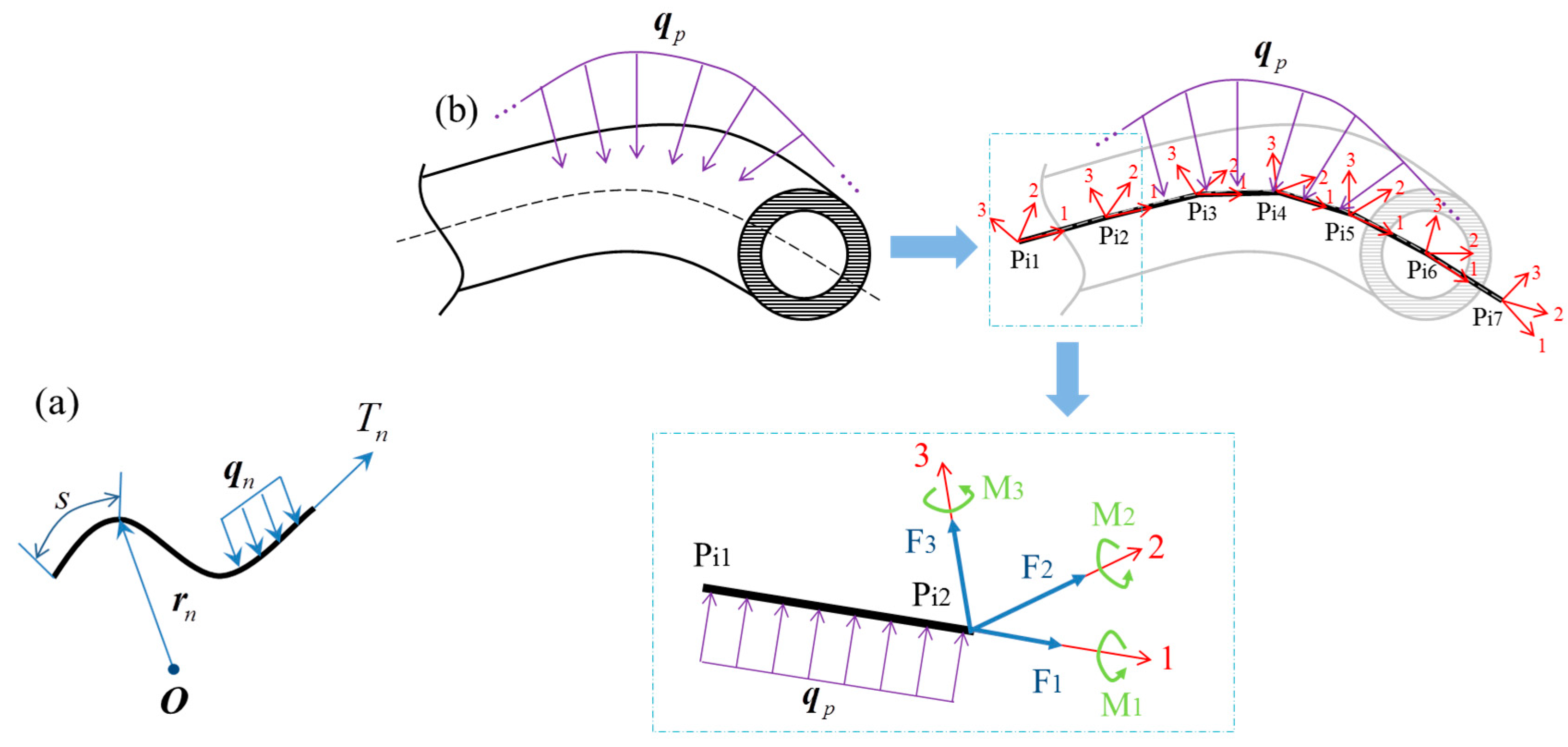
2.1. Basic Equations
2.2. Environmental Load
2.3. Environmental Model
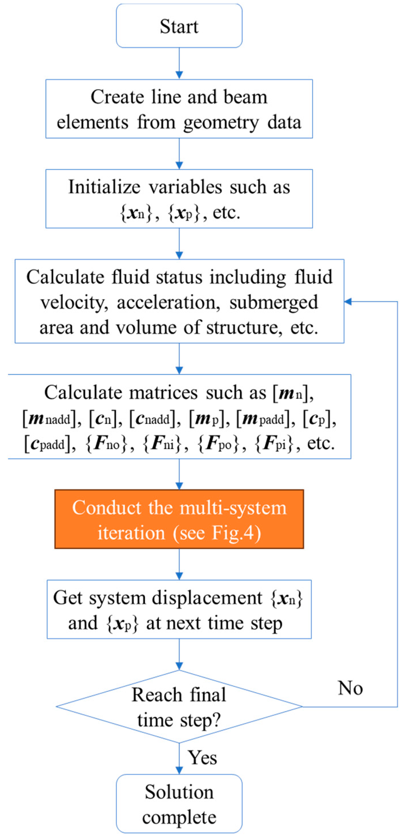
2.4. Coupling of Multiple Systems
3. Sea Trial
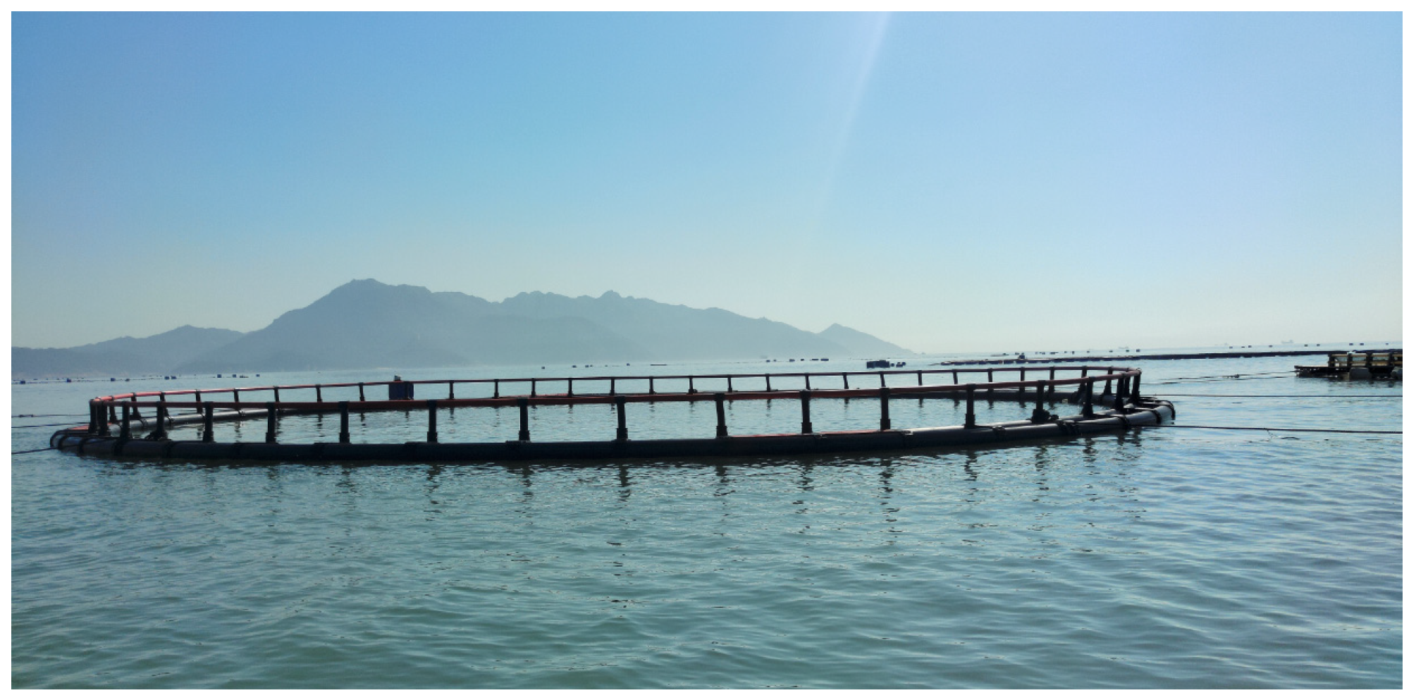
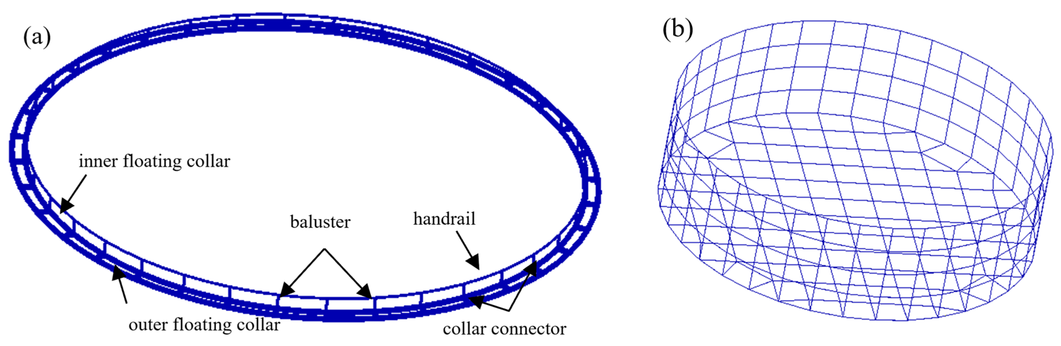
3.1. Tested Cage
3.2. Instruments
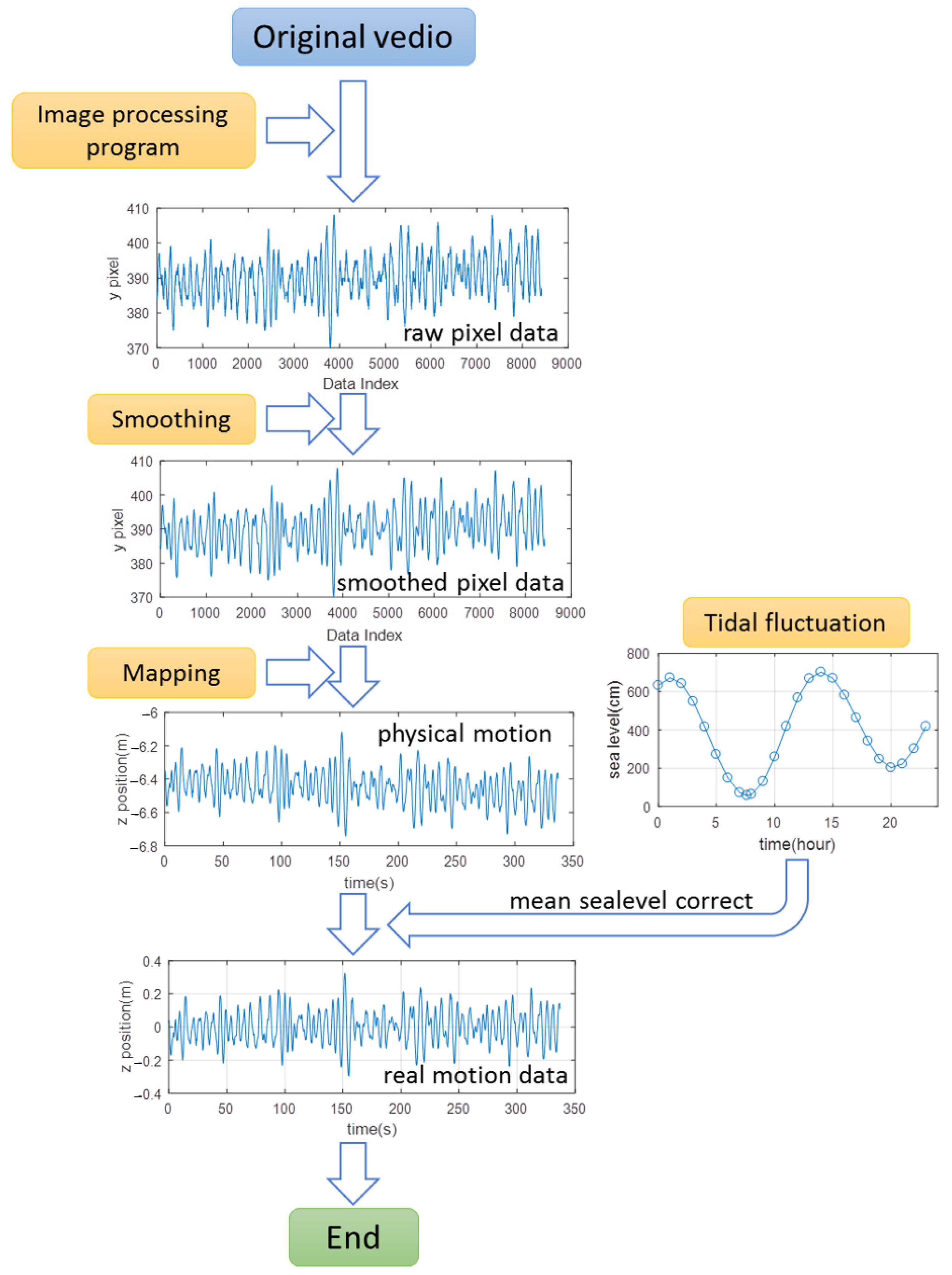
3.3. Measurement Method
4. Numerical Simulation
4.1. Simulation Model
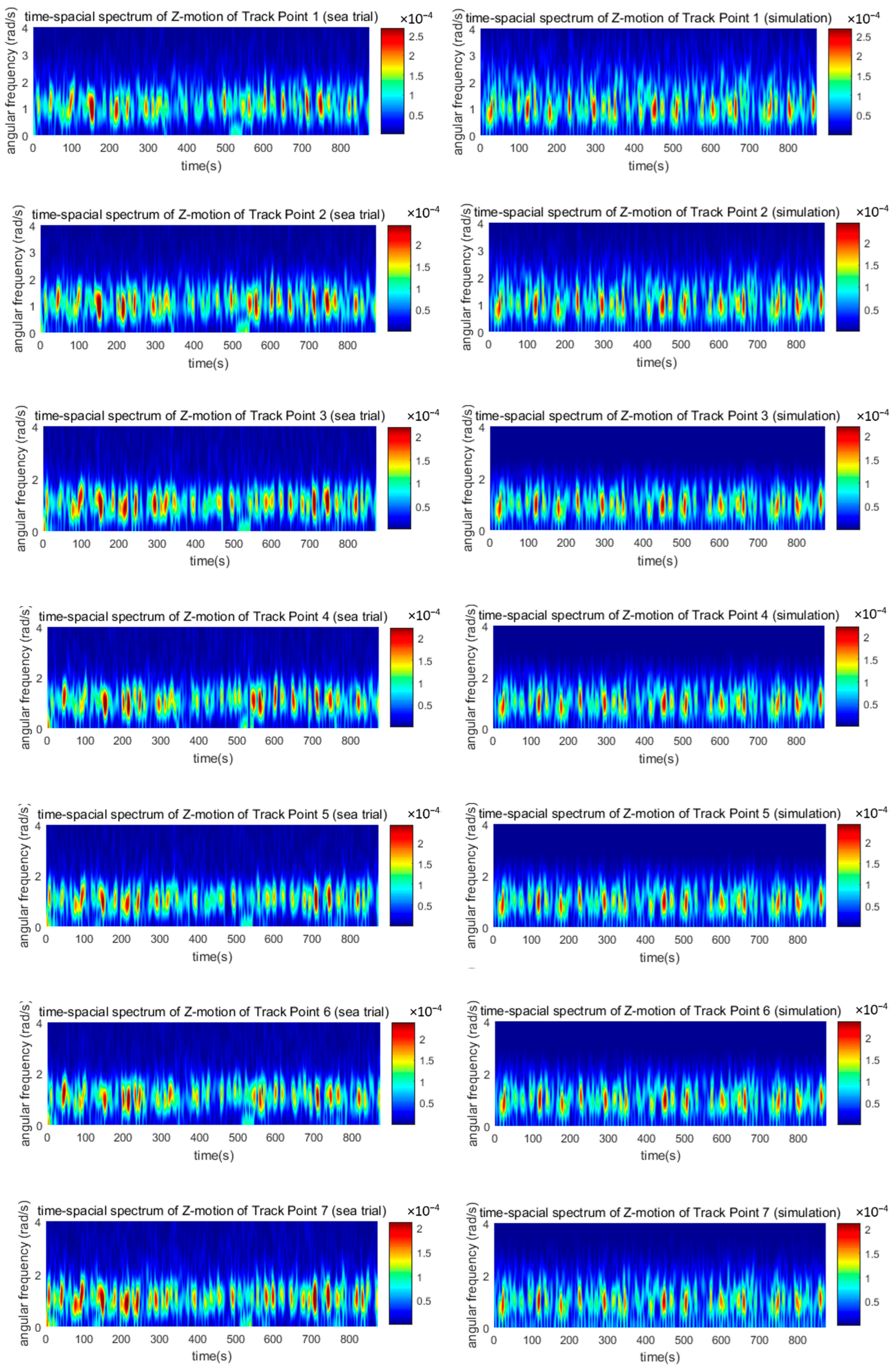
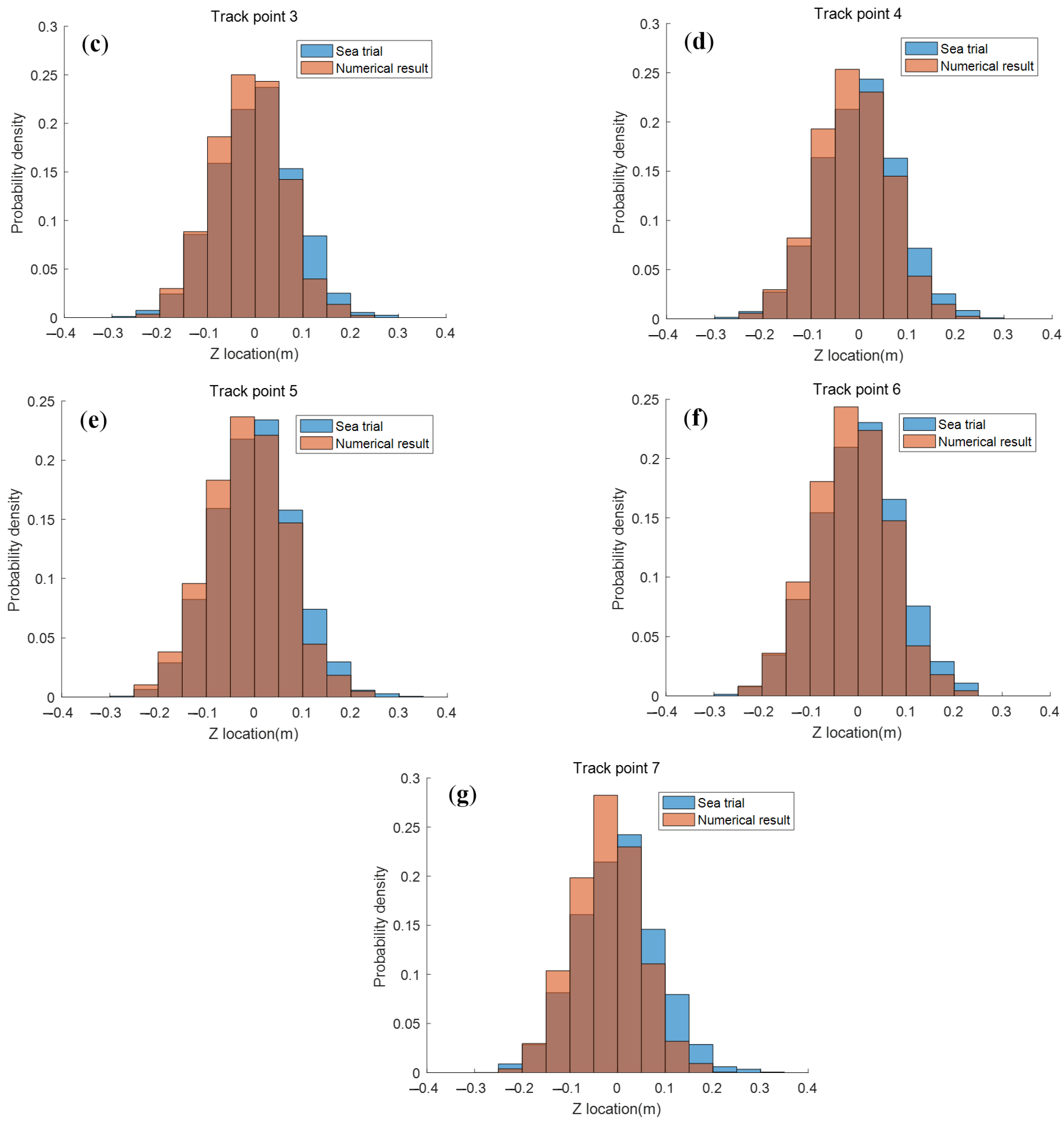
4.2. Validation
4.3. Simulation Cases
5. Results and Discussion
5.1. Motion
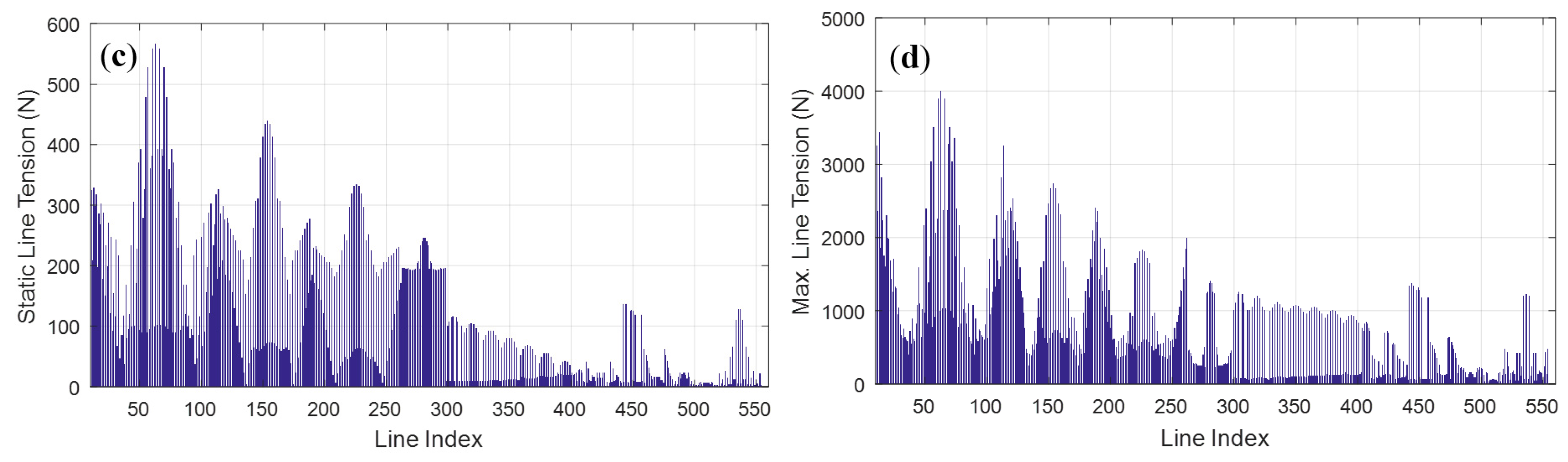
5.2. Tension of Mooring Lines and Net Lines
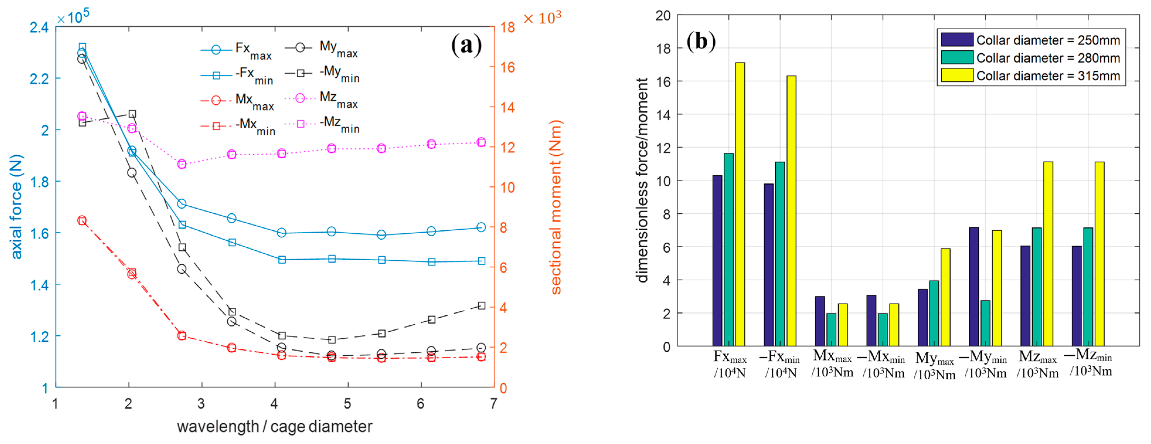
5.3. Structural Sectional Force
6. Conclusions
- The motion curves, time–frequency energy spectrums, and PDFs of the track points obtained by numerical simulation are in good agreement with those by the sea trial. The validity of the numerical method proposed in this article is therefore proved.
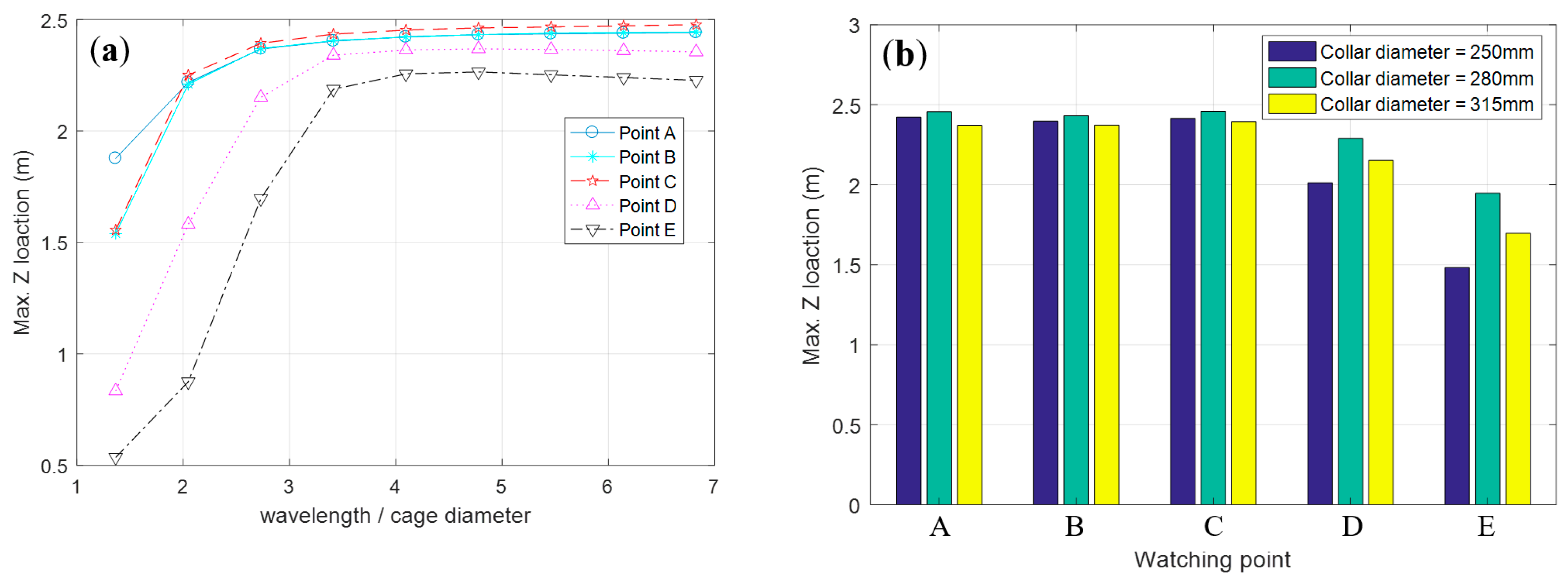
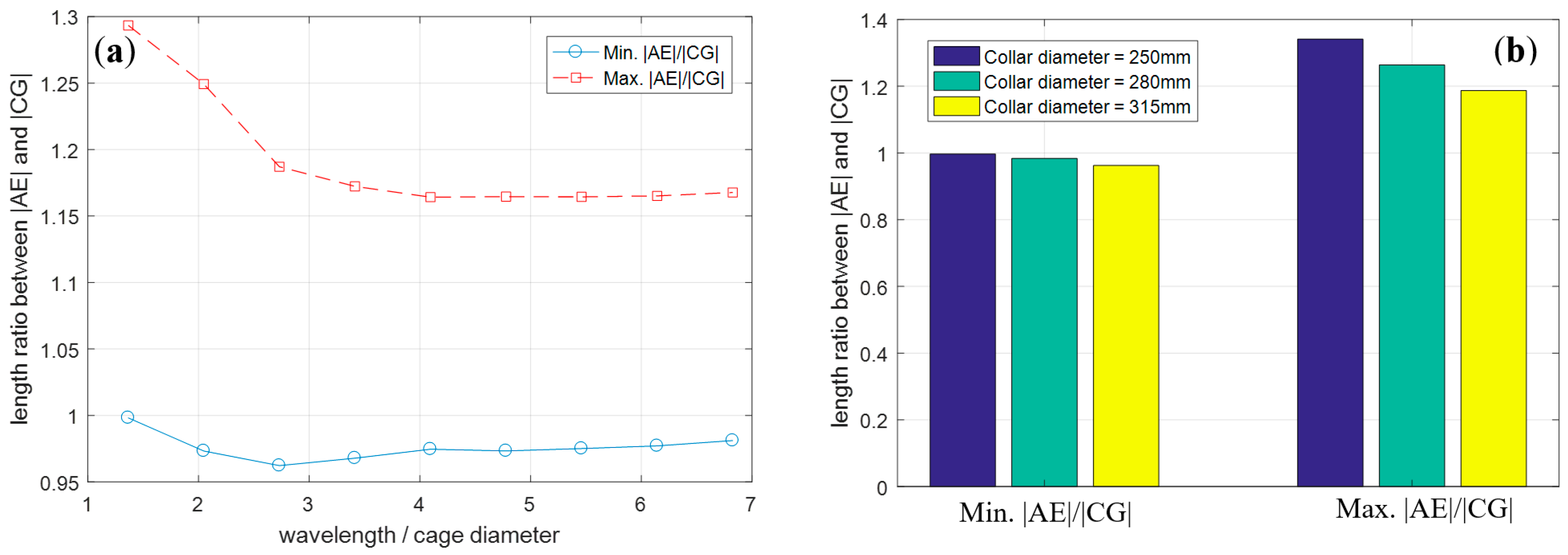
- Water entry may occur on the upstream side of the cage in extreme seas. When the wavelength is less than 4 times the cage diameter, a smaller wavelength can cause severe water entry. Excessive or insufficient stiffness of the cage can also exacerbate the water entry.
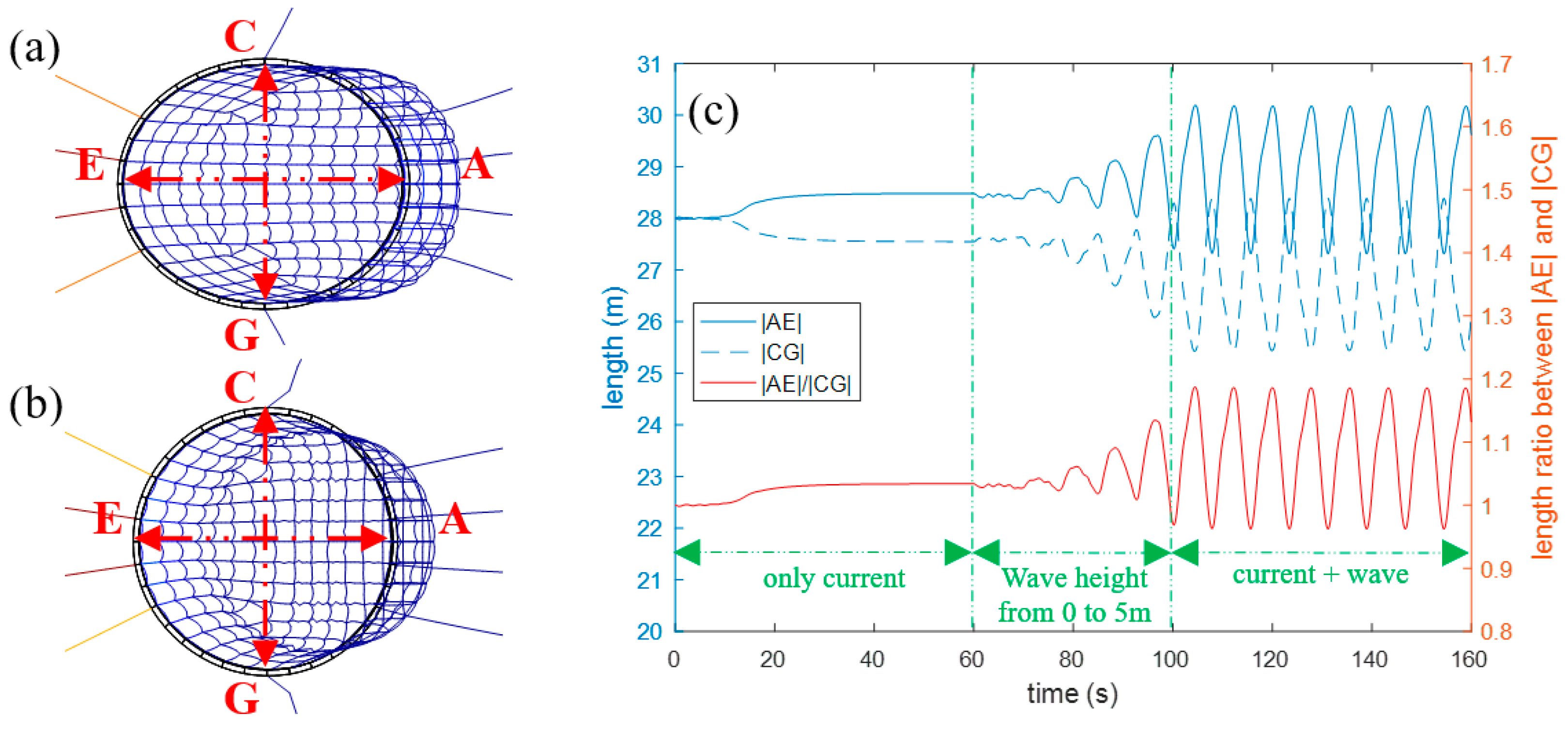
- The cage undergoes global deformation in extreme seas, which stretches along the current/wave direction and leads to an apparent reduction of the net volume. When the wavelength is less than 4 times the cage diameter, a smaller wavelength can cause severe deformation of the cage and a reduction of the net volume. As the stiffness of the cage decreases, the overall deformation of the cage becomes more pronounced, yet the reduction of the net volume declines.
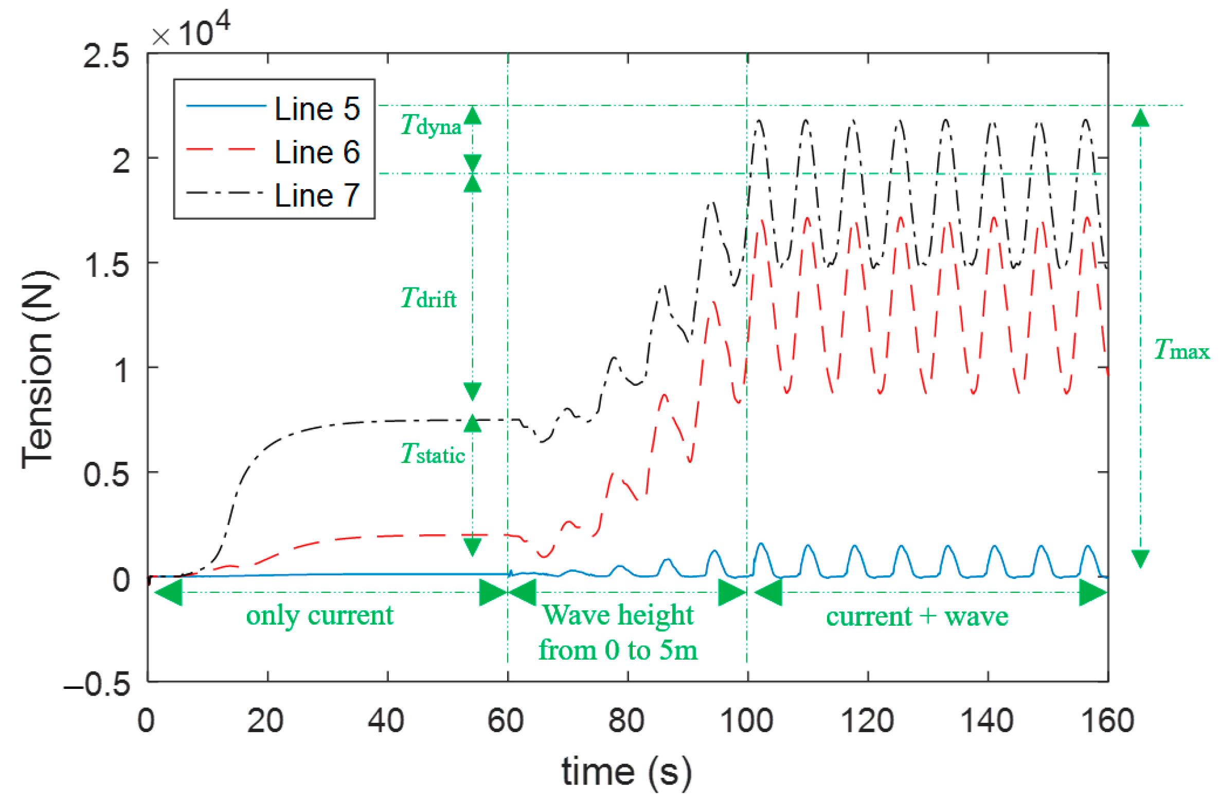
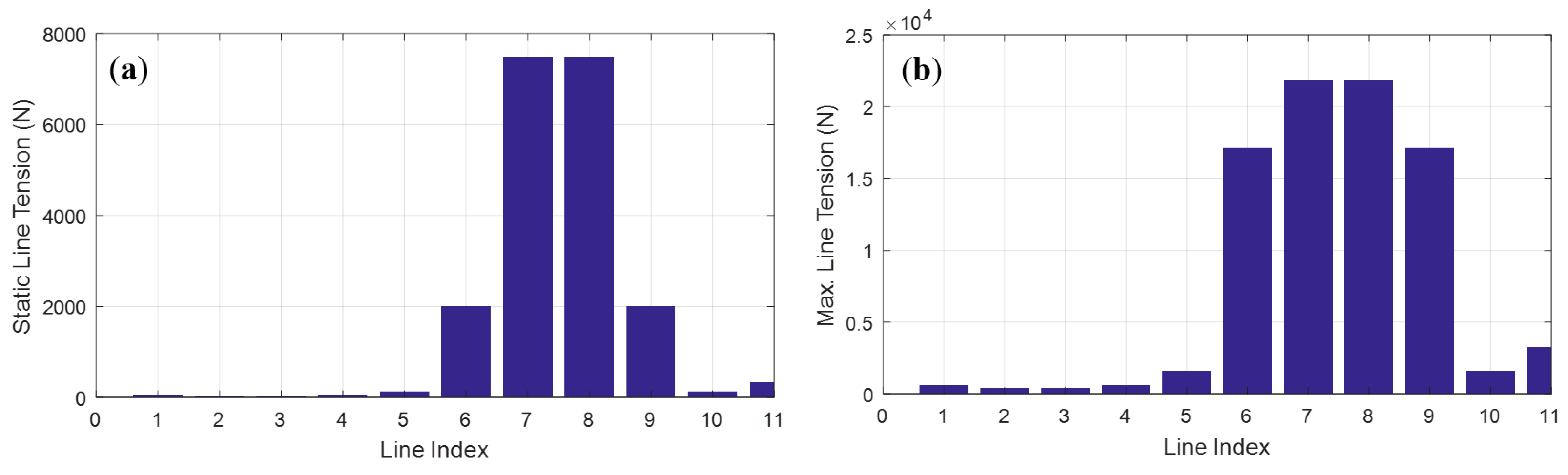
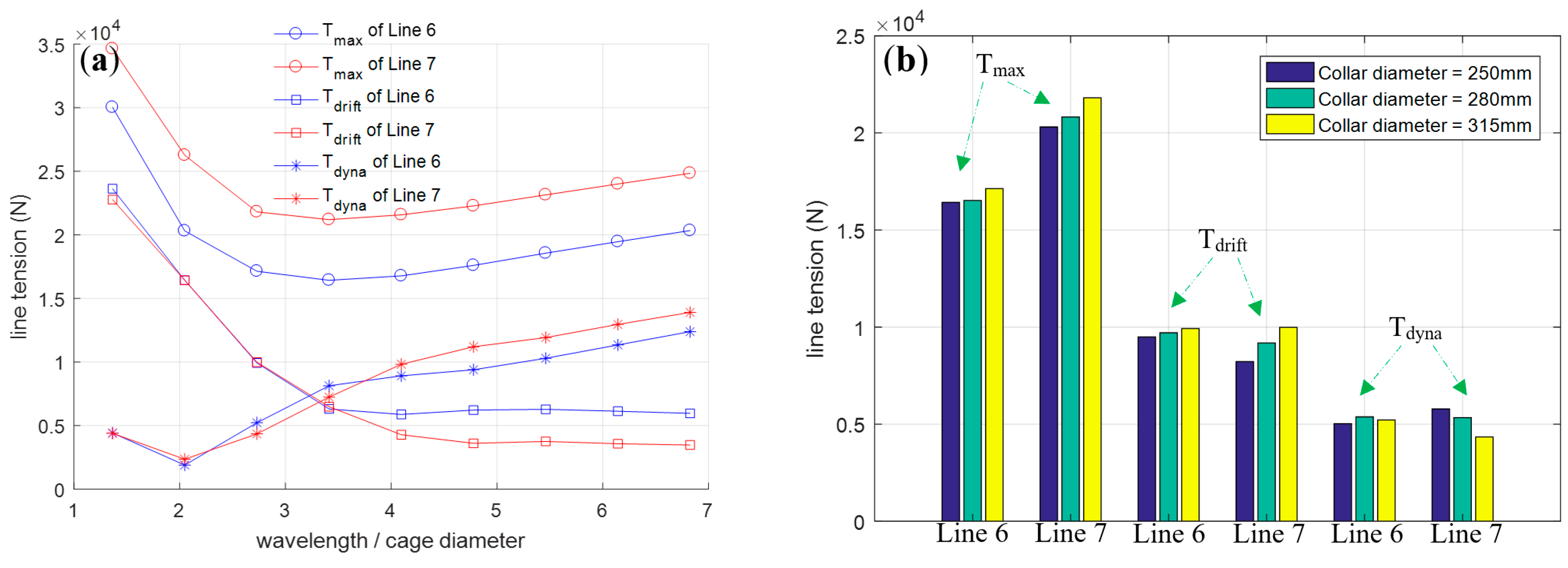
- As wavelength increases, Tdrift gradually decreases, Tdyna gradually increases, and Tmax decreases first and then increases, reaching its minimum when the wavelength equals 3.4 times the cage diameter. The wave-induced line tension Tdrift + Tdyna barely changes with wavelength, and the difference in tension between different lines mainly comes from the difference in their static tension Tstatic. As the stiffness of the cage increases, the tension of the mooring lines also increases, but the magnitude of the change is not significant.
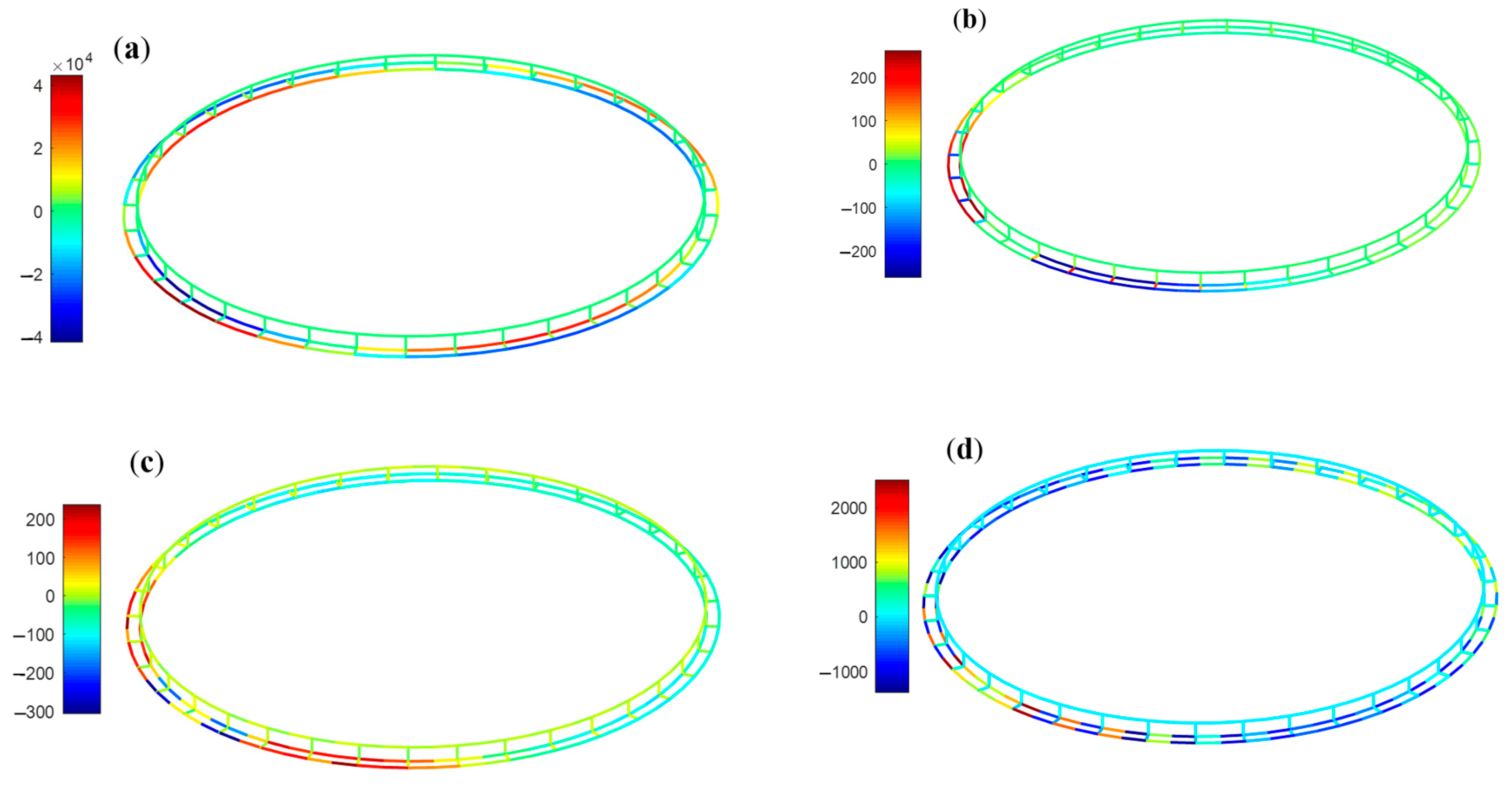
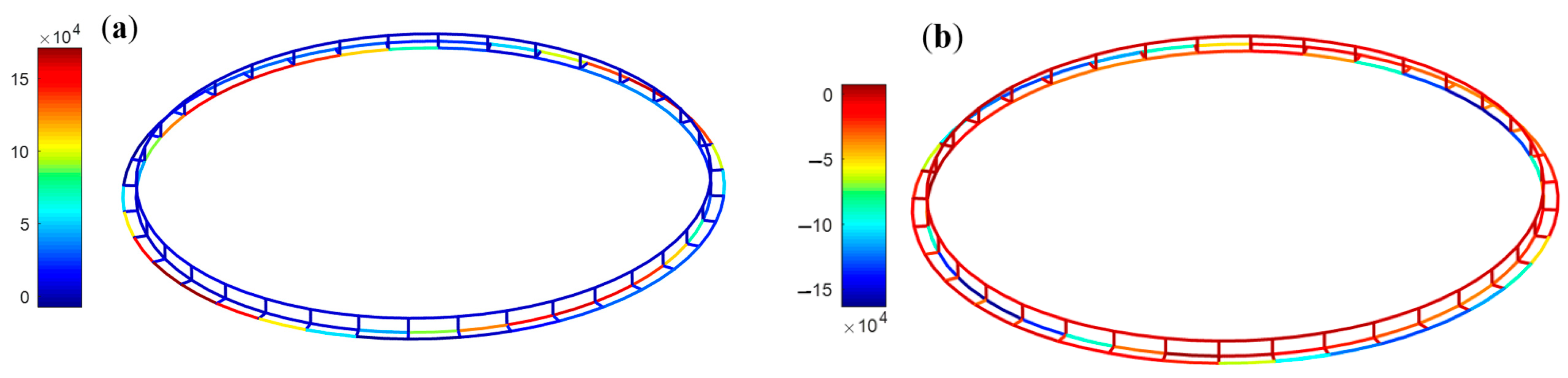
- Collars are the primary load-bearing structures of the cage, and the axial force is the dominant sectional load of the collars. Extreme axial forces occur at the east, west, south, and north positions of the cage, with alternating tension and compression at adjacent positions. The inner and outer collars form an entire composite beam by the collar connectors, and the signs of the axial forces of the inner and outer collars are always opposite. When the wavelength is less than 4 times the cage diameter, a smaller wavelength can cause greater sectional loads. Increasing the stiffness of the cage can significantly increase the sectional force of the cage.
- When the wavelength is greater than 4 times the cage diameter, the water-entry phenomenon, overall deformation, and sectional force of the cage are barely affected by the wavelength.
Author Contributions
Funding
Institutional Review Board Statement
Informed Consent Statement
Data Availability Statement
Conflicts of Interest
References
- Food and Agriculture Organization of the United Nations. The State of World Fisheries and Aquaculture. In Towards Blue Transformation; Food and Agriculture Organization of the United Nations: Rome, Italy, 2022. [Google Scholar]
- Guo, Y.C.; Mohapatra, S.C.; Soares, C.G. Review of developments in porous membranes and net-type structures for breakwaters and fish cages. Ocean Eng. 2020, 200, 107027. [Google Scholar] [CrossRef]
- Hu, J.; Zhao, Y.; Liu, P.L.F. A model for obliquely incident wave interacting with a multi-layered object. Appl. Ocean Res. 2019, 87, 211–222. [Google Scholar] [CrossRef]
- Ma, M.; Zhang, H.; Jeng, D.S.; Wang, C.M. A Semi-Analytical Model for Studying Hydroelastic Behaviour of a Cylindrical Cage under Wave Action. J. Mar. Sci. Eng. 2021, 9, 1445. [Google Scholar] [CrossRef]
- Mohapatra, S.C.; Bernardo, T.A.; Soares, C.G. Dynamic wave induced loads on a moored flexible cylindrical cage with analytical and numerical model simulations. Appl. Ocean Res. 2021, 110, 102591. [Google Scholar] [CrossRef]
- Chen, Y.Y.; Yang, B.D.; Chen, Y.T. Applying a 3-D image measurement technique exploring the deformation of cage under wave–current interaction. Ocean Eng. 2019, 173, 823–834. [Google Scholar] [CrossRef]
- Dong, S.; You, X.; Hu, F. Effects of wave forces on knotless polyethylene and chain-link wire netting panels for marine aquaculture cages. Ocean Eng. 2020, 207, 107368. [Google Scholar] [CrossRef]
- Wan, R.; Guan, Q.; Li, Z.; Hu, F.; Dong, S.; You, X. Study on hydrodynamic performance of a set-net in current based on numerical simulation and physical model test. Ocean Eng. 2020, 195, 106660. [Google Scholar] [CrossRef]
- Suzuki, K.; Takagi, T.; Shimizu, T.; Hiraishi, T.; Yamamoto, K.; Nashimoto, K. Validity and visualization of a numerical model used to determine dynamic configurations of fishing nets. Fish. Sci. 2003, 69, 695–705. [Google Scholar] [CrossRef]
- Bui, C.M.; Ho, T.X.; Khieu, L.H. Numerical study of a flow over and through offshore fish cages. Ocean Eng. 2020, 201, 107140. [Google Scholar]
- Cheng, H.; Ong, M.C.; Li, L.; Chen, H. Development of a coupling algorithm for fluid-structure interaction analysis of submerged aquaculture nets. Ocean Eng. 2022, 243, 110208. [Google Scholar]
- Su, B.; Kelasidi, E.; Frank, K.; Haugen, J.; Føre, M.; Pedersen, M.O. An integrated approach for monitoring structural deformation of aquaculture cages. Ocean Eng. 2021, 219, 108424. [Google Scholar] [CrossRef]
- Jónsdóttir, K.E.; Klebert, P.; Volent, Z.; Alfredsen, J.A. Characteristic current flow through a stocked conical sea-cage with permeable lice shielding skirt. Ocean Eng. 2021, 223, 108639. [Google Scholar] [CrossRef]
- Poizot, E.; Méar, Y.; Guillou, S.; Bibeau, E. High resolution characteristics of turbulence tied of a fish farm structure in a tidal environment. Appl. Ocean Res. 2021, 108, 102541. [Google Scholar] [CrossRef]
- Xu, Z.; Qin, H. Fluid-structure interactions of cage based aquaculture: From structures to organisms. Ocean Eng. 2020, 217, 107961. [Google Scholar] [CrossRef]
- Kristiansen, T.; Faltinsen, O.M. Experimental and numerical study of an aquaculture cage with floater in waves and current. J. Fluids Struct. 2015, 54, 1–26. [Google Scholar] [CrossRef]
- Huang, X.H.; Guo, G.X.; Tao, Q.Y.; Hu, Y.; Liu, H.Y.; Wang, S.M.; Hao, S.H. Dynamic deformation of the floating collar of a cage under the combined effect of waves and current. Aquac. Eng. 2018, 83, 47–56. [Google Scholar] [CrossRef]
- Zhao, Y.P.; Liu, H.F.; Bi, C.W.; Cui, Y.; Guan, C.T. Numerical study on the flow field inside and around a semi-submersible aquaculture platform. Appl. Ocean Res. 2021, 115, 102824. [Google Scholar] [CrossRef]
- Gansel, L.C.; Oppedal, F.; Birkevold, J.; Tuene, S.A. Drag forces and deformation of aquaculture cages—Full-scale towing tests in the field. Aquac. Eng. 2018, 81, 46–56. [Google Scholar] [CrossRef]
- Liu, S.; Bi, C.; Yang, H.; Huang, L.; Liang, Z.; Zhao, Y. Experimental study on the hydrodynamic characteristics of a submersible fish cage at various depths in waves. J. Ocean Univ. China 2019, 18, 701–709. [Google Scholar] [CrossRef]
- Dong, S.; Park, S.G.; Kitazawa, D.; Zhou, J.; Yoshida, T.; Li, Q. Model tests and full-scale sea trials for drag force and deformation of a marine aquaculture cage. Ocean Eng. 2021, 240, 109941. [Google Scholar] [CrossRef]
- Zhao, Y.P.; Bai, X.D.; Dong, G.H.; Bi, C.W. Deformation and stress distribution of floating collar of cage in steady current. Ships Offshore Struct. 2019, 14, 371–383. [Google Scholar] [CrossRef]
- Bi, C.-W.; Ma, C.; Zhao, Y.-P.; Xin, L.-X. Physical Model Experimental Study on the Motion Responses of a Multi-Module Aquaculture Platform. Ocean Eng. 2021, 239, 109862. [Google Scholar] [CrossRef]
- Bai, X.; Yang, C.; Luo, H. Hydrodynamic performance of the floating fish cage under extreme waves. Ocean Eng. 2021, 231, 109082. [Google Scholar] [CrossRef]
- Zhao, Y.P.; Bi, C.W.; Sun, X.X.; Dong, G.H. A prediction on structural stress and deformation of fish cage in waves using machine-learning method. Aquac. Eng. 2019, 85, 15–21. [Google Scholar] [CrossRef]
- Fan, Z.Q.; Liang, Y.H.; Zhao, Y.P. Review of the research on the hydrodynamics of fishing cage nets. Ocean Eng. 2023, 276, 114192. [Google Scholar] [CrossRef]
- Wilson, B.W. Elastic characteristics of moorings. J. Waterw. Harb. Div. 1967, 93, 27–56. [Google Scholar] [CrossRef]
- Klust, G. Fibre Ropes for Fishing Gear; Fishing News Books: London, UK, 1983. [Google Scholar]
- Zhan, J.M.; Hu, Y.Z.; Zhao, T.; Sun, M.G. Hydrodynamic experiment and analysis of fishing net. Ocean Eng. 2002, 20, 49–53+59. (In Chinese) [Google Scholar]
- Bessonneau, J.S.; Marichal, D. Study of the dynamics of submerged supple nets (applications to trawls). Ocean Eng. 1998, 25, 563–583. [Google Scholar] [CrossRef]
- Zhu, X.; Bi, Q.; Nicoll, R.; Li, X.; Zhu, Y.; Li, G. Cable tension formulas for gravity net cage arrays in current. Ocean Eng. 2024, 291, 116423. [Google Scholar] [CrossRef]
- DeCew, J.; Tsukrov, I.; Risso, A.; Swift, M.R.; Celikkol, B. Modeling of dynamic behavior of a single-point moored submersible fish cage under currents. Aquac. Eng. 2010, 43, 38–45. [Google Scholar] [CrossRef]
- Mousselli, A.H. Offshore Collarline Design, Analysis, and Methods; Pennwell Corp.: Tulsa, OK, USA, 1981. [Google Scholar]
- Shen, H.; Zhao, Y.P.; Bi, C.W.; Xu, Z. Nonlinear dynamics of an aquaculture cage array induced by wave-structure interactions. Ocean Eng. 2023, 269, 113711. [Google Scholar] [CrossRef]
- Su, W.; Zhan, J.M. Computational method for deformation of volume of net structure in current. Ocean Eng. 2007, 25, 93–100. (In Chinese) [Google Scholar]
- Daubechies, I. Ten Lectures on Wavelets; Society for Industrial and Applied Mathematics: Philadelphia, PA, USA, 1992. [Google Scholar]


| Parameter | Value | Parameter | Value |
|---|---|---|---|
| Perimeter of the outer collar (m) | 92 | Width of collar connector (mm) | 250 |
| Perimeter of the inner collar (m) | 88 | Shell thickness of collar connector (mm) | 20 |
| Diameter of the collar pipe (mm) | 315 | Diameter of the baluster pipe (mm) | 110 |
| Thickness of the collar pipe (mm) | 23.2 | Thickness of the baluster pipe (mm) | 10 |
| Space between two collars (mm) | 650 | Diameter of the handrail pipe (mm) | 95 |
| Size of each web (mm) | 35 × 35 | Thickness of the handrail pipe (mm) | 8.2 |
| Diameter of the web line (mm) | 2 | Height of the handrail (mm) | 800 |
| Depth of the entire net (m) | 8 | Diameter of the mooring line (mm) | 35 |
| Material of the net | PE | Length of each mooring line (m) | 64 |
| Number of sinkers on the net | 36 | Material of the mooring line | PE |
| In-water weight of each sinker on the net (kg) | 20 | Length of the projection of a mooring line on the water plane (m) | 55 |
| Picture | Parameter | Value |
|---|---|---|
 | Acoustic frequency | ≥400 KHz |
| Acoustic beams | one vertical, three slanted at 25° | |
| Beam opening angle | 1.7° | |
| Maximum depth | 100 m | |
| Wave height range | −15 to +15 m | |
| Wave accuracy (Hs) | <1% of measured value/1cm | |
| Wave accuracy (Dir) | 2° | |
| Wave period range | 0.5 to 30 s | |
| Current velocity range | ±10 m/s horizontal, ±5 m/s along beam | |
| Current accuracy | 1% of measured value ±0.5 cm/s |
| Picture | Parameter | Value |
|---|---|---|
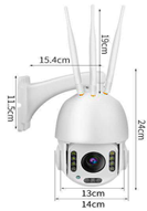 | Pixel | 2 to 5 million |
| Camera components | 1/3″ CMOS | |
| Rotation angle | horizontal 355°, vertical 105° | |
| Infrared distance | 60~120 m | |
| Optical zoom | 30× | |
| Focal length | 4~96 mm | |
| WIFI | Support, 802.11b/g/n | |
| Low illumination | 0.09 and [email protected] | |
| Electronic shutter | 1/50~1/10,000s |
| Re | <5 × 10³ | 5 × 10³ < Re < 1 × 10⁵ | 1 × 10⁵ < Re < 2.5 × 10⁵ | 2.5 × 10⁵ < Re < 5 × 10⁵ | >5 × 10⁵ |
|---|---|---|---|---|---|
| Cd | 1.3 | 1.2 | 1.53-Re/(3 × 105) | 0.7 | 0.7 |
| Track Point No. | 1 | 2 | 3 | 4 | 5 | 6 | 7 | |
|---|---|---|---|---|---|---|---|---|
| Sea trial (m) | Zmean | 0.23 | 0.22 | 0.19 | 0.19 | 0.20 | 0.20 | 0.19 |
| Z1/3 | 0.35 | 0.34 | 0.31 | 0.30 | 0.31 | 0.32 | 0.31 | |
| Z1/10 | 0.45 | 0.44 | 0.40 | 0.39 | 0.40 | 0.40 | 0.40 | |
| Numerical simulation (m) | Zmean | 0.24 | 0.21 | 0.19 | 0.19 | 0.21 | 0.20 | 0.18 |
| Z1/3 | 0.37 | 0.33 | 0.29 | 0.30 | 0.32 | 0.31 | 0.29 | |
| Z1/10 | 0.48 | 0.43 | 0.36 | 0.38 | 0.39 | 0.38 | 0.36 | |
| relative deviation | Zmean | 0.026 | −0.060 | 0.001 | 0.026 | 0.036 | 0.002 | −0.049 |
| Z1/3 | 0.071 | −0.029 | −0.072 | −0.030 | 0.014 | −0.041 | −0.073 | |
| Z1/10 | 0.076 | −0.026 | −0.095 | −0.046 | −0.031 | −0.056 | −0.097 | |
| Case No. | Current | Wave | Wavelength | Floating Collar Size |
|---|---|---|---|---|
| 1 | Velocity = 0.7 m/s Uniform current Direction = 0deg | Wave height = 5 m Wave direction = 0 deg Monochromatic regular wave Water depth = 16 m | 40 | D = 315 mm |
| 2 | 60 | |||
| 3 | 80 | |||
| 4 | 100 | |||
| 5 | 120 | |||
| 6 | 140 | |||
| 7 | 160 | |||
| 8 | 180 | |||
| 9 | 200 | |||
| 10 | 80 | D = 280 mm | ||
| 11 | D = 250 mm |
| Force | Type | Value | Belonging Structure | Position θ |
|---|---|---|---|---|
| Axial force Fx (kN) | Max. dynamic Fxmax | 171 | Outer floating collar | 180 deg |
| Min. dynamic Fxmin | −163 | Inner floating collar | 180 deg | |
| Max. Static Fxmax_static | 43.2 | Outer floating collar | 180 deg | |
| Min. Static Fxmin_static | −41.7 | Inner floating collar | 180 deg | |
| Torsional moment Mx (kNm) | Max. dynamic Mxmax | 2.56 | Inner floating collar | 145 deg |
| Min. dynamic Mxmin | −2.56 | Inner floating collar | −145 deg | |
| Max. Static Mxmax_static | 0.261 | Inner floating collar | 145 deg | |
| Min. Static Mxmin_static | −0.261 | Inner floating collar | −145 deg | |
| Vertical bending moment My (kNm) | Max. dynamic Mymax | 5.88 | Inner floating collar | 180 deg |
| Min. dynamic Mymin | −6.98 | Inner floating collar | 0 deg | |
| Max. Static Mymax_static | 0.237 | Outer floating collar | −145 deg | |
| Min. Static Mymin_static | −0.309 | Outer floating collar | 170 deg | |
| Horizontal bending moment Mz (kNm) | Max. dynamic Mzmax | 11.1 | Collar connector | −40 deg |
| Min. dynamic Mzmin | −11.1 | Collar connector | 40 deg | |
| Max. Static Mzmax_static | 2.51 | Inner floating collar | 170 deg | |
| Min. Static Mzmin_static | −1.38 | Outer floating collar | 145 deg | |
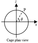 | Note: to describe the location where extreme sectional force occurs, the position of any point P is described by angle θ. | 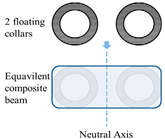 | Note: the inner and outer floating collars form a composite beam structure by the collar connectors. | |
Disclaimer/Publisher’s Note: The statements, opinions and data contained in all publications are solely those of the individual author(s) and contributor(s) and not of MDPI and/or the editor(s). MDPI and/or the editor(s) disclaim responsibility for any injury to people or property resulting from any ideas, methods, instructions or products referred to in the content. |
© 2024 by the authors. Licensee MDPI, Basel, Switzerland. This article is an open access article distributed under the terms and conditions of the Creative Commons Attribution (CC BY) license (https://creativecommons.org/licenses/by/4.0/).
Share and Cite
Zhang, X.; Fu, F.; Guo, J.; Qin, H.; Sun, Q.; Hu, Z. Numerical Simulation and On-Site Measurement of Dynamic Response of Flexible Marine Aquaculture Cages. J. Mar. Sci. Eng. 2024, 12, 1625. https://doi.org/10.3390/jmse12091625
Zhang X, Fu F, Guo J, Qin H, Sun Q, Hu Z. Numerical Simulation and On-Site Measurement of Dynamic Response of Flexible Marine Aquaculture Cages. Journal of Marine Science and Engineering. 2024; 12(9):1625. https://doi.org/10.3390/jmse12091625
Chicago/Turabian StyleZhang, Xiaoying, Fei Fu, Jun Guo, Hao Qin, Qian Sun, and Zhe Hu. 2024. "Numerical Simulation and On-Site Measurement of Dynamic Response of Flexible Marine Aquaculture Cages" Journal of Marine Science and Engineering 12, no. 9: 1625. https://doi.org/10.3390/jmse12091625