Identification of Floating Green Tide in High-Turbidity Water from Sentinel-2 MSI Images Employing NDVI and CIE Hue Angle Thresholds

Abstract

Remote sensing technology is widely used to obtain information on floating green tides, and thresholding methods based on indices such as the normalized difference vegetation index (NDVI) and the floating algae index (FAI) play an important role in such studies. However, as the methods are influenced by many factors, the threshold values vary greatly; in particular, the error of data extraction clearly increases in situations of high-turbidity water (HTW) (NDVI > 0). In this study, high spatial resolution, multispectral images from the Sentinel-2 MSI mission were used as the data source. It was found that the International Commission on Illumination (CIE) hue angle calculated using remotely sensed equivalent multispectral reflectance data and the RGB method is extremely effective in distinguishing floating green tides from areas of HTW. Statistical analysis of Sentinel-2 MSI images showed that the threshold value of the hue angle that can effectively eliminate the effect of HTW is 218.94°. A test demonstration of the method for identifying the floating green tide in HTW in a Sentinel-2 MSI image was carried out using the identified threshold values of NDVI > 0 and CIE hue angle < 218.94°. The demonstration showed that the method effectively eliminates misidentification caused by HTW pixels (NDVI > 0), resulting in better consistency of the identification of the floating green tide and its distribution in the true color image. The method enables rapid and accurate extraction of information on floating green tide in HTW, and offers a new solution for the monitoring and tracking of green tides in coastal areas.

1. Introduction

Green tide is a type of ecological disaster that occurs due to the fulminant reproduction and aggregation of macroalgae (e.g., Enteromorpha prolifera) in seawater under specific environmental conditions. The macroalgae float on the sea surface, and having strongly negative impacts on maritime transportation, coastal ecological environments, coastal aquaculture, tourism, etc., result in severe economic losses [1,2]. In all the 17 consecutive years since 2007, a large-scale green tide of Enteromorpha prolifera has occurred in the western Yellow Sea from May to August. Lasting for a long time and influencing wide sea areas, it is currently the largest scale green tide disaster in the world. Notably, the green tide in 2008 received widespread international attention owing to its influence on the sailing competition in the Olympic Games [3]. In recent years, the Chinese government has taken many measures to prevent and control the green tide, and the annual disaster has been controlled to some extent. However, since 2021, the green tide in the Yellow Sea has rebounded, so its prevention and control is a long-term, arduous task. Continuous and effective observation of floating green tides is therefore important, both for its scientific value and in practical terms of being able to prewarn of the occurrence of such tides.

Data obtained from remote-sensing technology is widely used to study floating green tides. The commonly used satellite data sources include MODIS, GOCI, HJ CCD, Landsat-8 OLI, GF WFV, and Sentinel-2 MSI [4,5,6,7,8]. The identification methods are mainly of two types. One type is vegetation index methods, which are based on the similarity of the reflectance spectra of green tide macroalgae and land vegetation; these include the normalized difference vegetation index (NDVI) [3,9,10,11,12,13], difference vegetation index (DVI) [5,14,15,16,17], and enhanced vegetation index (EVI) [18,19,20]. The other type is algae index methods, which have been specially established to identify floating green tides; these include the floating algae index (FAI) [4,6,19,21,22,23], the virtual-baseline floating macroalgae height (VB-FAH) [24,25], the alternative floating algae index (AFAI) [26], and the surface algal bloom index (SABI) [27]. Of these index methods, the NDVI and FAI are used widely owing to their ease of use and good identification of green tides. In particular, the NDVI metric is suitable for use with the data obtained by most satellite-based sensors, and thus it is the most commonly used [28]. When using the NDVI, the accuracy of identification of floating green tide depends primarily on the threshold value of the index selected. The threshold value is related to the difference in radiance in the satellite image between the green tide macroalgae and the surrounding seawater, and this varies greatly with environment [29]. In theory, the NDVI of water is less than zero, and that of green tide macroalgae is greater than zero. However, owing to many factors, such as the existing conditions when the satellite imagery is collected and the means used for data processing of the images, it may also be the case that the NDVI of nearshore high-turbidity water (HTW) is greater than zero. For such waters, if the NDVI threshold value is set to zero when extracting information on the floating green tide area, then the extraction result will be higher than the actual result. Therefore, when extracting information on floating green tide, researchers usually select a threshold value based on a priori knowledge. Furthermore, different researchers typically set different threshold values for the same image, so the extracted data will vary between researchers. For this reason, researchers have established various models to overcome this problem, such as the adaptive threshold model [29,30], machine learning model [31], and deep learning model [32,33,34]. However, these models are highly specialized and are difficult for general researchers to master, so they are not used widely.

In 1931, the International Commission on Illumination (CIE) developed a standard color space (CIE XYZ) and specified a two-dimensional xy chromaticity diagram. Individual colors can be described using chromaticity coordinates, with each color within the visible light range corresponding to a specific pair of chromaticity coordinates (x, y) [35]. Later, researchers defined a hue angle and established its relationship with the Forel-Ule index (FUI) [36,37]. Among other applications, to date, chromaticity coordinates, hue angle, and FUI have been applied successfully to the evaluation of the nutritional status of water [38,39] and the inversion of water color constituents [40,41,42], and the identification of coastal phytoplankton algal blooms and lake algal blooms [43,44,45,46]. The green tide, where the macroalgae float on the water surface, inevitably leads to an abnormal change of water color, and therefore, there is great potential to use the hue angle, etc., to used remotely sensed data to identify floating green tides.

In this study, first we analyzed the patterns of change in the NDVI and CIE hue angle of seawater and floating green tide based on the in situ measured differences between the spectra for seawater and floating green tide, and then formulated a means of identifying floating green tide using the thresholds of the NDVI and hue angle and examined the feasibility of the method. Then, we extracted the NDVI values of Sentinel-2 MSI L2A images not containing floating green tide and screened out the pixels representing HTW misidentified as representing floating green tide (NDVI > 0). By carrying out a statistical analysis of the distribution characteristic of hue angles of the misidentified pixels, we obtained a threshold value of the hue angle. Finally, we establish a method for identifying floating green tide in HTW based on threshold values of the NDVI and CIE hue angle that enables rapid and accurate extraction of information on floating green tide in HTW.

2. Data Source and Data Preprocessing

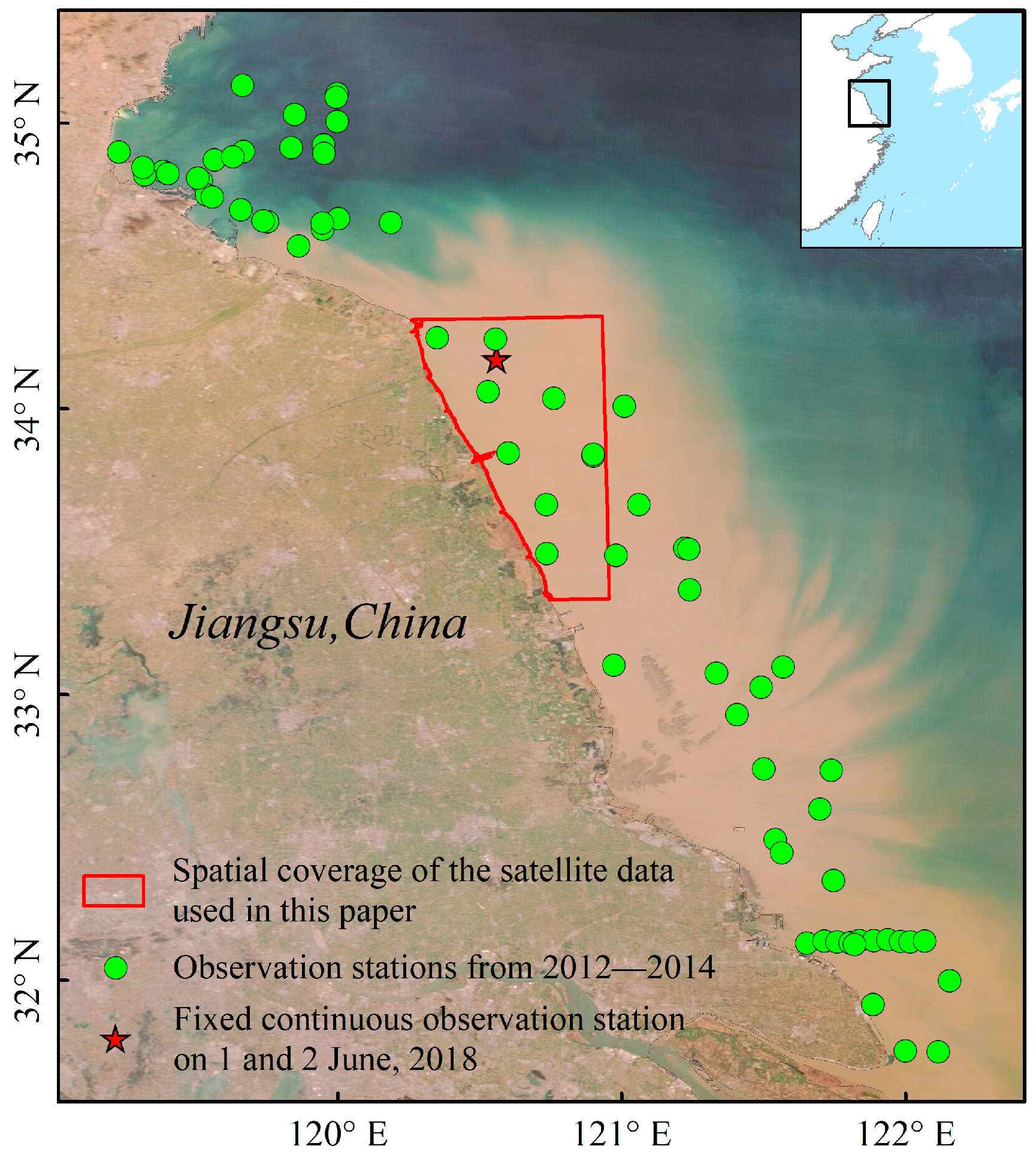
2.1. In Situ Measured Data

From 2012 to 2018, 174 in situ above-water reflectance spectra were acquired in the nearshore waters of Jiangsu Province, China, using an ASD spectrometer. The measurement was performed at a relative azimuth angle of 135° from the sun and at a nadir viewing angle of 40°. The reflectance was calculated as follows:

$$R\left(\lambda \right)={\displaystyle \frac{L_{\mathrm{t}}\left(\lambda \right)\cdot {\rho }_{\mathrm{r}}\left(\lambda \right)}{L_{\mathrm{p}}\left(\lambda \right)}}$$

(1)

where R(λ) is the reflectance of observation targets such as the seawater or floating green tide, L_t(λ) is the radiance of observation targets, L_p(λ) is the radiance of reflection standard board, ρ_r is the reflectance of reflection standard board.

The fixed station continuous observation of coastal sea areas at Yancheng, Jiangsu on 1 and 2 June 2018 yielded 105 reflectance spectra, including 77 of floating green tide and 28 of seawater. The other 69 reflectance spectra of seawater were acquired during a cross-section observation voyage made during 2012–2014. The distribution of the in situ optical observation stations and the spatial coverage of the satellite data are shown in Figure 1.

Based on the Sentinel-2 MSI spectral response function, the in situ hyperspectral reflectance was used to calculate the equivalent multispectral reflectance. The exact formula is as follows:

$$R\left({\lambda }_{\mathrm{i}}\right)={\displaystyle \frac{{{\displaystyle \int }}_{400}^{1000}R\left(\lambda \right)\cdot F_{\mathrm{s}}\left(\lambda \right)\cdot f\left({\lambda }_{\mathrm{i}}\right)\mathrm{d}\lambda }{{{\displaystyle \int }}_{400}^{1000}{F}_{\mathrm{s}}\left(\lambda \right)\cdot f\left({\lambda }_{\mathrm{i}}\right)\mathrm{d}\lambda }}$$

(2)

where R(λ_i) is the equivalent reflectance at the central wavelength λ_i, R(λ) is the in situ measured hyperspectral reflectance, F_s(λ) is the mean solar radiative flux at the top of the atmosphere, and f(λ_i) is the spectral response function at λ_i.

2.2. Satellite Data

The satellite data used in this study were Level-2A Sentinel-2 MSI surface reflectance data. The spatial resolution of Sentinel-2 MSI imagery is 10 m (for spatial resolution bands B2 (490 nm), B3 (560 nm), B4 (665 nm) and B8 (842 nm)), 20 m (B5 (705 nm), B6 (740 nm), B7 (783 nm), B8a (865 nm), B11 (1610 nm) and B12 (2190 nm)), and 60 m (B1 (443 nm), B9 (940 nm) and B10 (1375 nm)), and the revisit period is 5 days. The downloaded imagery was first resampled using the European Space Agency (ESA) SNAP (Sentinel Application Platform) to acquire reflectance data with 10 m spatial resolution. The reflectance in the seven bands B2 (490 nm), B3 (560 nm), B4 (665 nm), B5 (705 nm), B6 (740 nm), B7 (783 nm), and B8 (842 nm) was then used to calculate the NDVI and CIE hue angle. Information regarding the satellite data used in this study is shown in

Table 1. The satellite data used in this study.

Date	Data	Object
3 May 2022	S2A_MSIL2A_20220503T023551_N0400_R089_T51STT_20220503T061017	CIE hue angle threshold analysis
19 December 2022	S2A_MSIL2A_20221219T024121_N0509_R089_T51STT_20221219T060453
18 January 2023	S2A_MSIL2A_20230118T024031_N0509_R089_T51STT_20230118T055159
28 January 2023	S2A_MSIL2A_20230128T023951_N0509_R089_T51STT_20230128T055159
27 February 2023	S2A_MSIL2A_20230227T023641_N0509_R089_T51STT_20230227T055058
9 March 2023	S2A_MSIL2A_20230309T023531_N0509_R089_T51STT_20230309T055352
14 March 2023	S2B_MSIL2A_20230314T023529_N0509_R089_T51STT_20230314T045912
7 June 2022	S2B_MSIL2A_20220607T023549_N0400_R089_T51STT_20220607T052001	Method application
23 May 2023	S2B_MSIL2A_20230523T023539_N0509_R089_T51STT_20230523T045758
1 June 2024	S2A_MSIL2A_20240601T023551_N0510_R089_T51STT_20240601T074558

.

2.3. Calculation of the NDVI

The NDVI is commonly used as a means of extracting information about floating green tides from remotely sensed images. The formula for calculating the NDVI is

$$NDVI={\displaystyle \frac{R_{\mathrm{nir}\_\mathrm{red}\mathrm{edge}}-R_{\mathrm{red}}}{R_{\mathrm{nir}\_\mathrm{red}\mathrm{edge}}+R_{\mathrm{red}}}}$$

(3)

where R_{nir_red edge} is the reflectance of the near-infrared and red edge bands, and R_red is the reflectance of the red band. In this study, bands B4 and B6–B8 of the Sentinel-2 MSI imagery were selected for the calculation of the NDVI.

2.4. Calculation of the CIE Hue Angle

The CIE hue angle was calculated using the three standard tristimulus values X, Y, and Z of the CIE XYZ standard colorimetry system [35]. The formulae for calculating X, Y, and Z using the in situ hyperspectral reflectance (R(λ)) are

$$X=K{{\displaystyle \int }}_{380}^{700}S\left(\lambda \right)\cdot R\left(\lambda \right)\cdot \overline{x}\left(\lambda \right)d\lambda$$

(4)

$$Y=K{{\displaystyle \int }}_{380}^{700}S\left(\lambda \right)\cdot R\left(\lambda \right)\cdot \overline{y}\left(\lambda \right)d\lambda$$

(5)

$$Z=K{{\displaystyle \int }}_{380}^{700}S\left(\lambda \right)\cdot R\left(\lambda \right)\cdot \overline{z}\left(\lambda \right)d\lambda$$

(6)

$$K=100/{{\displaystyle \int }}_{380}^{700}S\left(\lambda \right)\cdot \overline{y}\left(\lambda \right)d\lambda$$

(7)

where S(λ) is the relative spectral energy distribution of the irradiation light source, usually taken as a wavelength-independent constant; $\stackrel{-}{x}\left(\lambda \right)$, $\stackrel{-}{y}\left(\lambda \right)$, and $\stackrel{-}{z}\left(\lambda \right)$ are the CIE color-matching functions, which are constants; and K is the adjustment factor.

The values of X, Y, and Z were calculated using the Sentinel-2 MSI L2A data for five visible light bands (B1–B5), using the linear intercept method [47]:

$$X=11.756R\left(443\right)+6.423R\left(490\right)+53.696R\left(560\right)+32.028R\left(665\right)+0.529R\left(705\right)$$

(8)

$$Y=1.744R\left(443\right)+22.289R\left(490\right)+65.702R\left(560\right)+16.808R\left(665\right)+0.192R\left(705\right)$$

(9)

$$Z=62.696R\left(443\right)+31.101R\left(490\right)+1.778R\left(560\right)+0.015R\left(665\right)+0.000R\left(705\right)$$

(10)

The Sentinel-2 MSI L2A data for RGB bands were transformed to the CIE tristimulus values X, Y, and Z as follows [37,38]:

$$X=1.1302R\left(490\right)+1.7517\left(560\right)+2.7689R\left(665\right)$$

(11)

$$Y=0.0601R\left(490\right)+4.5907R\left(560\right)+1.0000R\left(665\right)$$

(12)

$$Z=5.5934R\left(490\right)+0.0565R\left(560\right)+0.0000R\left(665\right)$$

(13)

The normalized chromaticity coordinates x and y were calculated from CIE tristimulus values X, Y, and Z as follows:

$$x=X/\left(X+Y+Z\right)$$

(14)

$$y=Y/\left(X+Y+Z\right)$$

(15)

Any color can be described by the two values x and y, and the CIE xy chromaticity diagram [38] shows all the colors in the visible range. Finally, the hue angle α can be found from the chromaticity coordinates (x, y) by using the bivariate arctangent function (arctan2) and the following equation:

$$\alpha ={\displaystyle \frac{\arctan 2(x-1/3,y-1/3)\cdot 180}{\mathsf{\pi }}}+180$$

(16)

3. Mechanistic Analysis of Identification Method

3.1. Difference in Characteristic Spectrum between Floating Green Tide and HTW

Measured reflectance spectra of floating green tides with different coverages (low, medium, and high, which refer to how much of the area of the green tide is covered by floating macroalgae), HTW, turbid water, and clean water are shown in Figure 2. The reflectance spectra for floating green tides exhibit reflectance valleys due to strong absorption by chlorophyll-a in the red band (B4), and very significant reflectance peaks in the red edge bands (B5–B7) and near-infrared band (B8). The heights of the peaks and valleys are related to the coverage of the floating green tide within the field of view of the spectrometer. The height of the reflectance peaks for the floating green tides increases constantly with the increase in coverage of the tide, and the reflectance valley declines gradually. In the visible region of the spectrum (400–700 nm), the HTW has the highest reflectance, followed by the turbid water and the floating green tides; the clean water has the lowest reflectance. In the red edge and near-infrared bands, the high-coverage floating green tide has the highest reflectance, followed by the mid-coverage floating green tide and HTW; the low-coverage floating green tide and clean water have the lowest reflectance. There is only a slight difference in the red edge and near-infrared bands in the spectra for the HTW and low-coverage floating green tide, but a clear difference is seen in the spectra in the visible region.

Owing to the significant spectral characteristics of the floating green tides in the red, red edge, and near-infrared bands, the NDVI values of the typical reflectance spectra shown in Figure 2 were calculated using the equivalent reflectance values acquired by the Sentinel-2 MSI in the red edge bands (B5–B7), near-infrared band (B8), and red band (B4). The results (

Table 2. NDVI values for typical water bodies and floating green tides of different coverages calculated based on red edge and near-infrared bands.

Target Type	Spatial Resolution Band
	B5	B6	B7	B8
Clean water	−0.3943	−1.4495	−1.3281	−1.3253
Turbid water	−0.1996	−0.8570	−0.8599	−0.9075
HTW	0.0093	−0.0649	−0.0407	−0.0678
Low-coverage floating green tide	0.1756	0.0267	0.0127	−0.0439
Mid-coverage floating green tide	0.3350	0.4471	0.4446	0.4143
	0.3434	0.4773	0.4760	0.4503
High-coverage floating green tide	0.6816	0.8065	0.8052	0.7960
	0.7474	0.8882	0.8896	0.8861
	0.7567	0.9196	0.9240	0.9226

) show that, similar to conclusions drawn in many previously reported studies, the NDVI values calculated based on all the red edge and infrared bands are less than zero for the clean water and turbid water and greater than zero for mid-coverage and high-coverage floating green tides. It is worth noting that, for HTW, some NDVI values calculated based on band B5 data are greater than zero, indicating that the strong scattering effect of the HTW increases the reflectance in this band. Therefore, NDVI values calculated based on band B5 data will cause partial HTW to be misidentified as floating green tide. For low-coverage floating green tide, some NDVI values calculated based on band B8 data are less than zero, indicating that in this case, the typical spectral characteristic is not significant in the red and near-infrared bands. Therefore, the NDVI values calculated based on band B8 data will not enable identification of partial low-coverage floating green tide. However, if band B6 or B7 data are added for the calculation, all the NDVI values obtained will be greater than zero, indicating that it is necessary to add the data for these red edge bands, B6 and B7, in order to identify floating green tide using the NDVI method. After comprehensive consideration, we calculated the NDVI values by combining the maximum reflectance values in bands B6–B8 with the value in band B4, which is used to identify floating green tide in HTW. In this way, the results obtained will be more accurate and reliable.

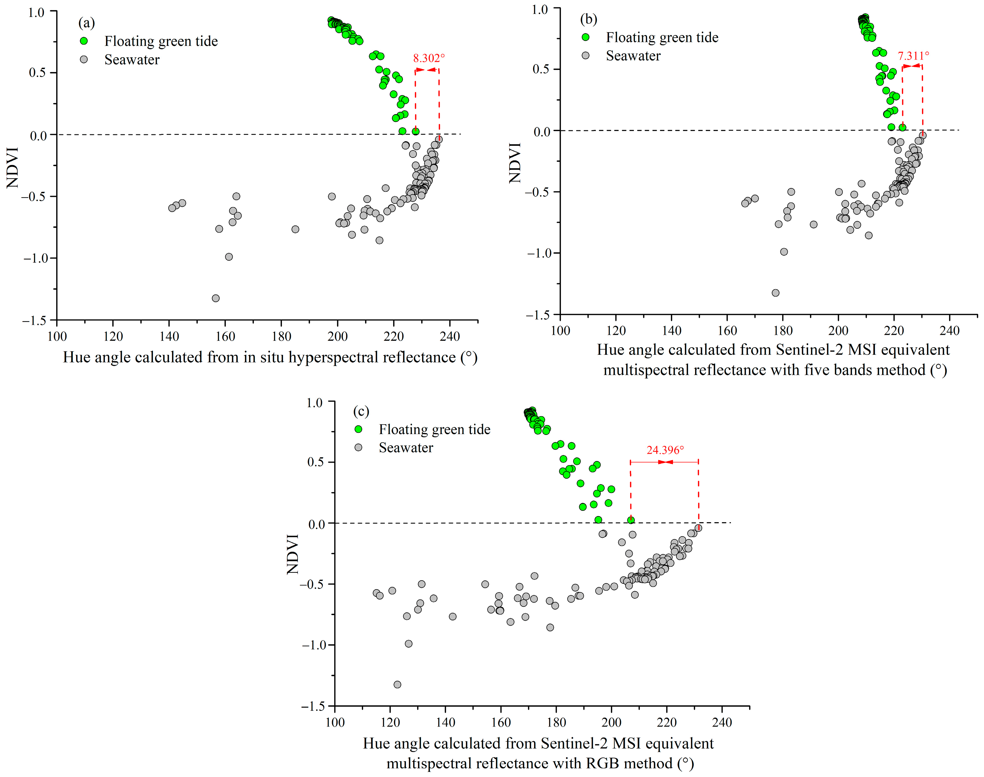
3.2. Different in Hue Angle between Floating Green Tide and Turbid Water

Floating green tide and turbid water are very visually different in terms of color, and it is therefore potentially possible to distinguish between them using their threshold of hue angles. The hue angles of floating green tide and seawater were calculated separately using the in situ measured hyperspectral reflectance and the corresponding multispectral reflectance in the five visible bands (B1–B5) or the three RGB bands (B2–B4) of the Sentinel-2 MSI; then, the hue angle versus NDVI scatterplots were drawn (Figure 3). It was found that the sample points for floating green tide and those for seawater are distributed on opposite sides of the x axis (NDVI = 0). The sample points for HTW and low-coverage floating green tide are closer to the x axis than other sample points because their NDVI values are close to zero; however, the hue angle of floating green tide is significantly less than that of HTW. Further statistics showed that the hue angles for HTW and low-coverage floating green tide calculated using the in situ measured hyperspectral reflectance (Figure 3a) have a minimum difference of 8.302°, and those calculated using the equivalent multispectral reflectance in the five visible bands of Sentinel-2 MSI (Figure 3b) have a minimum difference of 7.311°. If the equivalent multispectral reflectance in the three RGB bands is used to calculate hue angle (Figure 3), the minimum difference in hue angle between floating green tide and HTW is increased, reaching 24.396°. Therefore, a better distinction between HTW and floating green tide can be drawn by using the hue angle calculated using the three RGB bands of Sentinel-2 MSI.

4. Determination of the NDVI and CIE Hue Angle Thresholds

The above analysis of in situ measured data shows that the addition of data for the red edge bands (B6 and B7) to the calculation of the NDVI improves the correct identification of floating green tide, and the introduction of the hue angle improves the distinction between HTW and floating green tide, thus reducing the misidentification rate. In practical applications, there are usually some factors of uncertainty in the preprocessing of satellite image, such as atmospheric correction, resulting in some deviation in the reflectance data obtained from such satellite images, and so the problem of the NDVI value of HTW being greater than zero is exacerbated [48]. Therefore, it is crucial to effectively distinguish between HTW and floating green tide. Here we postulate that introducing the hue angle to eliminate the influence of HTW on the NDVI threshold can solve the problem that HTW is misidentified as floating green tide if its NDVI is greater than zero, further improving the accuracy of identification of floating green tide in HTW. Next, we discuss in detail the setting of the thresholds for the NDVI and hue angle based on the Sentinel-2 MSI L2A image data.

4.1. NDVI Threshold

The Sentinel-2 MSI L2A image acquired on 23 May 2023 is used as an example (Figure 4). It can be seen from the figure that when the NDVI is set to >0, most of the pixels of the floating green tide area can be identified accurately; however, a large number of pixels of the HTW area are misidentified as pixels of floating green tide, and some pixels of floating green tide with very low coverage are not identified because their NDVI < 0. In general, the problem of misidentification of HTW with NDVI > 0 is solved by constantly increasing the NDVI threshold. However, while removing the pixels of HTW without floating green tide, such a method will also cause the pixels of floating green tide with 0 < NDVI < a given threshold (greater than zero) to be removed erroneously, resulting in a decreased identified area of floating green tide, thus greatly reducing the identification accuracy. Similarly, if those pixels of very low-coverage floating green tide need to be retained, it is required to constantly reduce the NDVI threshold. This will cause more HTW to be misidentified as floating green tide, resulting in a greatly increased identified area, thus evidently lowering the identification accuracy.

As the pixels of very low-coverage floating green tide themselves cover only a very small area of the green tide, it is believed that these pixels have a very small influence on the error in the identified floating green tide area and can be neglected. Therefore, in this study, the NDVI threshold was set to zero; in other words, it was deemed that all the NDVI values of floating green tide are greater than zero, so the pixels of very low-coverage floating green tide with NDVI values less than zero were neglected, and the misidentified pixels of HTW with NDVI > 0 were removed by the hue angle threshold.

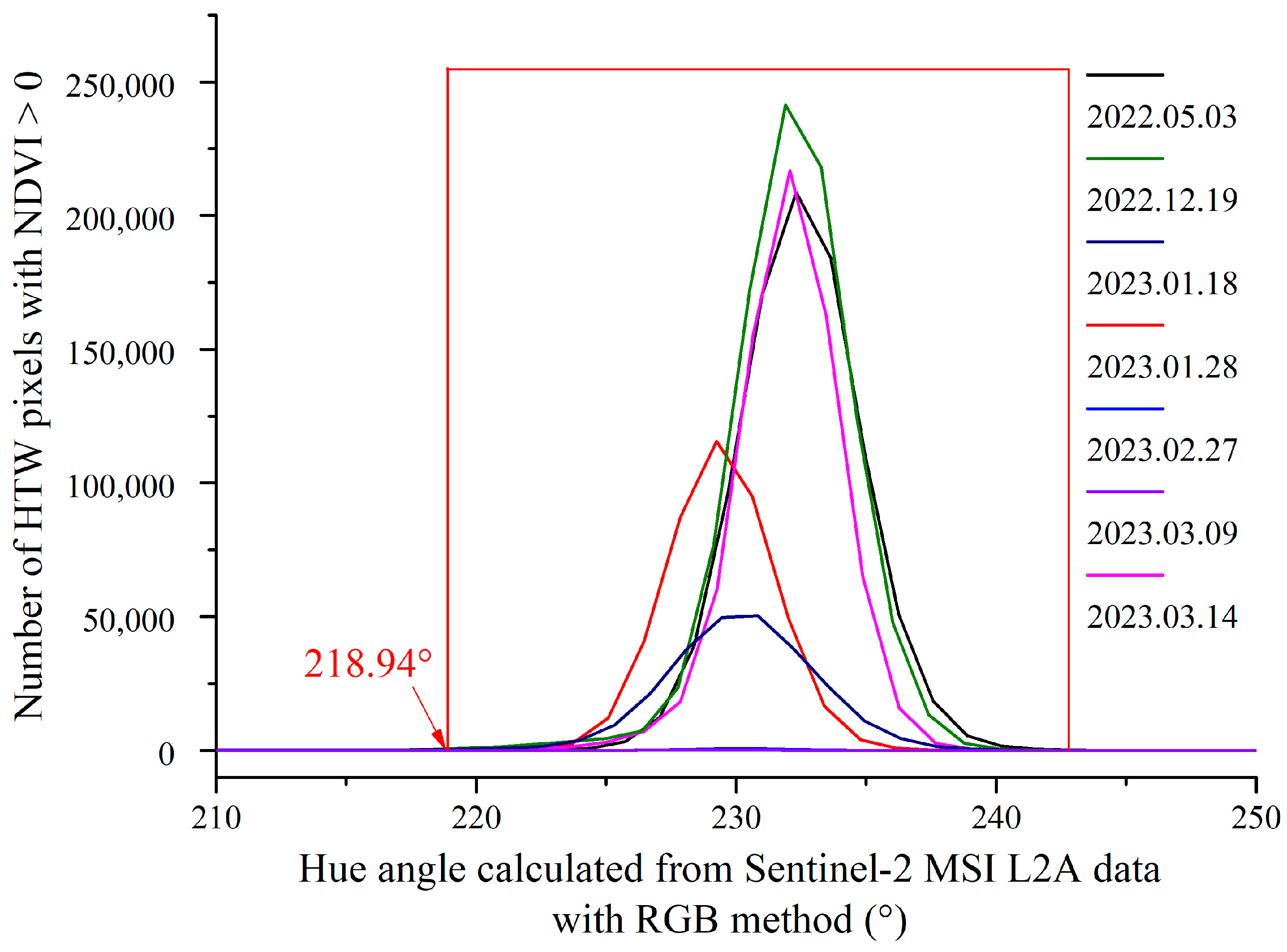
4.2. CIE Hue Angle Threshold

To more effectively remove the HTW pixels misidentified as pixels of floating green tide in Sentinel-2 MSI image, a suitable CIE hue angle threshold needs to be selected. In this study, seven satellite images without floating green tide obtained in the study area during 2022–2023 were chosen, the hue angles were calculated, and the distribution of pixel counts at different hue angles was plotted (Figure 5). The distribution diagram shows that the number of pixels with NDVI > 0 varies greatly between the images, ranging from hundreds to over 900,000, and the pixels are mainly related to the actual distribution area of HTW in the image. The number of HTW pixels with NDVI > 0 exhibits a normal distribution relationship with the hue angle, and their hue angles are concentrated in the range 218.94–242.79°. Therefore, a hue angle of 218.94° is the critical value for removal of HTW pixels. Consequently, we determined that when the hue angle is ≥218.94°, the pixel represents HTW. When the hue angle is <218.94° and the NDVI is >0, the pixel represents floating green tide.

HTW pixels were removed from seven images based on a hue angle threshold of 218.94°. The statistical results of this process (

Table 3. Statistics on the effectiveness of the hue angle threshold for the removal of HTW pixels with NDVI > 0.

Image Date	Total Number of Pixels	Number of Pixels Removed	Removal Rate	Number of Pixels Not Removed	Non-Removal Rate
3 May 2022	905,110	904,699	99.95%	411	0.05%
19 December 2022	940,850	940,214	99.93%	636	0.07%
18 January 2023	259,933	254,483	97.90%	5450	2.10%
28 January 2023	425,700	425,081	99.85%	619	0.15%
27 February 2023	2524	2275	90.13%	249	9.87%
9 March 2023	802	633	78.93%	169	21.07%
14 March 2023	709,838	709,377	99.94%	461	0.06%

) show that for satellite images having relatively many pixels with NDVI > 0 (wide HTW distribution), the removal rate of HTW pixels is generally over 99.8%, except for the image obtained on 18 January 2023 for which the removal process was slightly poor (removal rate 97.90%). For some satellite images having very few pixels with NDVI > 0 (very little HTW distribution), the removal rate was relatively low; however, very few pixels were not removed (<250 pixels in each image), so their influence can be neglected. On the whole, setting the hue angle threshold at 218.94° effectively eliminates the influence of HTW.

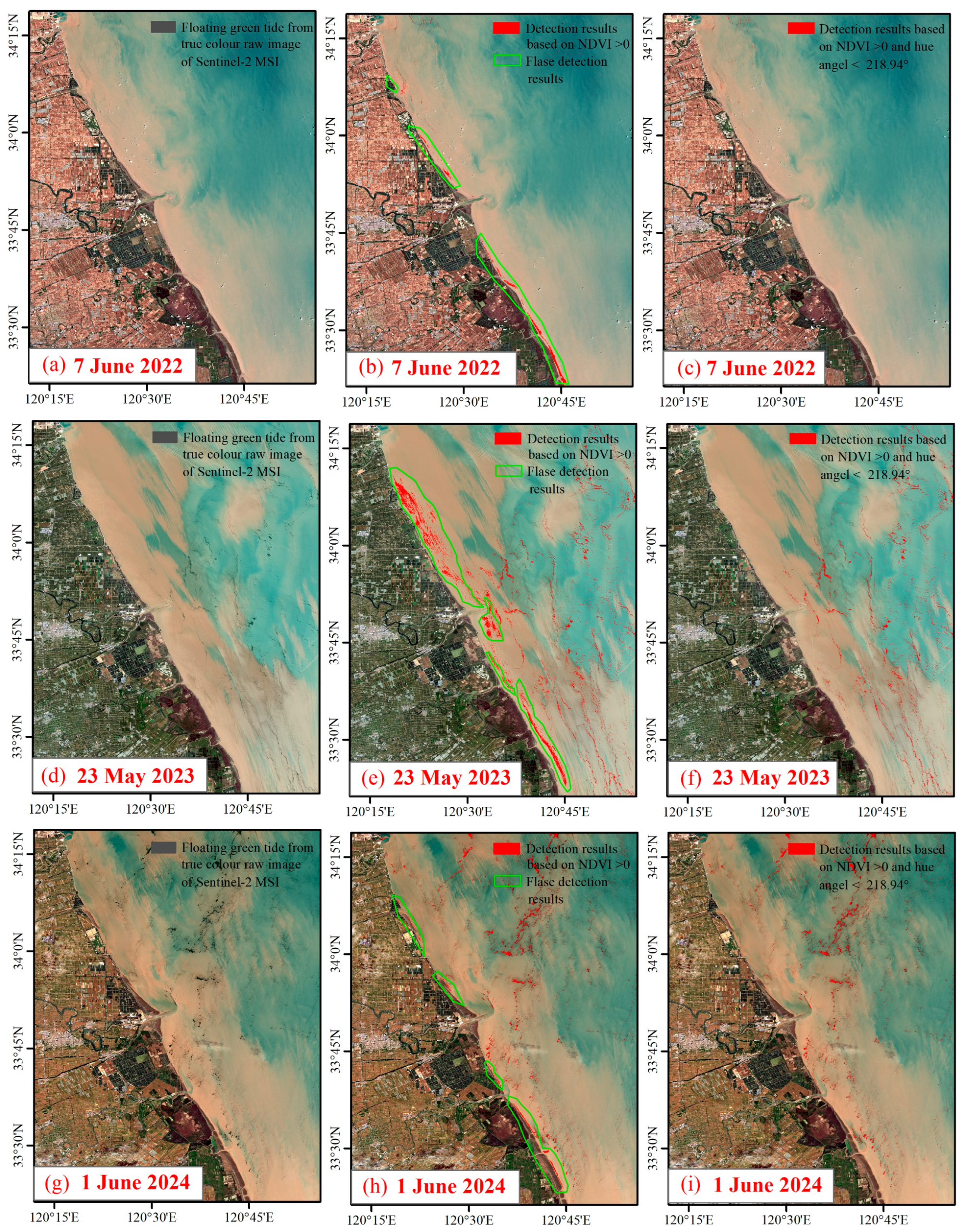
5. Demonstration of Method

Using the Sentinel-2 MSI L2A image obtained on 7 June 2022, 23 May 2023, and 1 June 2024 as examples, floating green tides were extracted from the images using the traditional NDVI thresholding method (NDVI > 0) and the combined NDVI and hue angle thresholding method proposed in this study (NDVI > 0 and hue angle < 218.94°). The identification results are shown in Figure 6. It can be seen that, in the true color raw image (Figure 6a), the floating green tide displays as dark green and is distributed in the coastal seawater in a banded or scattered manner. The results extracted using the traditional NDVI thresholding method (Figure 6b) show that there are a large number of misidentified pixels in the nearshore HTW area. However, the identification results extracted using the method proposed in this study (Figure 6c) exhibit very good consistency with the distribution status of floating green tide in the raw image, indicating that using the hue angle threshold in addition to the NDVI threshold can effectively remove the HTW pixels misidentified as floating green tide. The combined NDVI and hue angle thresholding method gives good extraction results for images of different years, especially when there is a small amount of cloud present in the 1 June 2023 image, and still performs well, which fully demonstrates the very nice adaptability of the method.

To further compare the performance of the traditional NDVI thresholding method and that of the method proposed in this study, we looked at the following factors:

• The identification error rate—the ratio of the number of HTW pixels misidentified as floating green tide to the number of floating green tide pixels;
• The loss rate—the ratio of the number of floating green tide pixels removed owing to a constantly increased NDVI threshold to the number of floating green tide pixels;
• The total misidentification rate—to the sum of the identification error rate and the loss rate.

The visual identification on an image of areas covered by floating green tides having different coverages is extremely challenging, and it cannot be ensured that all floating green tide pixels are identified 100% accurately. However, the results obtained using the method proposed in this study (NDVI > 0 and CIE hue angle < 218.94°) agree very closely with the distribution of floating green tide seen in the true color raw image, so the results obtained using our method were taken as the true values of the number of floating green tide pixels, and were used to calculate the method-evaluation factors. As an example of extraction results on 23 May 2023, it can be seen from the results in

Table 4. Error statistics for floating green tide identification results under different NDVI threshold conditions.

No.	NDVI Threshold	Identification Error Rate	Loss Rate	Total Misidentification Rate
1	0	101.76%	0.00%	101.76%
2	0.01	62.74%	2.41%	65.14%
3	0.02	35.08%	4.84%	39.91%
4	0.03	19.56%	7.15%	26.71%
5	0.04	11.84%	9.36%	21.20%
6	0.05	7.97%	11.46%	19.42%
7	0.06	5.99%	13.50%	19.49%
8	0.07	4.84%	15.48%	20.32%
9	0.08	3.96%	17.44%	21.40%
10	0.09	3.23%	19.32%	22.55%
11	0.10	2.64%	21.14%	23.78%
12	0.15	1.00%	29.58%	30.58%
13	0.20	0.39%	36.97%	37.35%
14	0.25	0.16%	43.42%	43.57%
15	0.30	0.06%	49.13%	49.19%

that as the NDVI threshold increases, the number of HTW pixels misidentified as floating green tide increases and the identification error rate decreases from 101.76% to 0.06%. However, as the NDVI threshold increases, an increasing number of pixels of low-coverage floating green tide are removed as well, with the loss rate increasing from 0 to 49.13%. The total misidentification rate first decreases from 101.76% to 19.42% and then increases to 49.19%. This fully indicates that the traditional NDVI thresholding method has many disadvantages. Even if the threshold value is adjusted constantly, the error will still persist, being 19.42% at a minimum.

The above analysis reveals that the single NDVI threshold method for extracting the floating green tide requires constant adjustment of the NDVI threshold in order to achieve a better extraction effect, which is a relatively cumbersome process, but the actual extraction accuracy is still difficult to ensure. The hue angle (or chromaticity coordinates) serves as the comprehensive indicator of water radiance information and represents one of the key quantitative parameters for assessing water color, which has been successfully applied to the extraction of harmful algal blooms. Nevertheless, the study of extracting floating green tide using hue angle has not yet been reported, and in this study, NDVI was combined with hue angle for the first time, and very good application results were achieved. The CIE hue angle shows significant potential in marine ecological disaster monitoring using remote sensing methods.

6. Discussion

6.1. Selection of Identification Factors

There are numerous methods for identifying floating green tides. In the present study, we selected just two identification factors, namely, the NDVI and the hue angle. As the NDVI is a fundamental factor and is highly suitable for identifying floating green tides, it is obvious that it should be selected as an identification factor. However, whether there is another factor that could be substituted for the hue angle or would be a better factor than the hue angle requires further discussion. The purpose of the hue angle threshold is to filter out the HTW pixels that influence the identification of floating green tide. In theory, any factor that is sensitive to the water turbidity (e.g., reflectance or reflectance combination) could be used.

The Sentinel-2 MSI L2A image obtained on 19 December 2022 (which shows no floating green tide) was selected and the values of the following turbidity-sensitive factors were extracted: the hue angle values corresponding to pixels with NDVI > 0, the reflectance values in bands B2–B8, and the B4/B3 reflectance ratio (normally used for the inversion of the concentration suspended matter or turbidity). The distribution of the pixel counts within the variation interval of the above factors was plotted (Figure 7). It can be seen from the figure that for the reflectance values in bands B2–B8 and the B4/B3 reflectance ratio (Figure 7b–i), in addition to a very significant main peak, there is weak oscillation or a secondary peak in the low-value zone. This has an unfavorable influence on the determination of the threshold of a turbidity-sensitive factor. If the oscillation or secondary peak is neglected, the set threshold will be high, resulting in incomplete removal of HTW pixels. If the influence of the oscillation or secondary peak is taken into account, the set threshold will be low, causing excessive removal of HTW pixels, thus resulting in loss of floating green tide pixels. Therefore, none of the above turbidity-sensitive factors would be a suitable identification factor. Conversely, the distribution of pixel counts of the hue angle (Figure 7a) has only one significant main peak and no oscillation or secondary peak, so the hue angle threshold setting is stable and accurate and the hue angle is the best identification factor.

6.2. Suitability of Other Satellite Data Sources

The identification method established in this study has high application value. However, the band settings, atmospheric correction level, and so on can vary between different types of high spatial resolution satellite images, and this will result in poor comparability of calculated NDVI or hue angle values obtained from different image types. Consequently, if the NDVI and hue angle thresholds determined in this study using Sentinel-2 MSI L2A images are to be used for other satellite data sources, a study should first be carried out to verify their suitability. If they are unsuitable, specific thresholds should be determined for the images being used, using a calculation process similar to the one described in this paper.

7. Conclusions

A novel remote sensing method based on the NDVI and CIE hue angle is proposed for the identification of floating green tide in HTW on Sentinel-2 MSI images.

The red edge bands (B6 (740 nm) and B7 (783 nm)) are more effective for identifying low-coverage floating green tide using the NDVI method. In this study the NDVI was calculated by identifying the maxima of the reflectance in bands B6–B8 and combining it with the reflectance in band B4 (665 nm). The CIE hue angle calculated using the equivalent multispectral reflectance in the three RGB bands can effectively distinguish between floating green tide and HTW, and can enlarge the difference in hue angle between floating green tide and HTW to the maximum extent.

Compared with the reflectance in individual bands or the reflectance ratio between two bands, the CIE hue angle has a better performance in eliminating the influence of HTW with NDVI > 0. If the hue angle threshold is set at 218.94°, when the number of HTW pixels in an image is very large, the pixel removal rate is basically over 99.8%, whereas when the number of HTW pixels is small (<3000), the number of HTW pixels not removed is less than 250 (i.e., the error can be neglected).

A method for identifying floating green tide in HTW on Sentinel-2 MSI images was proposed (i.e., NDVI > 0 and CIE hue angle < 218.94). The test demonstration of the method showed that the method can effectively remove HTW pixels with NDVI > 0, and the results obtained exhibit very good consistency with the distribution status of floating green tide seen in the true color raw image. The proposed method is simple, user-friendly, and can be easily mastered by general monitors. Most importantly, the method enables rapid and accurate extraction of information on floating green tide in HTW, and so has important practical application value to coastal management and ecological conservation efforts.

In future work, we plan to integrate the method presented in this paper with the floating green tide outbreak prediction model through programming, so as to achieve a systematic and automatic monitoring and assessment capability of floating green tide, and provide technical support for the supervision of marine ecological disasters.

References

1. Wang, X.H.; Li, L.; Bao, X.; Zhao, L.D. Economic cost of an algae bloom cleanup in China’s 2008 Olympic sailing venue. Eos Trans. Am. Geophys. Union. 2009, 90, 238–239. [Google Scholar] [CrossRef]
2. Hu, C.; Cannizzaro, J.; Carder, K.L.; Muller-Karger, F.E.; Hardy, R. Remote detection of Trichodesmium blooms in optically complex coastal waters: Examples with MODIS full-spectral data. Remote Sens. Environ. 2010, 114, 2048–2058. [Google Scholar] [CrossRef]
3. Hu, C.M.; He, M.X. Origin and offshore extent of floating algae in Olympic sailing area. Eos Trans. Am. Geophys. Union. 2008, 89, 302–303. [Google Scholar] [CrossRef]
4. Hu, L.B.; Hu, C.M.; He, M.X. Remote estimation of biomass of Ulva prolifera macroalgae in the Yellow Sea. Remote Sens. Environ. 2017, 192, 217–227. [Google Scholar] [CrossRef]
5. Cui, T.W.; Liang, X.J.; Gong, J.L.; Tong, C.; Xiao, Y.; Liu, R.; Zhang, X.; Zhang, J. Assessing and refining the satellite-derived massive green macro-algal coverage in the Yellow Sea with high resolution images. ISPRS J. Photogramm. Remote Sens. 2018, 144, 315–324. [Google Scholar] [CrossRef]
6. Sun, D.Y.; Chen, Y.; Wang, S.Q.; Zhang, H.; Qiu, Z.; Mao, Z.; He, Y. Using Landsat 8 OLI data to differentiate Sargassum and Ulva prolifera blooms in the South Yellow Sea. Int. J. Appl. Earth Obs. Geoinf. 2021, 98, 102302. [Google Scholar] [CrossRef]
7. Wang, X.H.; Xing, Q.G.; An, D.Y.; Meng, L.; Zheng, X.; Jiang, B.; Liu, H. Effects of spatial resolution on the satellite observation of floating macroalgae blooms. Water 2021, 13, 1761. [Google Scholar] [CrossRef]
8. Zheng, L.; Wu, M.Q.; Cui, Y.T.; Tian, L.; Yang, P.; Zhao, L.; Xue, M.; Liu, J. What causes the great green tide disaster in the South Yellow Sea of China in 2021. Ecol. Indic. 2022, 140, 108988. [Google Scholar] [CrossRef]
9. Keesing, J.K.; Liu, D.; Fearns, P.; Garcia, R. Inter-and intra-annual patterns of Ulva prolifera green tides in the Yellow Sea during 2007–2009, their origin and relationship to the expansion of coastal seaweed aquaculture in China. Mar. Pollut. Bull. 2011, 62, 1169–1182. [Google Scholar] [CrossRef]
10. Xing, Q.G.; Tosi, L.; Braga, F.; Gao, X.; Gao, M. Interpreting the progressive eutrophication behind the world’s largest macroalgal blooms with water quality and ocean color data. Nat. Hazards 2015, 78, 7–21. [Google Scholar] [CrossRef]
11. Sun, X.; Wu, M.Q.; Xing, Q.G.; Song, X.; Zhao, D.; Han, Q.; Zhang, G. Spatio-temporal patterns of Ulva prolifera blooms and the corresponding influence on chlorophyll-a concentration in the Southern Yellow Sea, China. Sci. Total Environ. 2018, 640, 807–820. [Google Scholar] [CrossRef] [PubMed]
12. Li, D.X.; Gao, Z.Q.; Wang, Z.C. Analysis of the reasons for the outbreak of Yellow Sea green tide in 2021 based on long-term multi-source data. Mar. Environ. Res. 2022, 178, 105649. [Google Scholar] [CrossRef] [PubMed]
13. Zhang, B.W.; Guo, J.Z.; Li, Z.W.; Cheng, Y.; Zhao, Y.; Boota, M.W.; Zhang, Y.; Feng, L. Identifying the spatio-temporal variations of Ulva prolifera disasters in all life cycle. J. Water Clim. Chang. 2021, 13, 629–644. [Google Scholar] [CrossRef]
14. Xu, F.X.; Gao, Z.Q.; Shang, W.T.; Jiang, X.; Zheng, X.; Ning, J.; Song, D. Validation of MODIS-based monitoring for a green tide in the Yellow Sea with the aid of unmanned aerial vehicle. J. Appl. Remote Sens. 2017, 11, 012007. [Google Scholar] [CrossRef]
15. Xing, Q.; Wu, L.; Tian, L.; Cui, T.; Li, L.; Kong, F.; Gao, X.; Wu, M. Remote sensing of early-stage green tide in the Yellow Sea for floating-macroalgae collecting campaign. Mar. Pollut. Bull. 2018, 133, 150–156. [Google Scholar] [CrossRef] [PubMed]
16. Hu, L.; Zeng, K.; Hu, C.; He, M.-X. On the remote estimation of Ulva prolifera areal coverage and biomass. Remote Sens. Environ. 2019, 223, 194–207. [Google Scholar] [CrossRef]
17. Yuan, C.; Xiao, J.; Zhang, X.; Zhou, J.; Wang, Z. A new assessment of the algal biomass of green tide in the Yellow Sea. Mar. Pollut. Bull. 2022, 174, 113253. [Google Scholar] [CrossRef] [PubMed]
18. Son, Y.B.; Min, J.-E.; Ryu, J.-H. Detecting massive green algae (Ulva prolifera) blooms in the Yellow Sea and East China Sea using geostationary ocean color imager (GOCI) data. Ocean Sci. J. 2012, 47, 359–375. [Google Scholar] [CrossRef]
19. Xiao, Y.F.; Zhang, J.; Cui, T.W.; Gong, J.; Liu, R.; Chen, X.; Liang, X. Remote sensing estimation of the biomass of floating Ulva prolifera and analysis of the main factors driving the interannual variability of the biomass in the Yellow Sea. Mar. Pollut. Bull. 2019, 140, 330–340. [Google Scholar] [CrossRef]
20. Zheng, H.Y.; Liu, Z.; Chen, B.; Xu, H. Quantitative Ulva prolifera bloom monitoring based on multi-source satellite ocean color remote sensing data. Appl. Ecol. Environ. Res. 2020, 18, 4897–4913. [Google Scholar] [CrossRef]
21. Hu, C.M. A novel ocean color index to detect floating algae in the global oceans. Remote Sens. Environ. 2009, 113, 2118–2129. [Google Scholar] [CrossRef]
22. Hu, C.M.; Li, D.O.; Chen, C.S.; Ge, J.; Muller-Karger, F.E.; Liu, J.; Yu, F.; He, M.-X. On the recurrent Ulva prolifera blooms in the Yellow Sea and East China Sea. J. Geophys. Res. Ocean. 2010, 115, C005561. [Google Scholar] [CrossRef]
23. Qi, L.; Hu, C.M.; Xing, Q.G.; Shang, S. Long-term trend of Ulva prolifera blooms in the western Yellow Sea. Harmful Algae 2016, 58, 35–44. [Google Scholar] [CrossRef]
24. Xing, Q.G.; Hu, C.M. Mapping macroalgal blooms in the Yellow Sea and East China Sea using HJ-1 and Landsat data: Application of a virtual baseline reflectance height technique. Remote Sens. Environ. 2016, 178, 113–126. [Google Scholar] [CrossRef]
25. Zhang, H.L.; Yuan, Y.B.; Xu, Y.J.; Shen, X.; Sun, D.; Qiu, Z.; Wang, S.; He, Y. Remote sensing method for detecting green tide using HJ-CCD top-of-atmosphere reflectance. Int. J. Appl. Earth Obs. Geoinf. 2021, 102, 102371. [Google Scholar] [CrossRef]
26. Qi, L.; Hu, C.; Barnes, B.B.; Lapointe, B.E.; Chen, Y.; Xie, Y.; Wang, M. Climate and anthropogenic controls of seaweed expansions in the East China Sea and Yellow Sea. Geophys. Res. Lett. 2022, 49, e2022GL098185. [Google Scholar] [CrossRef]
27. Alawadi, F. Detection of surface algal blooms using the newly developed algorithm surface algal bloom index (SABI). In Proceedings of the Remote Sensing of the Ocean, Sea Ice, and Large Water Regions 2010, Toulouse, France, 22–23 September 2010; Volume 7825, pp. 45–58. [Google Scholar] [CrossRef]
28. Hu, C.; Qi, L.; Hu, L.; Cui, T.; Xing, Q.; He, M.; Wang, N.; Xiao, Y.; Sun, D.; Lu, Y.; et al. Mapping Ulva prolifera green tides from space: A revisit on algorithm design and data products. Int. J. Appl. Earth Obs. Geoinf. 2023, 116, 103173. [Google Scholar] [CrossRef]
29. Xu, Q.; Zhang, H.; Cheng, Y. Multi-sensor monitoring of Ulva prolifera blooms in the Yellow Sea using different methods. Front. Earth Sci. 2016, 10, 378–388. [Google Scholar] [CrossRef]
30. Zhang, G.; Wu, M.; Wei, J.; He, Y.; Niu, L.; Li, H.; Xu, G. Adaptive threshold model in google earth engine: A case study of Ulva prolifera extraction in the south yellow sea, China. Remote Sens. 2021, 13, 3240. [Google Scholar] [CrossRef]
31. Qiu, Z.; Li, Z.; Bilal, M.; Wang, S.; Sun, D.; Chen, Y. Automatic method to monitor floating macroalgae blooms based on multilayer perceptron: Case study of Yellow Sea using GOCI images. Opt. Express. 2018, 26, 26810–26829. [Google Scholar] [CrossRef]
32. Shang, W.; Gao, Z.; Gao, M.; Jiang, X. Monitoring green tide in the yellow sea using high-resolution imagery and deep learning. Remote Sens. 2023, 15, 1101. [Google Scholar] [CrossRef]
33. Wan, X.; Wan, J.; Xu, M.; Liu, S.; Sheng, H.; Chen, Y.; Zhang, X. Enteromorpha coverage information extraction by 1D-CNN and Bi-LSTM networks considering sample balance from GOCI images. IEEE J. Sel. Top. Appl. Earth Obs. Remote Sens. 2021, 14, 9306–9317. [Google Scholar] [CrossRef]
34. Gao, L.; Li, X.; Kong, F.; Yu, R.; Guo, Y.; Ren, Y. AlgaeNet: A deep-learning framework to detect floating green algae from optical and SAR imagery. IEEE J. Sel. Top. Appl. Earth Obs. Remote Sens. 2022, 15, 2782–2796. [Google Scholar] [CrossRef]
35. Commission Internationale de l’Éclairage (CIE). Commission Internationale de l’Eclairage Proceedings, 1931; Cambridge University Press: Cambridge, UK, 1932. [Google Scholar]
36. Wernand, M.R.; Hommersom, A.; van der Woerd, H.J. MERIS-based ocean colour classification with the discrete Forel–Ule scale. Ocean Sci. 2013, 9, 477–487. [Google Scholar] [CrossRef]
37. Wang, S.; Li, J.; Shen, Q.; Zhang, B.; Zhang, F.; Lu, Z. MODIS-based radiometric color extraction and classification of inland water with the Forel-Ule scale: A case study of Lake Taihu. IEEE J. Sel. Top. Appl. Earth Obs. Remote Sens. 2015, 8, 907–918. [Google Scholar] [CrossRef]
38. Wang, S.; Li, J.; Zhang, B.; Spyrakos, E.; Tyler, A.N.; Shen, Q.; Zhang, F.; Kuster, T.; Lehmann, M.K.; Wu, Y.; et al. Trophic state assessment of global inland waters using a MODIS-derived Forel-Ule index. Remote Sens. Environ. 2018, 217, 444–460. [Google Scholar] [CrossRef]
39. Chen, Q.; Huang, M.; Tang, X. Eutrophication assessment of seasonal urban lakes in China Yangtze River Basin using Landsat 8-derived Forel-Ule index: A six-year (2013–2018) observation. Sci. Total Environ. 2020, 745, 135392. [Google Scholar] [CrossRef] [PubMed]
40. Garaba, S.P.; Badewien, T.H.; Braun, A.; Schulz, A.-C.; Zielinski, O. Using ocean colour remote sensing products to estimate turbidity at the Wadden Sea time series station Spiekeroog. J. Eur. Opt. Soc. Rapid Publ. 2014, 9, 14020. [Google Scholar] [CrossRef]
41. Garaba, S.P.; Voß, D.; Zielinski, O. Physical, bio-optical state and correlations in North–Western European Shelf Seas. Remote Sens. 2014, 6, 5042–5066. [Google Scholar] [CrossRef]
42. Wang, S.; Li, J.; Zhang, B.; Lee, Z.; Spyrakos, E.; Feng, L.; Liu, C.; Zhao, H.; Wu, Y.; Zhu, L.; et al. Changes of water clarity in large lakes and reservoirs across China observed from long-term MODIS. Remote Sens. Environ. 2020, 247, 111949. [Google Scholar] [CrossRef]
43. Liu, R.; Xiao, Y.; Ma, Y.; Cui, T.; An, J. Red tide detection based on high spatial resolution broad band optical satellite data. ISPRS J. Photogramm. Remote Sens. 2022, 184, 131–147. [Google Scholar] [CrossRef]
44. Dai, Y.; Yang, S.; Zhao, D.; Hu, C.; Xu, W.; Anderson, D.M.; Li, Y.; Song, X.-P.; Boyce, D.G.; Gibson, L.; et al. Coastal phytoplankton blooms expand and intensify in the 21st century. Nature 2023, 615, 280–284. [Google Scholar] [CrossRef] [PubMed]
45. Hou, X.; Feng, L.; Dai, Y.; Hu, C.; Gibson, L.; Tang, J.; Lee, Z.; Wang, Y.; Cai, X.; Liu, J.; et al. Global mapping reveals increase in lacustrine algal blooms over the past decade. Nat. Geosci. 2022, 15, 130–134. [Google Scholar] [CrossRef]
46. Song, T.; Liu, G.; Zhang, H.; Yan, F.; Fu, Y.; Zhang, J. Lake cyanobacterial bloom color recognition and spatiotemporal monitoring with Google Earth engine and the Forel-Ule index. Remote Sens. 2023, 15, 3541. [Google Scholar] [CrossRef]
47. Van der Woerd, H.J.; Wernand, M.R. Hue-angle product for low to medium spatial resolution optical satellite sensors. Remote Sens. 2018, 10, 180. [Google Scholar] [CrossRef]
48. Meng, Q.; Li, Y.; Wang, X.; Wang, L.; Wang, X.; Su, D. Remote sensing identification of floating green tide in offshore high suspended sediment water based on Sentinel-2 imagery. Chin. J. Mar. Environ. Sci. 2022, 41, 904–909. [Google Scholar] [CrossRef]
Figure 1. The spatial distribution of the in situ optical observation stations and the spatial coverage of the satellite data used in this study.
Jmse 12 01640 g001
Figure 2. The in situ measured hyperspectral reflectance of typical water bodies and floating green tides of different coverages.
Jmse 12 01640 g002
Figure 3. Scatterplots showing the relationship between the NDVI value and the hue angle calculated using (a) the in situ measured hyperspectral reflectance, and the corresponding Sentinel-2 MSI multispectral reflectance in (b) the five visible bands and (c) with the three RGB bands.
Jmse 12 01640 g003
Figure 4. Sentinel-2 MSI images (23 May 2023) and the corresponding pixel identification results (red area) based on NDVI > 0 for HTW floating green tides.
Jmse 12 01640 g004
Figure 5. The distribution of pixel counts at different hue angles when NDVI > 0.
Jmse 12 01640 g005
Figure 6. (a,d,g) Sentinel-2 MSI true-color image obtained on 7 June 2022, 23 May 2023, and 1 June 2024, (b,e,h) identification results obtained using the traditional NDVI thresholding method (NDVI > 0), and (c,f,i) identification results obtained using the method proposed in this study (NDVI > 0 and hue angle < 218.94°).
Jmse 12 01640 g006
Figure 7. The distribution of the pixel counts within the variation interval of sensitivity factors, including (a) hue angle, (bh) reflectance values in B2–B8, (i) B4/B3 reflectance ratio.
Jmse 12 01640 g007