
Thermodynamic and Economic Analysis of Cargo Boil-Off Gas Re-Liquefaction Systems for Ammonia-Fueled LCO2 Carriers


Abstract
:1. Introduction
2. Background
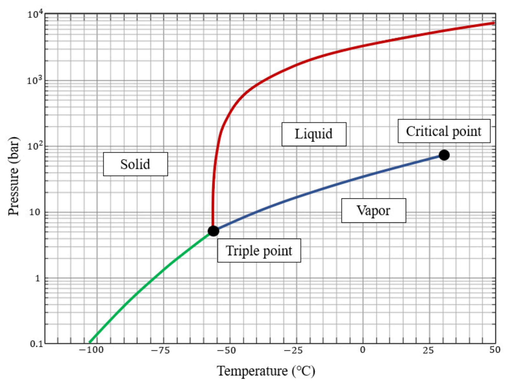
2.1. CO2 Properties and Cargo Tank
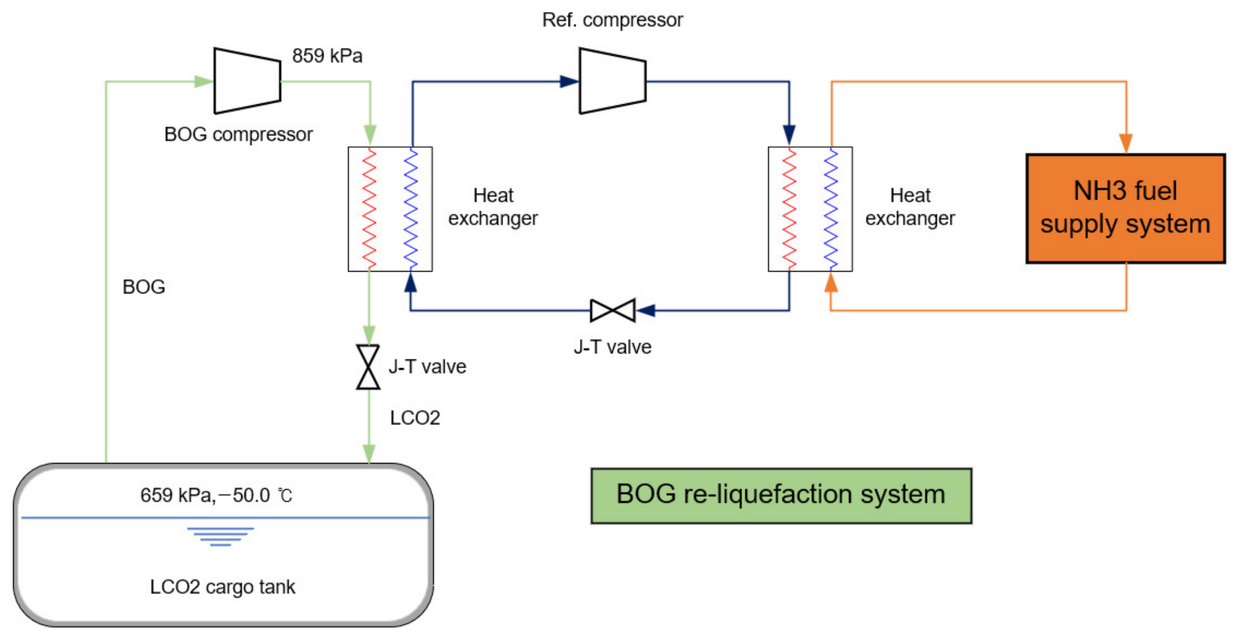
2.2. BOG Re-Liquefaction System
2.3. NH3 Fuel Supply System
3. System Simulation
3.1. Simulation and Validation of Existing Systems
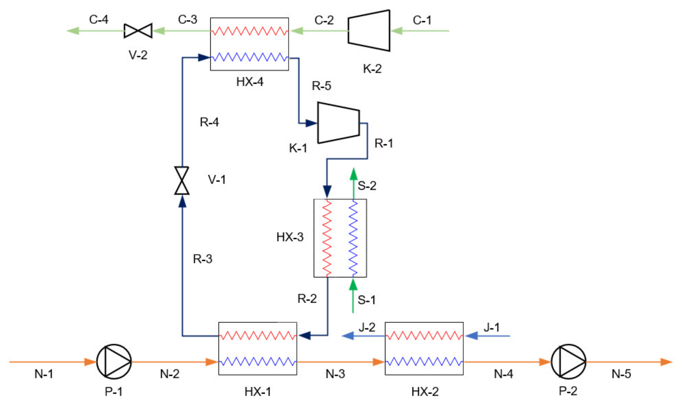
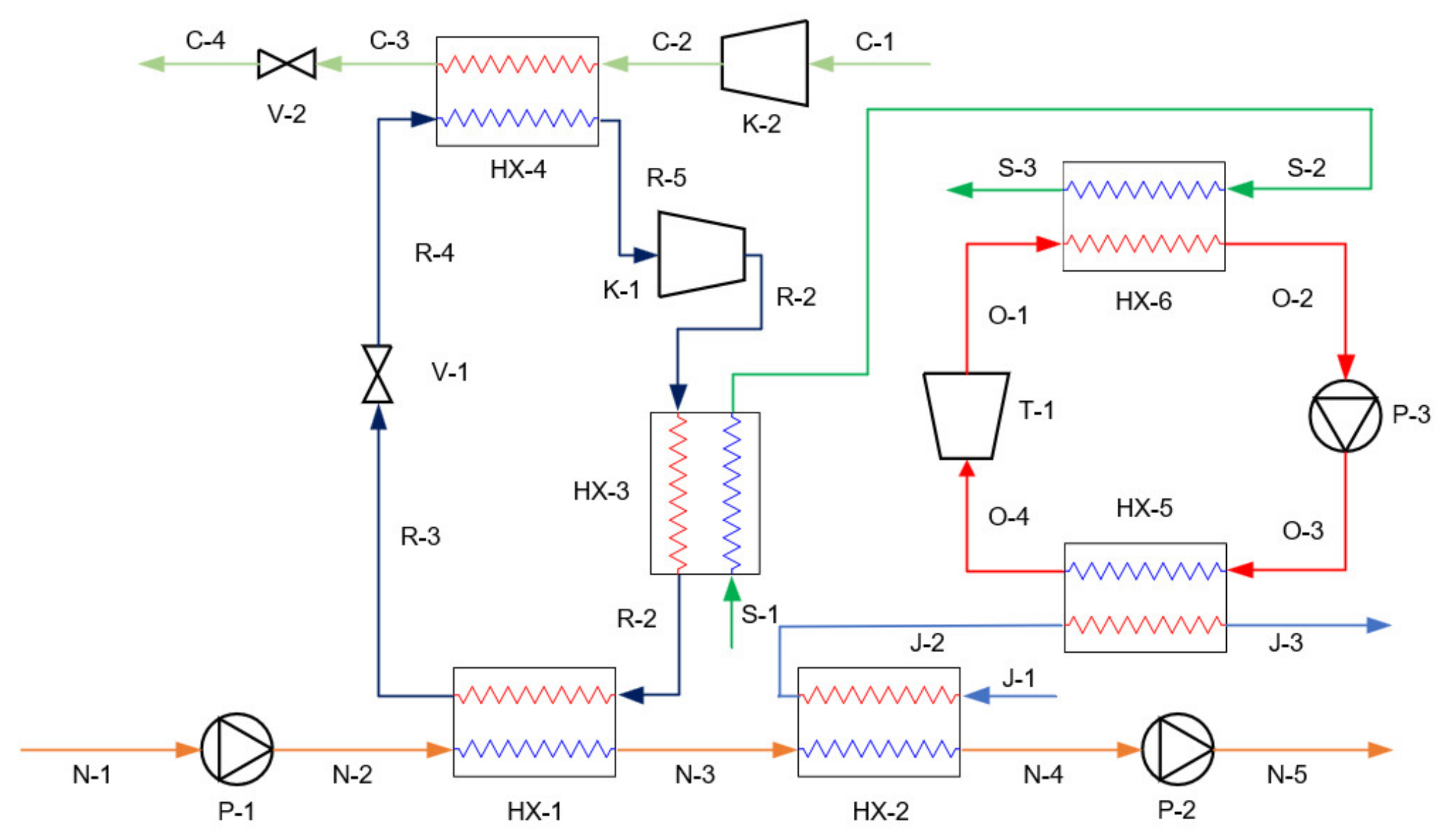
3.2. Simulation of Proposed Systems
4. Analysis Method
4.1. Case Classification
4.2. Independent Variables
- : NH3 fuel mass flow rate, kg/h
- : Ship load, %;
- : Fuel consumption rate, 180 g/(kW∙h);
- : Ship main engine power, 14,500.5 kW;
- : Calorific value of marine diesel oil, 42 MJ/kg;
- : Calorific value of NH3, 18.568 MJ/kg.
4.3. Thermodynamic and Economic Analysis Model
5. Results and Discussion
5.1. Energy Analysis
5.2. Exergy Analysis
5.3. Economic Analysis
6. Conclusions
- Case 2 was simpler than Case 1; however, the energy-analysis results were similar. At a low load and high ambient temperature, the performance of Case 1 was superior to that of Case 2. The and SEC of Case 3 were lower than those of Case 1 by 35.5–45.4 kW and 51.8–171.5, respectively, at a normal load, and 5.1–46.4 kW and 7.4–178.3, respectively, at a low load. Case 3 showed an improved thermodynamic performance owing to the turbine output in the ORC.
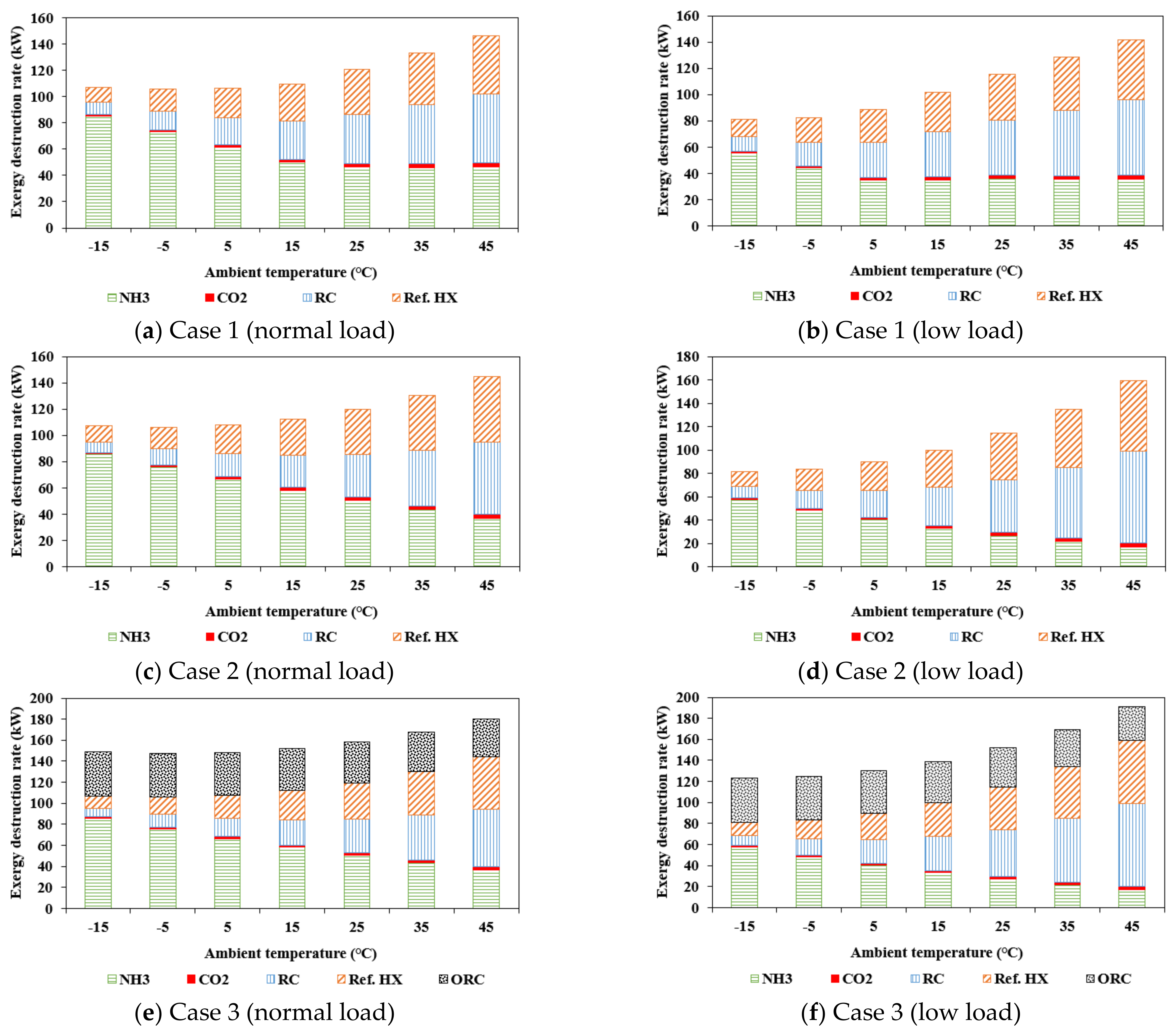
- As a result of the exergy analysis, the results of Cases 1 and 2 were largely the same, except when the ambient temperature was high at a low load, for reasons like those expressed for the energy analysis. Meanwhile, the exergy destruction rate in Case 3 was 33.7–42.4 kW higher at a normal load and 36.1–49.7 kW higher at a low load than Case 1, due to the addition of the ORC. In Case 3, it was important to minimize the ORC exergy destruction rate.
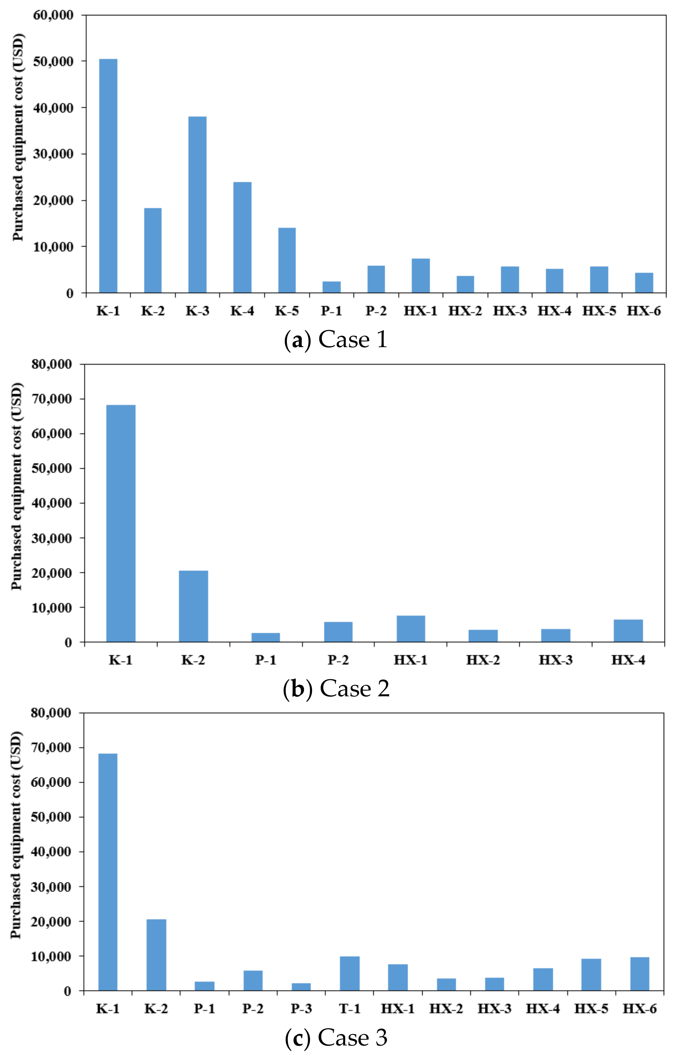
- Case 1 exhibited the highest CAPEX because it required multiple expensive compressors. Instead, the OPEX is lower than that in Case 2, owing to the cascade system. Case 2 had the lowest CAPEX because it used a small number of components, but it used the highest OPEX. Case 3 had a higher CAPEX than Case 2 owing to the ORC, but it had an extremely low OPEX. Cases 2 and 3 proposed in this study can reduce the total annual costs by 17.4% and 20.1%, respectively, compared with Case 1.
Author Contributions
Funding
Institutional Review Board Statement
Informed Consent Statement
Data Availability Statement
Conflicts of Interest
Nomenclature
| Area | Operating period | ||
| BOG | Boil-off gas | NH3 | Ammonia |
| CAPEX | Capital expenditure | ODP | Ozone depletion potential |
| CCUS | Carbon capture utilization and storage | OPEX | Operating expenditure |
| CO2 | Carbon dioxide | ORC | Organic Rankine cycle |
| DC | Direct cost | P | Pump |
| Specific exergy | Pressure | ||
| Exergy destruction rate | PEC | Purchased equipment cost | |
| GWP | Global warming potential | PPTD | Pinch point temperature difference |
| Enthalpy | RC | Refrigerant cycle | |
| H2 | Hydrogen | Ref. | Reference, Refrigerant |
| HP | High pressure | Entropy | |
| HX | Heat exchanger | SEC | Specific energy consumption |
| Interest rate | T | Turbine | |
| IC | Indirect cost | Temperature | |
| J–T | Joule–Thomson | TAC | Total annual cost |
| K | Compressor | TCI | Total capital investment |
| LCO2 | Liquefied carbon dioxide | V | Valve |
| LNG | Liquefied natural gas | VF | Vapor fraction |
| LP | Low pressure | Power | |
| Mass flow rate | |||
| Greeks | |||
| Density | |||
| Subscripts | |||
| 0 | Reference state | In | |
| Critical point | Joule–Thomson | ||
| Cold | Net | ||
| Compressor | Out | ||
| Hot | Pump | ||
| Heat exchanger | Turbine | ||
Appendix A

| Ambient Temperature (°C) | −15 | −5 | 5 | 15 | 25 | 35 | 45 |
|---|---|---|---|---|---|---|---|
| Case 1 (normal load) | |||||||
| K-1 (kW) | 24.49 | 36.64 | 51.64 | 69.90 | 76.28 | 77.38 | 77.20 |
| K-2 (kW) | 3.50 | 4.51 | 5.52 | 6.53 | 6.85 | 6.90 | 6.89 |
| K-3 (kW) | 0.62 | 0.62 | 0.62 | 0.62 | 11.66 | 26.83 | 42.97 |
| K-4 (kW) | 0.21 | 0.21 | 0.21 | 0.21 | 3.97 | 9.13 | 14.62 |
| K-5 (kW) | 0.04 | 0.04 | 0.04 | 0.04 | 0.74 | 1.70 | 2.72 |
| P-1 (kW) | 4.14 | 4.14 | 4.14 | 4.14 | 4.14 | 4.14 | 4.14 |
| P-2 (kW) | 20.44 | 20.44 | 20.44 | 20.44 | 20.44 | 20.44 | 20.44 |
| (kW) | 53.44 | 66.59 | 82.60 | 101.87 | 124.07 | 146.51 | 168.98 |
| SEC (kJ/kg) | 211.39 | 204.90 | 207.95 | 217.01 | 229.05 | 238.66 | 246.28 |
| Case 1 (low load) | |||||||
| K-1 (kW) | 28.69 | 44.38 | 59.71 | 59.36 | 58.06 | 59.08 | 59.10 |
| K-2 (kW) | 3.50 | 4.51 | 5.30 | 5.28 | 5.22 | 5.27 | 5.27 |
| K-3 (kW) | 0.62 | 0.62 | 4.12 | 20.38 | 37.36 | 52.59 | 68.57 |
| K-4 (kW) | 0.21 | 0.21 | 1.40 | 6.93 | 12.71 | 17.89 | 23.33 |
| K-5 (kW) | 0.04 | 0.04 | 0.26 | 1.29 | 2.36 | 3.32 | 4.33 |
| P-1 (kW) | 3.16 | 3.16 | 3.16 | 3.16 | 3.16 | 3.16 | 3.16 |
| P-2 (kW) | 15.63 | 15.63 | 15.63 | 15.63 | 15.63 | 15.63 | 15.63 |
| (kW) | 51.85 | 68.55 | 89.59 | 112.04 | 134.50 | 156.95 | 179.40 |
| SEC (kJ/kg) | 205.13 | 210.92 | 225.55 | 238.67 | 248.31 | 255.66 | 261.47 |
| Case 2 (normal load) | |||||||
| K-1 (kW) | 24.84 | 36.72 | 51.13 | 68.31 | 88.54 | 112.07 | 139.11 |
| K-2 (kW) | 3.54 | 4.55 | 5.56 | 6.57 | 7.58 | 8.59 | 9.60 |
| P-1 (kW) | 4.14 | 4.14 | 4.14 | 4.14 | 4.14 | 4.14 | 4.14 |
| P-2 (kW) | 20.44 | 20.44 | 20.44 | 20.44 | 20.44 | 20.44 | 20.44 |
| (kW) | 52.96 | 65.84 | 81.26 | 99.46 | 120.70 | 145.24 | 173.29 |
| SEC (kJ/kg) | 209.50 | 202.60 | 204.58 | 211.87 | 222.83 | 236.59 | 252.58 |
| Case 2 (low load) | |||||||
| K-1 (kW) | 28.86 | 43.89 | 62.69 | 85.70 | 113.31 | 145.75 | 183.02 |
| K-2 (kW) | 3.54 | 4.55 | 5.56 | 6.57 | 7.58 | 8.59 | 9.60 |
| P-1 (kW) | 3.16 | 3.16 | 3.16 | 3.16 | 3.16 | 3.16 | 3.16 |
| P-2 (kW) | 15.63 | 15.63 | 15.63 | 15.63 | 15.63 | 15.63 | 15.63 |
| (kW) | 51.19 | 67.23 | 87.04 | 111.06 | 139.68 | 173.14 | 211.42 |
| SEC (kJ/kg) | 202.50 | 206.87 | 219.13 | 236.59 | 257.88 | 282.04 | 308.14 |
| Case 3 (normal load) | |||||||
| K-1 (kW) | 24.84 | 36.72 | 51.13 | 68.31 | 88.54 | 112.07 | 139.12 |
| K-2 (kW) | 3.54 | 4.55 | 5.56 | 6.57 | 7.58 | 8.59 | 9.60 |
| P-1 (kW) | 4.14 | 4.14 | 4.14 | 4.14 | 4.14 | 4.14 | 4.14 |
| P-2 (kW) | 20.44 | 20.44 | 20.44 | 20.44 | 20.44 | 20.44 | 20.44 |
| P-3 (kW) | 2.55 | 2.57 | 2.59 | 2.59 | 2.58 | 2.56 | 2.50 |
| T-1 (kW) | 45.41 | 45.59 | 45.53 | 45.24 | 44.66 | 43.75 | 42.36 |
| (kW) | 10.09 | 22.83 | 38.32 | 56.82 | 78.62 | 104.04 | 133.44 |
| SEC (kJ/kg) | 39.90 | 70.24 | 96.48 | 121.04 | 145.15 | 169.48 | 194.49 |
| Case 3 (low load) | |||||||
| K-1 (kW) | 28.86 | 43.89 | 62.69 | 85.70 | 113.31 | 145.76 | 183.02 |
| K-2 (kW) | 3.54 | 4.55 | 5.56 | 6.57 | 7.58 | 8.59 | 9.60 |
| P-1 (kW) | 3.16 | 3.16 | 3.16 | 3.16 | 3.16 | 3.16 | 3.16 |
| P-2 (kW) | 15.63 | 15.63 | 15.63 | 15.63 | 15.63 | 15.63 | 15.63 |
| P-3 (kW) | 2.70 | 2.72 | 2.71 | 2.69 | 2.63 | 2.54 | 2.40 |
| T-1 (kW) | 47.10 | 46.98 | 46.51 | 45.63 | 44.23 | 42.23 | 39.52 |
| (kW) | 6.79 | 22.97 | 43.24 | 68.12 | 98.08 | 133.45 | 174.30 |
| SEC (kJ/kg) | 26.87 | 70.68 | 108.86 | 145.10 | 181.07 | 217.39 | 254.04 |
| Ambient Temperature (°C) | −15 | −5 | 5 | 15 | 25 | 35 | 45 |
|---|---|---|---|---|---|---|---|
| Case 1 (normal load) | |||||||
| (kW) | 4.99 | 7.26 | 9.98 | 13.18 | 14.28 | 14.47 | 14.44 |
| (kW) | 1.09 | 1.40 | 1.71 | 2.03 | 2.12 | 2.14 | 2.14 |
| kW) | 0.10 | 0.10 | 0.10 | 0.10 | 1.92 | 4.43 | 7.09 |
| (kW) | 0.04 | 0.04 | 0.04 | 0.04 | 0.85 | 1.95 | 3.12 |
| (kW) | 0.01 | 0.01 | 0.01 | 0.01 | 0.23 | 0.53 | 0.84 |
| (kW) | 0.85 | 0.85 | 0.85 | 0.85 | 0.85 | 0.85 | 0.85 |
| (kW) | 3.10 | 3.10 | 3.10 | 3.10 | 3.10 | 3.10 | 3.10 |
| (kW) | 5.33 | 8.41 | 12.11 | 16.35 | 17.75 | 17.99 | 17.95 |
| (kW) | 81.18 | 69.37 | 57.72 | 46.25 | 42.74 | 42.17 | 42.25 |
| (kW) | 6.28 | 8.10 | 9.91 | 11.73 | 12.29 | 12.38 | 12.37 |
| (kW) | 0.07 | 0.07 | 0.07 | 0.07 | 1.67 | 3.82 | 6.04 |
| (kW) | 0.05 | 0.05 | 0.05 | 0.05 | 0.86 | 1.98 | 3.18 |
| (kW) | 0.07 | 0.07 | 0.07 | 0.07 | 1.32 | 3.04 | 4.87 |
| (kW) | 3.86 | 6.54 | 10.33 | 15.56 | 17.53 | 17.87 | 17.82 |
| (kW) | 0.06 | 0.07 | 0.09 | 0.10 | 0.11 | 0.11 | 0.11 |
| (kW) | 0.12 | 0.12 | 0.12 | 0.12 | 2.29 | 5.26 | 8.42 |
| (kW) | 0.03 | 0.03 | 0.03 | 0.03 | 0.50 | 1.15 | 1.84 |
| (kW) | 0.00 | 0.00 | 0.00 | 0.00 | 0.01 | 0.03 | 0.04 |
| (kW) | 107.23 | 105.60 | 106.29 | 109.64 | 120.42 | 133.26 | 146.47 |
| Case 1 (low load) | |||||||
| (kW) | 5.68 | 8.49 | 11.16 | 11.10 | 10.87 | 11.05 | 11.05 |
| (kW) | 1.09 | 1.40 | 1.64 | 1.64 | 1.62 | 1.63 | 1.64 |
| (kW) | 0.10 | 0.10 | 0.68 | 3.36 | 6.16 | 8.67 | 11.31 |
| (kW) | 0.04 | 0.04 | 0.30 | 1.48 | 2.71 | 3.81 | 4.97 |
| (kW) | 0.01 | 0.01 | 0.08 | 0.40 | 0.73 | 1.03 | 1.34 |
| (kW) | 0.65 | 0.65 | 0.65 | 0.65 | 0.65 | 0.65 | 0.65 |
| (kW) | 2.37 | 2.37 | 2.37 | 2.37 | 2.37 | 2.37 | 2.37 |
| (kW) | 6.60 | 10.43 | 13.87 | 13.80 | 13.51 | 13.74 | 13.74 |
| (kW) | 52.77 | 41.05 | 32.10 | 32.29 | 32.98 | 32.43 | 32.43 |
| (kW) | 6.28 | 8.10 | 9.51 | 9.48 | 9.37 | 9.46 | 9.46 |
| (kW) | 0.07 | 0.07 | 0.58 | 2.91 | 5.28 | 7.33 | 9.42 |
| (kW) | 0.05 | 0.05 | 0.30 | 1.51 | 2.76 | 3.89 | 5.07 |
| (kW) | 0.07 | 0.07 | 0.47 | 2.31 | 4.24 | 5.97 | 7.78 |
| (kW) | 5.16 | 9.25 | 13.84 | 13.73 | 13.32 | 13.64 | 13.64 |
| (kW) | 0.06 | 0.07 | 0.08 | 0.08 | 0.08 | 0.08 | 0.08 |
| (kW) | 0.12 | 0.12 | 0.81 | 4.00 | 7.32 | 10.31 | 13.44 |
| (kW) | 0.03 | 0.03 | 0.18 | 0.87 | 1.60 | 2.26 | 2.94 |
| (kW) | 0.00 | 0.00 | 0.00 | 0.02 | 0.04 | 0.05 | 0.07 |
| (kW) | 81.14 | 82.30 | 88.64 | 102.00 | 115.63 | 128.38 | 141.41 |
| Case 2 (normal load) | |||||||
| (kW) | 4.75 | 6.80 | 9.19 | 11.94 | 15.07 | 18.61 | 22.59 |
| (kW) | 1.10 | 1.41 | 1.72 | 2.04 | 2.35 | 2.67 | 2.98 |
| (kW) | 0.85 | 0.85 | 0.85 | 0.85 | 0.85 | 0.85 | 0.85 |
| (kW) | 3.10 | 3.10 | 3.10 | 3.10 | 3.10 | 3.10 | 3.10 |
| (kW) | 5.46 | 7.77 | 10.35 | 13.17 | 16.16 | 19.26 | 22.39 |
| (kW) | 81.92 | 71.99 | 62.78 | 54.32 | 46.56 | 39.52 | 33.16 |
| (kW) | 0.26 | 0.64 | 1.37 | 2.57 | 4.36 | 6.87 | 10.20 |
| (kW) | 6.35 | 8.17 | 9.98 | 11.80 | 13.61 | 15.43 | 17.24 |
| (kW) | 3.25 | 5.39 | 8.32 | 12.24 | 17.34 | 23.84 | 31.94 |
| (kW) | 0.06 | 0.07 | 0.09 | 0.10 | 0.12 | 0.14 | 0.15 |
| (kW) | 107.10 | 106.19 | 107.77 | 112.12 | 119.53 | 130.28 | 144.59 |
| Case 2 (low load) | |||||||
| (kW) | 5.33 | 7.80 | 10.76 | 14.23 | 18.28 | 22.92 | 28.17 |
| (kW) | 1.10 | 1.41 | 1.72 | 2.04 | 2.35 | 2.67 | 2.98 |
| (kW) | 0.65 | 0.65 | 0.65 | 0.65 | 0.65 | 0.65 | 0.65 |
| (kW) | 2.37 | 2.37 | 2.37 | 2.37 | 2.37 | 2.37 | 2.37 |
| (kW) | 6.09 | 8.73 | 11.64 | 14.73 | 17.85 | 20.85 | 23.61 |
| (kW) | 54.80 | 45.70 | 37.55 | 30.35 | 24.06 | 18.64 | 14.03 |
| (kW) | 0.52 | 1.35 | 2.86 | 5.26 | 8.74 | 13.40 | 19.29 |
| (kW) | 6.35 | 8.17 | 9.98 | 11.80 | 13.61 | 15.43 | 17.24 |
| (kW) | 4.27 | 7.42 | 11.96 | 18.23 | 26.60 | 37.39 | 50.79 |
| (kW) | 0.06 | 0.07 | 0.09 | 0.10 | 0.12 | 0.14 | 0.15 |
| (kW) | 81.53 | 83.67 | 89.58 | 99.76 | 114.63 | 134.46 | 159.28 |
| Case 3 (normal load) | |||||||
| (kW) | 4.75 | 6.80 | 9.19 | 11.94 | 15.07 | 18.61 | 22.59 |
| (kW) | 1.10 | 1.41 | 1.72 | 2.04 | 2.35 | 2.67 | 2.98 |
| (kW) | 0.85 | 0.85 | 0.85 | 0.85 | 0.85 | 0.85 | 0.85 |
| (kW) | 3.10 | 3.10 | 3.10 | 3.10 | 3.10 | 3.10 | 3.10 |
| (kW) | 0.38 | 0.39 | 0.39 | 0.39 | 0.39 | 0.38 | 0.38 |
| (kW) | 10.79 | 10.84 | 10.82 | 10.75 | 10.62 | 10.40 | 10.07 |
| (kW) | 5.46 | 7.77 | 10.35 | 13.17 | 16.16 | 19.26 | 22.39 |
| (kW) | 81.93 | 71.99 | 62.78 | 54.32 | 46.56 | 39.52 | 33.16 |
| (kW) | 0.26 | 0.64 | 1.37 | 2.57 | 4.36 | 6.87 | 10.20 |
| (kW) | 6.35 | 8.17 | 9.98 | 11.80 | 13.61 | 15.43 | 17.25 |
| (kW) | 16.32 | 16.17 | 15.92 | 15.58 | 15.12 | 14.48 | 13.78 |
| (kW) | 14.12 | 13.92 | 13.63 | 13.23 | 12.73 | 12.11 | 11.35 |
| (kW) | 3.25 | 5.39 | 8.32 | 12.24 | 17.34 | 23.84 | 31.94 |
| (kW) | 0.06 | 0.07 | 0.09 | 0.10 | 0.12 | 0.14 | 0.15 |
| (kW) | 148.72 | 147.50 | 148.52 | 152.08 | 158.40 | 167.65 | 180.19 |
| Case 3 (low load) | |||||||
| (kW) | 5.33 | 7.80 | 10.76 | 14.23 | 18.28 | 22.92 | 28.17 |
| (kW) | 1.10 | 1.41 | 1.72 | 2.04 | 2.35 | 2.67 | 2.98 |
| (kW) | 0.65 | 0.65 | 0.65 | 0.65 | 0.65 | 0.65 | 0.65 |
| (kW) | 2.37 | 2.37 | 2.37 | 2.37 | 2.37 | 2.37 | 2.37 |
| (kW) | 0.41 | 0.41 | 0.41 | 0.40 | 0.40 | 0.38 | 0.36 |
| (kW) | 11.19 | 11.17 | 11.06 | 10.85 | 10.51 | 10.04 | 9.39 |
| (kW) | 6.09 | 8.73 | 11.64 | 14.73 | 17.85 | 20.85 | 23.61 |
| (kW) | 54.80 | 45.70 | 37.55 | 30.35 | 24.06 | 18.64 | 14.03 |
| (kW) | 0.52 | 1.35 | 2.86 | 5.26 | 8.74 | 13.41 | 19.29 |
| (kW) | 6.35 | 8.17 | 9.98 | 11.80 | 13.61 | 15.43 | 17.24 |
| (kW) | 16.37 | 16.12 | 15.71 | 15.14 | 14.37 | 13.41 | 12.32 |
| (kW) | 13.98 | 13.66 | 13.21 | 12.60 | 11.82 | 10.86 | 9.72 |
| (kW) | 4.27 | 7.42 | 11.96 | 18.23 | 26.60 | 37.40 | 50.79 |
| (kW) | 0.06 | 0.07 | 0.09 | 0.10 | 0.12 | 0.14 | 0.15 |
| (kW) | 123.48 | 125.02 | 129.97 | 138.75 | 151.73 | 169.16 | 191.08 |
| Case 1 | Case 2 | Case 3 | |
|---|---|---|---|
| (USD) | 50,467.65 | 68,293.81 | 68,296.55 |
| (USD) | 18,268.18 | 20,445.53 | 20,445.53 |
| (USD) | 37,998.43 | - | - |
| (USD) | 23,898.09 | - | - |
| (USD) | 14,044.76 | - | - |
| (USD) | 2541.52 | 2541.52 | 2541.52 |
| (USD) | 5880.05 | 5880.05 | 5880.05 |
| (USD) | - | - | 2059.05 |
| (USD) | - | - | 9963.49 |
| (USD) | 7446.02 | 7722.63 | 7723.39 |
| (USD) | 3715.08 | 3560.75 | 3560.77 |
| (USD) | 5725.92 | 3719.54 | 3719.60 |
| (USD) | 5193.05 | 6383.53 | 6383.54 |
| (USD) | 5656.06 | - | 9318.87 |
| (USD) | 4287.51 | - | 9738.24 |
| (USD) | 185,122.31 | 11,8547.37 | 149,630.59 |
| (USD) | 299,898.14 | 192,046.74 | 242,401.55 |
| (USD) | 68,976.57 | 44,170.75 | 55,752.36 |
| (USD) | 814,375.61 | 521,504.35 | 658,243.20 |
| (USD/year) | 95,656.25 | 61,255.71 | 77,317.00 |
| (kW) | 168.98 | 173.29 | 133.44 |
| (USD/year) | 88,831.03 | 91,101.90 | 70,151.89 |
| (USD/year) | 184,487.28 | 152,357.60 | 147,468.89 |
References
- Bilgili, L.; Ölçer, A.I. IMO 2023 Strategy-Where Are We and What’s Next? Mar. Policy 2024, 160, 105953. [Google Scholar] [CrossRef]
- Zhang, C.; Zhu, J.; Guo, H.; Xue, S.; Wang, X.; Wang, Z.; Chen, T.; Yang, L.; Zeng, X.; Su, P. Technical Requirements for 2023 IMO GHG Strategy. Sustainability 2024, 16, 2766. [Google Scholar] [CrossRef]
- Zandalinas, S.I.; Fritschi, F.B.; Mittler, R. Global Warming, Climate Change, and Environmental Pollution: Recipe for a Multifactorial Stress Combination Disaster. Trends Plant Sci. 2021, 26, 588–599. [Google Scholar] [CrossRef] [PubMed]
- Bayraktar, M.; Yuksel, O. A Scenario-Based Assessment of the Energy Efficiency Existing Ship Index (EEXI) and Carbon Intensity Indicator (CII) Regulations. Ocean Eng. 2023, 278, 114295. [Google Scholar] [CrossRef]
- Son, H.; Yu, T.; Hwang, J.; Lim, Y. Simulation Methodology for Hydrogen Liquefaction Process Design Considering Hydrogen Characteristics. Int. J. Hydrogen Energy 2022, 47, 25662–25678. [Google Scholar] [CrossRef]
- Kim, J.S.; Kim, D.Y. Energy, Exergy, and Economic (3E) Analysis of SOFC-GT-ORC Hybrid Systems for Ammonia-Fueled Ships. J. Mar. Sci. Eng. 2023, 11, 2126. [Google Scholar] [CrossRef]
- Tapia, J.F.D.; Lee, J.Y.; Ooi, R.E.H.; Foo, D.C.Y.; Tan, R.R. A Review of Optimization and Decision-Making Models for the Planning of CO2 Capture, Utilization and Storage (CCUS) Systems. Sustain. Prod. Consum. 2018, 13, 1–15. [Google Scholar] [CrossRef]
- Bajpai, S.; Shreyash, N.; Singh, S.; Memon, A.R.; Sonker, M.; Tiwary, S.K.; Biswas, S. Opportunities, Challenges and the Way Ahead for Carbon Capture, Utilization and Sequestration (CCUS) by the Hydrocarbon Industry: Towards a Sustainable Future. Energy Rep. 2022, 8, 15595–15616. [Google Scholar] [CrossRef]
- Storrs, K.; Lyhne, I.; Drustrup, R. A Comprehensive Framework for Feasibility of CCUS Deployment: A Meta-Review of Literature on Factors Impacting CCUS Deployment. Int. J. Greenh. Gas Control 2023, 125, 103878. [Google Scholar] [CrossRef]
- Chen, S.; Liu, J.; Zhang, Q.; Teng, F.; McLellan, B.C. A Critical Review on Deployment Planning and Risk Analysis of Carbon Capture, Utilization, and Storage (CCUS) toward Carbon Neutrality. Renew. Sustain. Energy Rev. 2022, 167, 112537. [Google Scholar] [CrossRef]
- Greig, C.; Uden, S. The Value of CCUS in Transitions to Net-Zero Emissions. Electron. J. 2021, 34, 107004. [Google Scholar] [CrossRef]
- Jiang, K.; Ashworth, P.; Zhang, S.; Liang, X.; Sun, Y.; Angus, D. China’s Carbon Capture, Utilization and Storage (CCUS) Policy: A Critical Review. Renew. Sustain. Energy Rev. 2020, 119, 109601. [Google Scholar] [CrossRef]
- Jiang, K.; Ashworth, P. The Development of Carbon Capture Utilization and Storage (CCUS) Research in China: A Bibliometric Perspective. Renew. Sustain. Energy Rev. 2021, 138, 110521. [Google Scholar] [CrossRef]
- Vishal, V.; Chandra, D.; Singh, U.; Verma, Y. Understanding Initial Opportunities and Key Challenges for CCUS Deployment in India at Scale. Resour. Conserv. Recycl. 2021, 175, 105829. [Google Scholar] [CrossRef]
- Bazhenov, S.; Chuboksarov, V.; Maximov, A.; Zhdaneev, O. Technical and Economic Prospects of CCUS Projects in Russia. Sustain. Mater. Technol. 2022, 33, e00452. [Google Scholar] [CrossRef]
- Jeon, S.H.; Kim, M.S. Compressor Selection Methods for Multi-Stage Re-Liquefaction System of Liquefied CO2 Transport Ship for CCS. Appl. Therm. Eng. 2015, 82, 360–367. [Google Scholar] [CrossRef]
- Lu, J.; Li, Y.; Li, B.; Yang, Q.; Deng, F. Research on Re-Liquefaction of Cargo BOG Using Liquid Ammonia Cold Energy on CO2 Transport Ship. Int. J. Greenh. Gas Control 2023, 129, 103994. [Google Scholar] [CrossRef]
- Jeon, S.H.; Kim, M.S. Effects of Impurities on Re-Liquefaction System of Liquefied CO2 Transport Ship for CCS. Int. J. Greenh. Gas. Control 2015, 43, 225–232. [Google Scholar] [CrossRef]
- Jeon, S.H.; Choi, Y.U.; Kim, M.S. Review on Boil-Off Gas (BOG) Re-Liquefaction System of Liquefied CO2 Transport Ship for Carbon Capture and Sequestration (CCS). Int. J. Air-Cond. Refrig. 2016, 24, 1650017. [Google Scholar] [CrossRef]
- Lee, J.; Son, H.; Oh, J.; Yu, T.; Kim, H.; Lim, Y. Advanced Process Design of Subcooling Re-Liquefaction System Considering Storage Pressure for a Liquefied CO2 Carrier. Energy 2024, 293, 130556. [Google Scholar] [CrossRef]
- Lee, Y.; Baek, K.H.; Lee, S.; Cha, K.; Han, C. Design of Boil-off CO2 Re-Liquefaction Processes for a Large-Scale Liquid CO2 Transport Ship. Int. J. Greenh. Gas Control 2017, 67, 93–102. [Google Scholar] [CrossRef]
- Yoo, B.Y. The Development and Comparison of CO2 BOG Re-Liquefaction Processes for LNG Fueled CO2 Carriers. Energy 2017, 127, 186–197. [Google Scholar] [CrossRef]
- Lee, S.G.; Choi, G.B.; Lee, C.J.; Lee, J.M. Optimal Design and Operating Condition of Boil-off CO2 Re-Liquefaction Process, Considering Seawater Temperature Variation and Compressor Discharge Temperature Limit. Chem. Eng. Res. Des. 2017, 124, 29–45. [Google Scholar] [CrossRef]
- Chu, B.; Chang, D.; Chung, H. Optimum Liquefaction Fraction for Boil-off Gas Reliquefaction System of Semi-Pressurized Liquid CO2 Carriers Based on Economic Evaluation. Int. J. Greenh. Gas Control 2012, 10, 46–55. [Google Scholar] [CrossRef]
- Lee, J.; Choi, Y.; Choi, J. Techno-Economic Analysis of NH3 Fuel Supply and Onboard Re-Liquefaction System for an NH3-Fueled Ocean-Going Large Container Ship. J. Mar. Sci. Eng. 2022, 10, 1500. [Google Scholar] [CrossRef]
- Butt, S.S.; Perera, U.A.; Miyazaki, T.; Thu, K.; Higashi, Y. Energy, Exergy and Environmental (3E) Analysis of Low GWP Refrigerants in Cascade Refrigeration System for Low Temperature Applications. Int. J. Refrig. 2024, 160, 373–389. [Google Scholar] [CrossRef]
- Joudi, K.A.; Al-Amir, Q.R. Experimental Assessment of Residential Split Type Air-Conditioning Systems Using Alternative Refrigerants to R-22 at High Ambient Temperatures. Energy Convers. Manag. 2014, 86, 496–506. [Google Scholar] [CrossRef]
- Kim, J.S.; Kim, D.Y.; Kim, Y.T. Experiment on Radial Inflow Turbines and Performance Prediction Using Deep Neural Network for the Organic Rankine Cycle. Appl. Therm. Eng. 2019, 149, 633–643. [Google Scholar] [CrossRef]
- Kim, J.S.; Kim, D.Y.; Kim, Y.T. Thermodynamic Analysis of a Dual Loop Cycle Coupled with a Marine Gas Turbine for Waste Heat Recovery System Using Low Global Warming Potential Working Fluids. J. Mech. Sci. Technol. 2019, 33, 3531–3541. [Google Scholar] [CrossRef]
- Seo, Y.; Huh, C.; Lee, S.; Chang, D. Comparison of CO2 Liquefaction Pressures for Ship-Based Carbon Capture and Storage (CCS) Chain. Int. J. Greenh. Gas Control 2016, 52, 1–12. [Google Scholar] [CrossRef]
- Awoyomi, A.; Patchigolla, K.; Anthony, E.J. CO2/SO2 Emission Reduction in CO2 Shipping Infrastructure. Int. J. Greenh. Gas Control 2019, 88, 57–70. [Google Scholar] [CrossRef]
- Al Baroudi, H.; Awoyomi, A.; Patchigolla, K.; Jonnalagadda, K.; Anthony, E.J. A Review of Large-Scale CO2 Shipping and Marine Emissions Management for Carbon Capture, Utilisation and Storage. Appl. Energy 2021, 287, 116510. [Google Scholar] [CrossRef]
- Bahrami, M.; Pourfayaz, F.; Kasaeian, A. Low Global Warming Potential (GWP) Working Fluids (WFs) for Organic Rankine Cycle (ORC) Applications. Energy Rep. 2022, 8, 2976–2988. [Google Scholar] [CrossRef]
- Kim, J.S.; Kim, D.Y. Energy, Exergy, and Economic (3E) Analysis of Boil-Off Gas Re-Liquefaction Systems Using LNG Cold Energy for LNG-Fueled Ships. J. Mar. Sci. Eng. 2023, 11, 587. [Google Scholar] [CrossRef]
- Strušnik, D.; Avsec, J. Exergoeconomic machine-learning method of integrating a thermochemical Cu-Cl cycle in a multigeneration combined cycle gas turbine for hydrogen production. Int. J. Hydrogen Energy 2022, 47, 17121–17149. [Google Scholar] [CrossRef]
- Tesch, S.; Morosuk, T.; Tsatsaronis, G. Exergetic and Economic Evaluation of Safety-Related Concepts for the Regasification of LNG Integrated into Air Separation Processes. Energy 2017, 141, 2458–2469. [Google Scholar] [CrossRef]
- Cao, X.; Yang, J.; Zhang, Y.; Gao, S.; Bian, J. Process Optimization, Exergy and Economic Analysis of Boil-off Gas Re-Liquefaction Processes for LNG Carriers. Energy 2022, 242, 122947. [Google Scholar] [CrossRef]
- Kim, D.; Hwang, C.; Gundersen, T.; Lim, Y. Process Design and Economic Optimization of Boil-off-Gas Re-Liquefaction Systems for LNG Carriers. Energy 2019, 173, 1119–1129. [Google Scholar] [CrossRef]
- Son, H.; Kim, J.K. Automated Process Design and Integration of Precooling for Energy-Efficient BOG (Boil-off Gas) Liquefaction Processes. Appl. Therm. Eng. 2020, 181, 116014. [Google Scholar] [CrossRef]

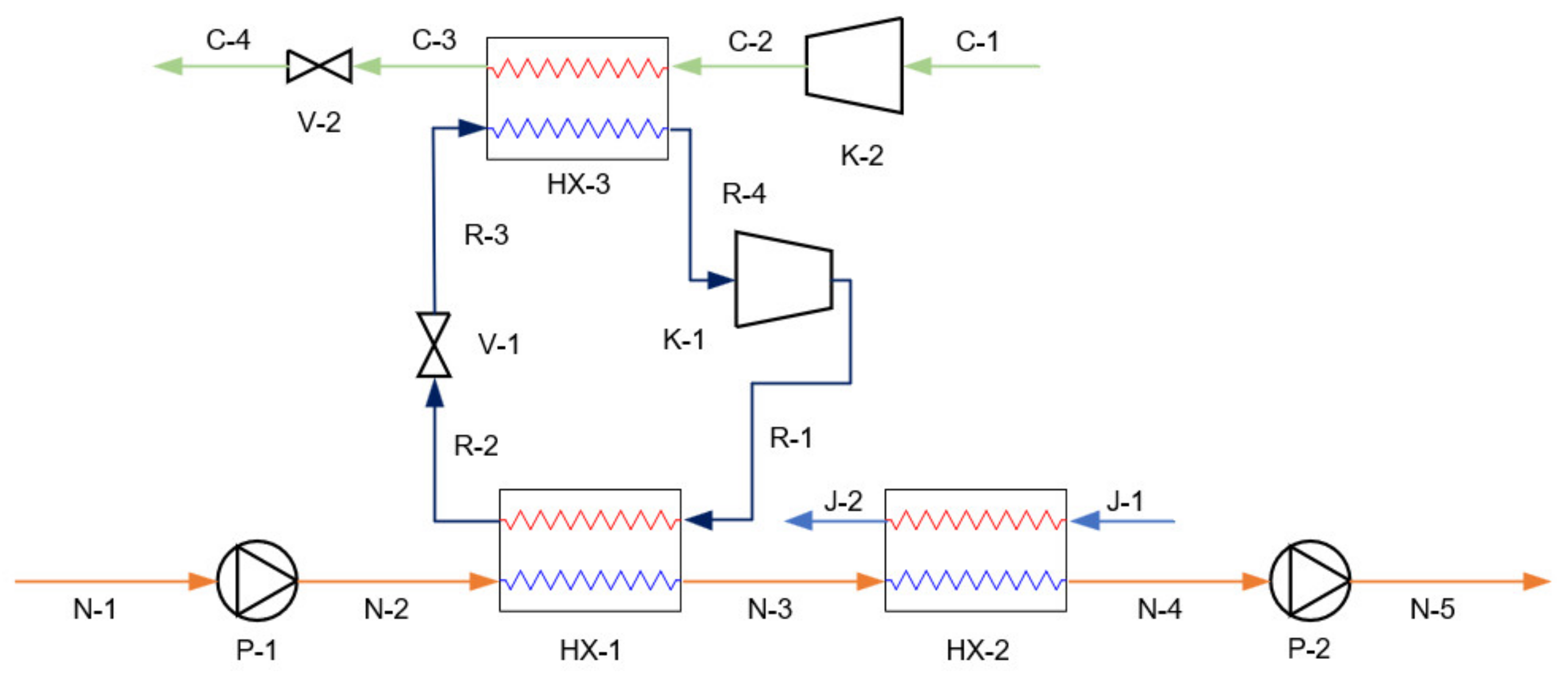


| Stream | Fluid | (°C) | (kPa) | (kg/h) | VF |
|---|---|---|---|---|---|
| N-1 | NH3 | −33.5 | 200 | 5018 | - |
| N-2 | NH3 | - | 1700 | - | - |
| N-4 | NH3 | 40 | - | - | - |
| N-5 | NH3 | - | 8000 | - | - |
| J-1 | H2O | 90 | 200 | 6.3 × 10⁴ | - |
| R-3 | R23 | −55 | - | - | - |
| R-4 | R23 | - | - | - | 1 |
| C-1 | CO2 | −50 | - | 2470 | 1 |
| C-2 | CO2 | - | 859 | - | - |
| C-4 | CO2 | −50 | - | - | - |
| Component | This Study | Lu et al. [17] | Error Rate (%) |
|---|---|---|---|
| K-1 (kW) | 150.3 | 149.0 | 0.87 |
| K-2 (kW) | 9.6 | 9.4 | 2.13 |
| Total (kW) | 159.9 | 158.4 | 0.95 |
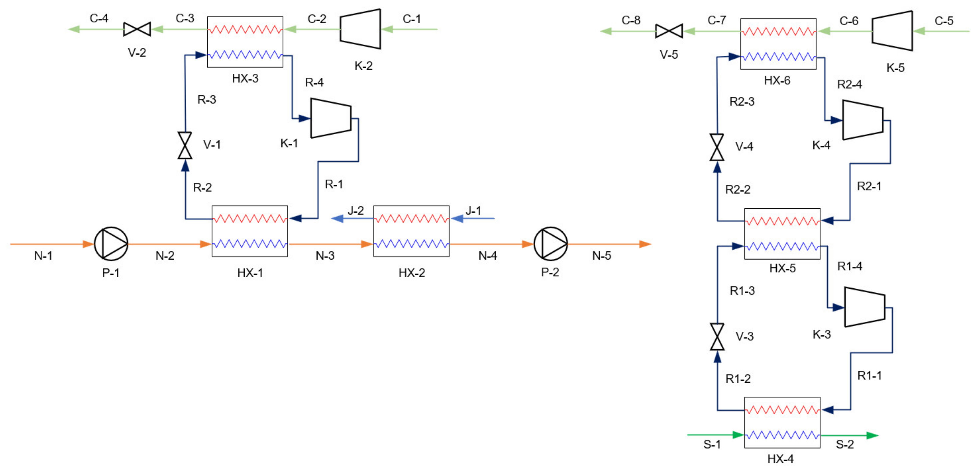
| Stream | Fluid | (°C) | (kPa) | (kg/h) | VF |
|---|---|---|---|---|---|
| S-1 | H2O | 30 | 200 | 9.0 × 10⁴ | - |
| R1-2 | R22 | 40 | - | - | 0 |
| R1-4 | R22 | −30 | - | - | 1 |
| R2-2 | R23 | −25 | - | - | 0 |
| R2-4 | R23 | −55 | - | - | 1 |
| Component | This Study | Lu et al. [17] | Error Rate (%) |
|---|---|---|---|
| K-1 (kW) | 152.0 | 152.2 | 0.13 |
| K-2 (kW) | 51.7 | 51.2 | 0.98 |
| K-3 (kW) | 9.6 | 9.2 | 4.35 |
| Total (kW) | 213.3 | 212.6 | 0.33 |
| Working Fluids | ODP | GWP | (°C) | (kPa) | (kg/m3) | ASHRAE Safety Group | ASHRAE Toxicity |
|---|---|---|---|---|---|---|---|
| R744 | 0 | 1 | 304.19 | 7.38 | 40.8 | A1 | No |
| Stream | Fluid | (°C) | (kPa) | (kg/h) | VF |
|---|---|---|---|---|---|
| N-1 | NH3 | −33.5 | 200 | 5018 | - |
| N-2 | NH3 | - | 1700 | - | - |
| N-4 | NH3 | 40 | - | - | - |
| N-5 | NH3 | - | 8000 | - | - |
| J-1 | H2O | 90 | 200 | 6.3 × 10⁴ | - |
| R-2 | R744 | 35 | - | - | - |
| R-4 | R744 | −55 | - | - | - |
| R-5 | R744 | - | - | - | 1 |
| S-1 | H2O | 30 | 200 | 9.0 × 10⁴ | - |
| C-1 | CO2 | −50 | - | 2470 | 1 |
| C-2 | CO2 | - | 859 | - | - |
| C-4 | CO2 | −50 | - | - | - |
| Stream | Fluid | (°C) | (kPa) | (kg/h) | VF |
|---|---|---|---|---|---|
| O-2 | NH3 | 40 | - | - | 0 |
| O-4 | NH3 | - | - | - | 1 |
| Category. | Equations | Reference |
|---|---|---|
| PEC | ||
| Compressor | Ref. [20] | |
| Pump | Ref. [20] | |
| Turbine | Ref. [34] | |
| Heat exchanger | Ref. [20] | |
| DC | ||
| Equipment installation | Ref. [36] | |
| Piping | ||
| Electrical equipment and materials | ||
| Instrumentation and control | ||
| IC | ||
| Engineering and supervision | Ref. [36] | |
| Construction costs and contractor’s profit | ||
| TCI | Ref. [37] | |
| Stream | Case 1 | Case 2 | Case 3 |
|---|---|---|---|
| NH3 | P-1, HX-2, P-2 | P-1, HX-2, P-2 | P-1, HX-2, P-2 |
| CO2 | K-2, V-2, K-5, V-5 | K-2, V-2 | K-2, V-2 |
| RC | K-1, V-1, K-3, V-3, K-4, V-4 | K-1, V-1 | K-1, V-1 |
| Ref. HX | HX-1, HX-3, HX-4, HX-5, HX-6 | HX-1, HX-3, HX-4 | HX-1, HX-3, HX-4 |
| ORC | - | - | P-3, T-1, HX-5, HX-6 |
| Item | Case 1 | Case 2 | Case 3 |
|---|---|---|---|
| CAPEX (USD/year) | 95,656.253 | 61,255.71 | 77,317.00 |
| OPEX (USD/year) | 88,831.025 | 91,101.90 | 70,151.89 |
| TAC (USD/year) | 184,487.28 | 152,357.60 | 147,468.89 |
Disclaimer/Publisher’s Note: The statements, opinions and data contained in all publications are solely those of the individual author(s) and contributor(s) and not of MDPI and/or the editor(s). MDPI and/or the editor(s) disclaim responsibility for any injury to people or property resulting from any ideas, methods, instructions or products referred to in the content. |
© 2024 by the authors. Licensee MDPI, Basel, Switzerland. This article is an open access article distributed under the terms and conditions of the Creative Commons Attribution (CC BY) license (https://creativecommons.org/licenses/by/4.0/).
Share and Cite
Kim, J.-S.; Kim, D.-Y. Thermodynamic and Economic Analysis of Cargo Boil-Off Gas Re-Liquefaction Systems for Ammonia-Fueled LCO2 Carriers. J. Mar. Sci. Eng. 2024, 12, 1642. https://doi.org/10.3390/jmse12091642
Kim J-S, Kim D-Y. Thermodynamic and Economic Analysis of Cargo Boil-Off Gas Re-Liquefaction Systems for Ammonia-Fueled LCO2 Carriers. Journal of Marine Science and Engineering. 2024; 12(9):1642. https://doi.org/10.3390/jmse12091642
Chicago/Turabian StyleKim, Jun-Seong, and Do-Yeop Kim. 2024. "Thermodynamic and Economic Analysis of Cargo Boil-Off Gas Re-Liquefaction Systems for Ammonia-Fueled LCO2 Carriers" Journal of Marine Science and Engineering 12, no. 9: 1642. https://doi.org/10.3390/jmse12091642