Parametric Estimation of Directional Wave Spectra from Moored FPSO Motion Data Using Optimized Artificial Neural Networks

Abstract

This paper introduces a comprehensive, data-driven framework for parametrically estimating directional ocean wave spectra from numerically simulated FPSO (Floating Production Storage and Offloading) vessel motions. Leveraging a mid-fidelity digital twin of a spread-moored FPSO vessel in the Guyana Sea, this approach integrates a wide range of statistical values calculated from the time histories of vessel responses—displacements, angular velocities, and translational accelerations. Artificial neural networks (ANNs), trained and optimized through hyperparameter tuning and feature selection, are employed to estimate wave parameters including the significant wave height, peak period, main wave direction, enhancement parameter, and directional-spreading factor. A systematic correlation analysis ensures that informative input features are retained, while extensive sensitivity tests confirm that richer input sets notably improve predictive accuracy. In addition, comparisons against other machine learning (ML) methods—such as Support Vector Machines, Random Forest, Gradient Boosting, and Ridge Regression—demonstrate the present ANN model’s superior ability to capture intricate nonlinear interdependencies between vessel motions and environmental conditions.

1. Introduction

Wave measurements often rely on oceanographic instruments such as wave buoys, wave radars, lidars, and cameras. While these methods offer rather accurate measurements, they can be costly to deploy, maintain, and calibrate. Additionally, they may not be suitable for real-time applications or continuous monitoring, limiting their effectiveness in dynamic marine environments. For example, a wave buoy with a single-point mooring system is an expensive device installed in sparse locations. Wave radars and lidars need to cover many grid points to display the wave elevation in space, which requires high computational costs. Cameras are highly influenced by darkness and visibility.

Wave measurement through vessel motions has been proposed as an alternative solution. This method offers the advantage of providing accurate real-time (or near-real-time) wave estimation at a significantly lower cost. Moreover, many structures in the ocean have motion measurement devices on board.

Recently, several studies have proposed machine learning (ML) models for this inverse problem. These methods rely more on data rather than the system’s characteristics. Pioneering studies have explored various aspects of this approach. Firstly, they have considered different input combinations. Reasonably successful wave estimation was achieved using 6 degrees of freedom (6DOF) motions [1,2,3,4,5,6]. Some studies have focused solely on nonplanar motions such as heave, roll, and pitch [7,8,9,10,11]. Despite fewer input parameters, these studies have demonstrated reasonable success in estimating wave conditions, highlighting the critical role of these motions in the inverse problem. Moreover, researchers have attempted various input combinations to enhance ML model performance. Such examples include inputs from 9DOF motions, ship motions with structural responses, a cross-spectrum of ship motion, horizontal/vertical accelerations with pitching motion, heave, surge, and sway displacements, and 6DOF accelerations [12,13,14,15,16,17]. These examples highlight the necessity of selecting appropriate input parameters in inversely estimating wave conditions.

Secondly, for this inverse wave estimation problem, various ML methodologies have been proposed, which include artificial neural networks (ANNs), convolution neural networks (CNNs), recurrent neural networks (RNNs), Random Forest surrogate modeling, and a hybrid approach, i.e., a combination of ML with the wave buoy analogy and an encoder–decoder network [3,4,5,16]. Depending on the system characteristics and data format, the best methodology can be determined. In this regard, comparative analysis among different ML methodologies is crucial for improving estimation performance.

Thirdly, estimating directional waves is also essential for a better understanding of more realistic wave characteristics, yet only a few studies have addressed this issue [6,13,14]. Given the current state of the art, there is a need to further develop approaches and methodologies for directional wave estimation.

This study investigates ANN models to parametrically estimate a near-real-time directional ocean wave spectrum utilizing statistical input data from numerical motion sensors, which can be considered an ideal sensor measurement. The target offshore system was a spread-moored generic FPSO vessel. A coupled time-domain dynamics model with mooring lines and a riser was utilized as a mid-fidelity digital twin of the FPSO system in various sea conditions, capturing its interactions with incoming waves, to furnish motion inputs for the ANNs. The dynamics simulations incorporated diverse wave–current–wind scenarios within feasible parameters. Subsequently, different input variables related to motion signals were integrated and hyperparameter tuning was executed to improve prediction accuracy. Regression plots, case series plots, and multidirectional wave spectra are presented to facilitate visual comparison between the actual and estimated wave parameters, accompanied by systematically presented Root-Mean-Square Error (RMSE) and R-squared values.

There are several unique considerations in the present study. First, unlike prior research endeavors, which often focused on estimating general wave characteristics, this study takes a pioneering step by directly estimating individual wave parameters. These parameters include the significant wave height ($H_s$), wave period ($T_p$), mean wave direction ($\overline{\theta }$), enhancement parameter ($\gamma$), and directional-spreading factor ($s$). By directly estimating each of these parameters, the model provides a comprehensive understanding of directional wave characteristics, allowing more effective decision-making in various applications. Second, through utilizing numerical motion sensor signals, this research explores various combinations of input variables, i.e., employing a total of 119 statistical variables obtained from vessel responses—comprising 6DOF displacements, 3DOF angular velocities, and 3DOF translational accelerations. This input feature extends beyond the narrow set of traditional input variables used by other researchers. Such a rich input domain as the one used in this study enables the model to uncover nuanced, complex relationships that are often overlooked in simpler frameworks. Systematic feature correlation and sensitivity analyses guide the selection and weighting of these input variables, enhancing both model robustness and interpretability. To support our hypothesis of improved performance through the adding of more correlated input variables, the case is compared to those with reduced input parameters. Third, to further demonstrate the advantages of the proposed method, a rigorous comparative analysis is presented against various ML techniques—Support Vector Machines, Random Forest, Gradient Boosting, and Ridge Regression. These comparisons reveal the optimized ANN models to be particularly adept at capturing intricate data patterns linking vessel motions to individual wave parameters. Finally, the model training and validation process relies on a synthetic dataset generated through completely random sampling across a range of realistic environmental conditions. Incorporating actual statistical distributions of waves, winds, and currents ensures that the ANN models can effectively handle environmental variability and maintain their integrity under entirely random conditions. The resulting models thus exhibit improved robustness and adaptability, generalizing more effectively to a wide array of real-world operational scenarios. A detailed analysis and discussion of the findings substantiate the proposed concept.

2. Data Collection

2.1. Numerical FPSO Model

A generic FPSO unit with a length of 310 m was chosen as a numerical model in a water depth of 1500 m, as depicted in Figure 1. The details of the FPSO unit are presented in

Table 1. Principal particulars of the FPSO unit.

Parameter	Symbol	Unit	Value
Length between perpendicular	Lpp	m	310
Breadth	B	m	47.17
Depth	H	m	28.04
Draft	d	m	18.90
Displacement	-	MT	240,869
Center of gravity above base	KG	m	13.30
Roll radius of gyration at CG	Rxx	m	14.77
Pitch radius of gyration at CG	Ryy	m	77.47
Yaw radius of gyration at CG	Rzz	m	79.30
Heave natural period	Tn3	s	14.62
Roll natural period	Tn4	s	12.88
Pitch natural period	Tn5	s	11.79

. The FPSO unit has 12 spread mooring lines and one steel catenary riser.

Table 2. Specification of the mooring lines.

Parameter	Unit	Segment 1 (Chain)	Segment 2 (Polyester)	Segment 3 (Chain)
Length	m	120.0	2290	90.0
Diameter	cm	9.52	16.0	9.52
Dry weight	N/m	1856	168.7	1856
Wet weight	N/m	1615	44.1	1615
Axial stiffness	kN	912,081	186,825	912,081
Minimum breaking load	kN	7553	7429	7553

shows the mooring line particulars [18,19]. There are four mooring groups, and each mooring group has 3 semi-taut chain–polyester–chain mooring lines. The central mooring line of each group is 45° from the longitudinal plane of the FPSO unit, and the three adjacent lines have 5° intervals. The total length of each mooring line from the fairlead point to the anchor point is 2500 m with a corresponding horizontal distance of 1950 m.

The time-domain simulations of the moored FPSO unit were conducted by OrcaFlex [20] to collect big datasets for the training and testing of ML. First, the 3D radiation/diffraction problem was solved in the frequency domain to evaluate the added mass, radiation damping, and first- and second-order wave loads [21]. The hydrodynamic coefficients were then used in the corresponding Cummins equation for the simulation of the FPSO system in the time domain, where nonlinear viscous drag forces were also included. The mooring lines and the riser were modeled from a line model based on the lumped-mass method. A line consists of a certain number of nodes featuring finite lumped-mass elements. Linear axial, bending, and torsional springs were placed to connect lumped nodes while all the physical properties of the lumped node were considered. The element numbers for the mooring lines and the riser were 250 and 280, respectively, which were enough to present their dynamic behaviors.

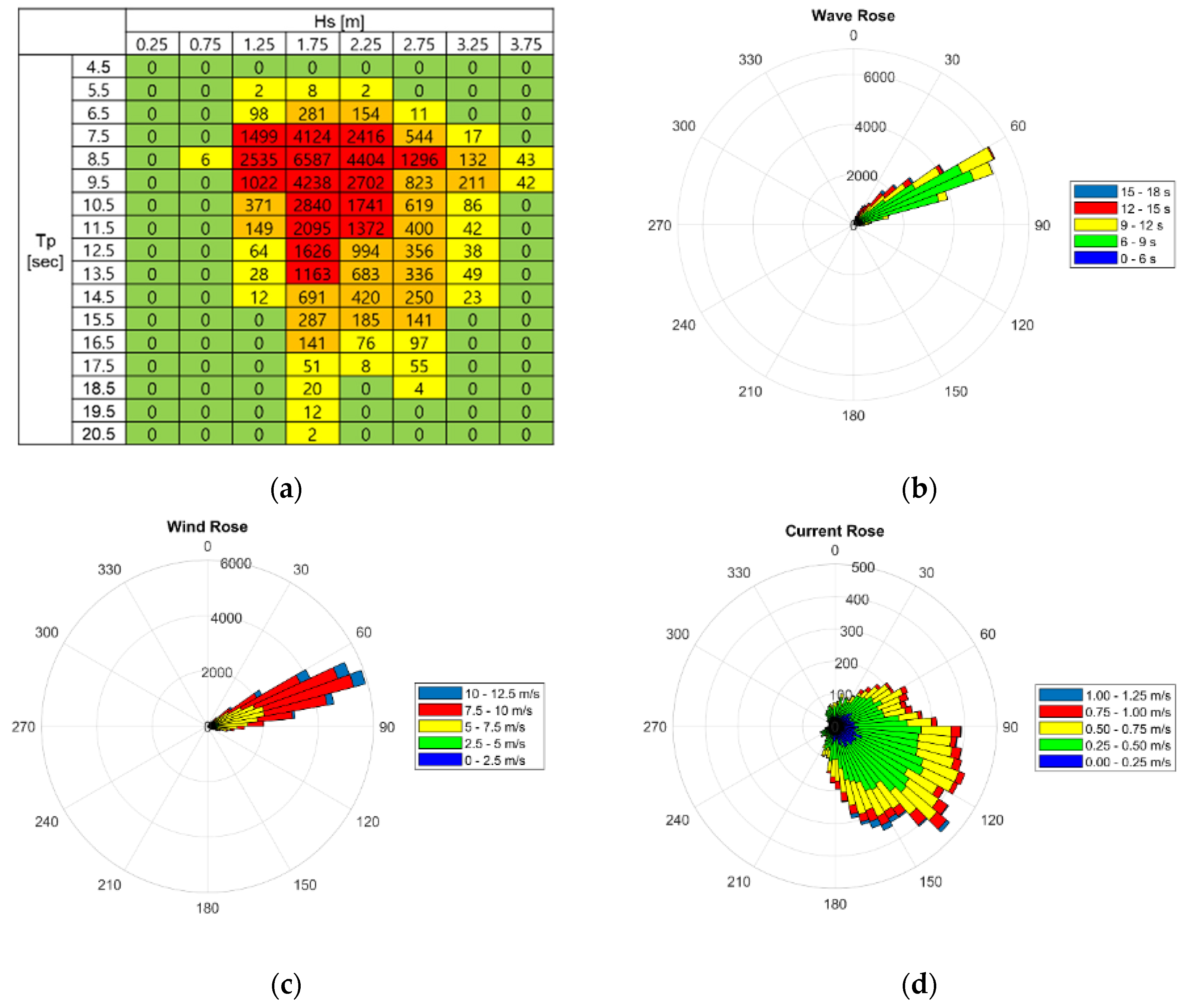
2.2. Environmental Conditions

Data on environmental conditions were collected at −56 degrees east (longitude) and 10 degrees north (latitude) in South America’s North Sea, close to one of the locations where an FPSO unit is currently operated. The 4-year wave and wind statistical data from the years 2018 to 2021 were obtained from ERA5 (fifth-generation ECMWF atmospheric reanalysis of the global climate) [22]. Surface current velocity data from the years 2012 to 2015 were obtained from HYCOM (Hybrid Coordinate Ocean Model) [23]. ERA5 and HYCOM provide publicly available metocean data. Note that these datasets in different years were based on data availability. Figure 2 shows wave–wind–current rose plots in the chosen location. The most probable wave conditions were 1 m < significant wave height ($H_s$) < 3 m and 6 s < peak period ($T_p$) < 14 s. The maximum wind velocity was 12.67 m/s from the east–northeast direction, while the maximum surface current velocity was 1.25 m/s toward the northwest direction. Wind, wave, and current directions were in the ranges of 30–90°, 30–90°, and 30–180°, respectively. The $H_s$ in this location is relatively lower than in other locations such as the Gulf of Mexico. Milder sea conditions may present difficulty in the application of traditional methods, such as the Kalman filter and Bayesian optimization, since the vessels tend to respond less in low sea states. In this sense, the ML model was adopted here, and its robustness is extensively investigated in the following sections.

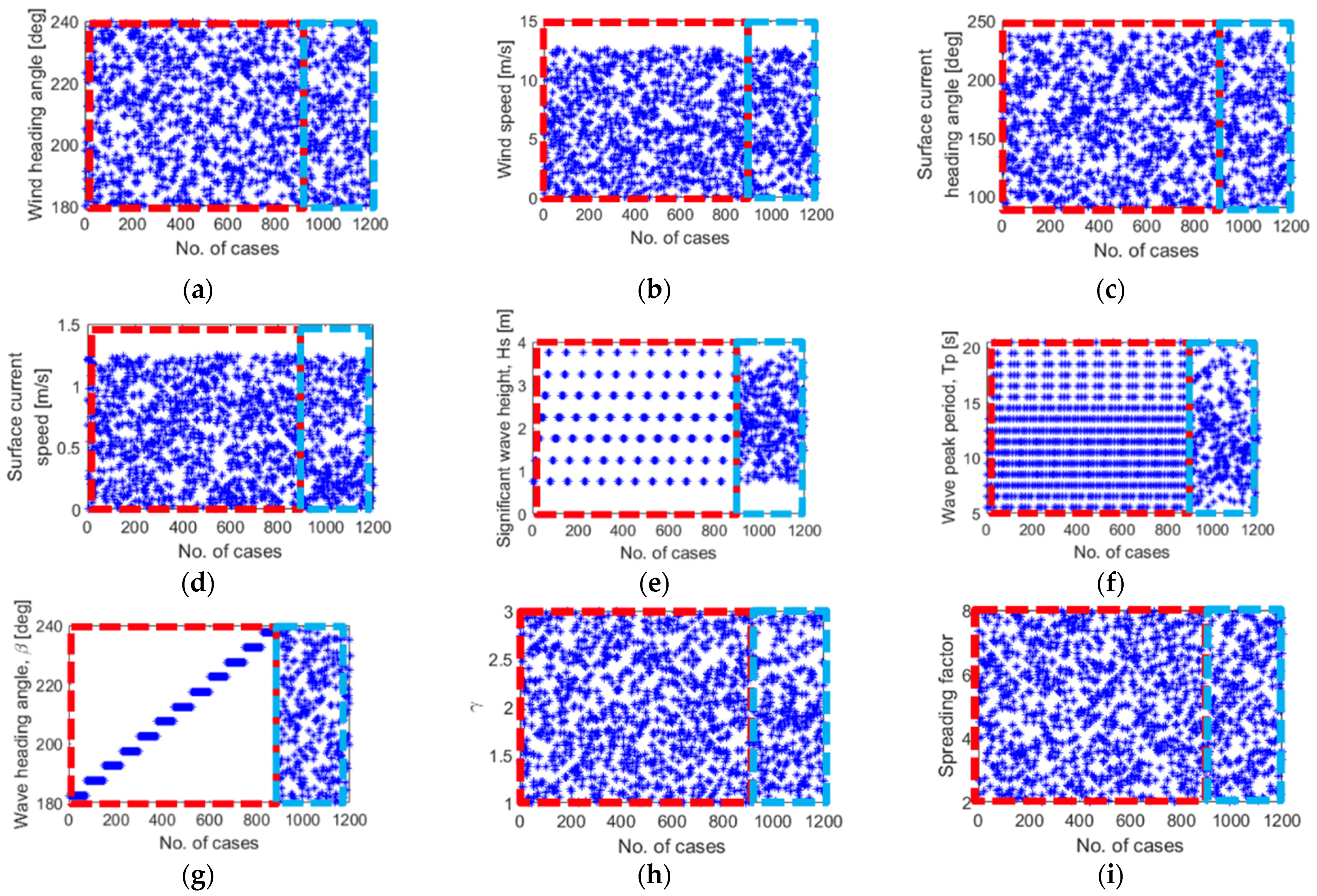
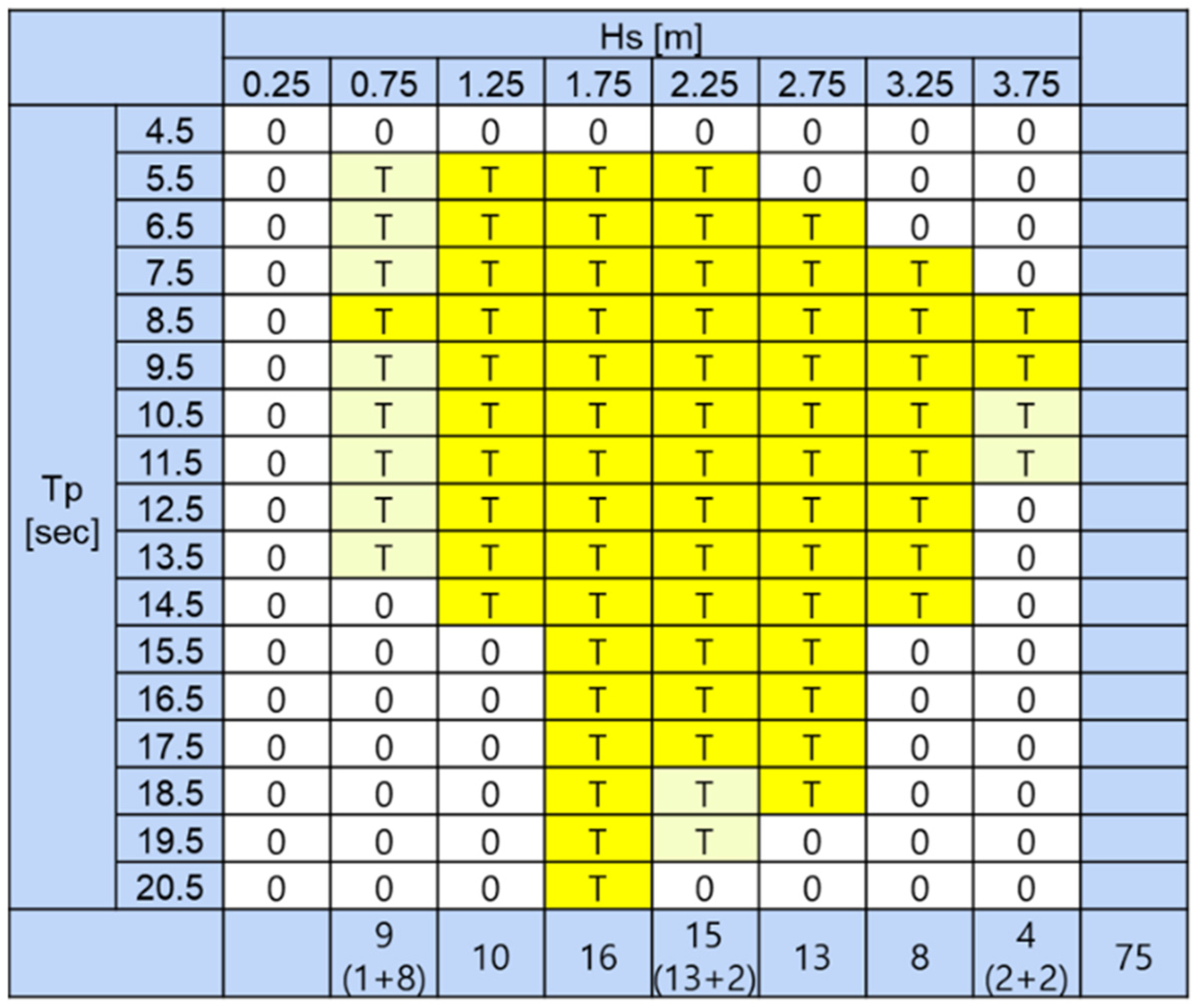
2.3. Synthetic Data Generation

A total of 1200 simulations were conducted for the training and testing of the ML model. Figure 3 illustrates the environmental conditions and the corresponding training and test datasets. The JONSWAP wave spectrum with typical cosine-powered directional spreading was employed for multidirectional wave generations. A multidirectional wave can be expressed as the product of a unidirectional wave spectrum $S_J\left(\omega \right)$ and a directional-spreading function $D\left(\theta \right)$:

$$S\left(\omega ,\theta \right)=S_J\left(\omega \right)· D\left(\theta \right)$$

(1)

where $S_J\left(\omega \right)$ denotes the JONSWAP wave spectrum evaluated at an angular frequency $\omega$, and $D\left(\theta \right)$ is the directional-spreading function centered about the main wave direction ${\theta }_0$. In this study, the directional spreading is based on a “${\cos }^{2s}$” form:

$$D\left(\theta \right)=2^{2s-1}{\displaystyle \frac{\Gamma \left(s+1\right)\Gamma \left(s\right)}{\pi \Gamma \left(2s\right)}}{\left[\cos \left(\theta -{\theta }_0\right)\right]}^{2s}$$

(2)

where $s$ is the spreading factor (or spreading exponent) controlling how wave energy is distributed across directions. The normalization factor $K\left(s\right)=2^{2s-1}\Gamma \left(s+1\right)\Gamma \left(s\right)/\pi \Gamma \left(2s\right)$ ensures that ${{\displaystyle \int }}_{{\theta }_0-\pi }^{{\theta }_0+\pi }D\left(\theta \right)d\theta =1$. The wave spectrum is based on a JONSWAP formulation that modifies a Pierson–Moskowitz baseline:

$$S_J\left(\omega \right)=A_{\gamma }{\displaystyle \frac{5}{16}}{H}_s^2{\omega }_p^4{\omega }^{-5}\exp \left[-{\displaystyle \frac{5}{4}}{\left({\displaystyle \frac{\omega }{{\omega }_p}}\right)}^{-4}\right]{\gamma }^{\exp \left(-{\left(\omega -{\omega }_p\right)}^2/\left(2{\sigma }^2{{\omega }_p}^2\right)\right)}$$

(3)

where $A_{\gamma }$ is a normalizing factor depending on $\gamma$, $\sigma$ is a parameter related to the spectral shape, and ${\omega }_p$ is peak wave frequency.

For training datasets, based on the wave scatter diagram shown in Figure 4, 75 typical combinations of $H_s$ and $T_p$ were selected. In addition, twelve wave directions were considered within the range of the measured wave direction. Therefore, nine hundred simulation examples in total were used for training purposes (i.e., 75 wave conditions times 12 wave directions). Additionally, the enhancement parameter and the spreading factor were randomly chosen within the ranges of 1–3 and 2–8, respectively. The surface current/wind velocities were randomly assigned from the minimal and maximal values measured during the observation time. The corresponding wind/current directions were randomly assigned within the range of measurements. Next, a total of three hundred wave, wind, and current conditions were taken into account as the test datasets; each condition was randomly chosen within the respective training dataset’s range, as shown in the blue box in Figure 3.

2.4. FPSO Motions from Numerical Simulation

Under the configured environmental conditions, 1 h simulation for each case was conducted with a time step of 0.25 s. Figure 5 presents representative 6 DOF motion signals for $H_s$ = 2.25 m, $T_p$ = 15.5 s, and $\overline{\theta }$ = 47.5° with other randomly selected variables (wind velocity = 0.60 m/s; current velocity = 0.95 m/s; wind direction = 56°; and surface current direction = 85°). As shown in Figure 5, nonplanar motions (i.e., heave, roll, and pitch motions) oscillate in the wave-frequency range while planar motions (i.e., surge, sway, and yaw motions) have much larger low-frequency components than wave-frequency components. The low-frequency surge–sway–yaw motions result from the second-order slowly varying wave excitations. When compared to other motion modes, surge and sway movements are significant. These kinds of behaviors have been reported as typical motion trends of FPSO vessels [24,25]. The 6DOF motions, 3DOF angular velocities, and 3DOF translational accelerations from the numerical simulations were then used as input variables in the ML model to inversely estimate the target wave parameters. In particular, several statistical values were calculated and extracted from the 1 h motion time histories to be used as input variables for ML, which include the standard deviations, the second spectral moments (m2), the fourth spectral moments (m4), the mean up-crossing periods ($T_z$), the mean crest periods ($T_c$), etc. The details of the statistical variables are presented in Section 3.2.

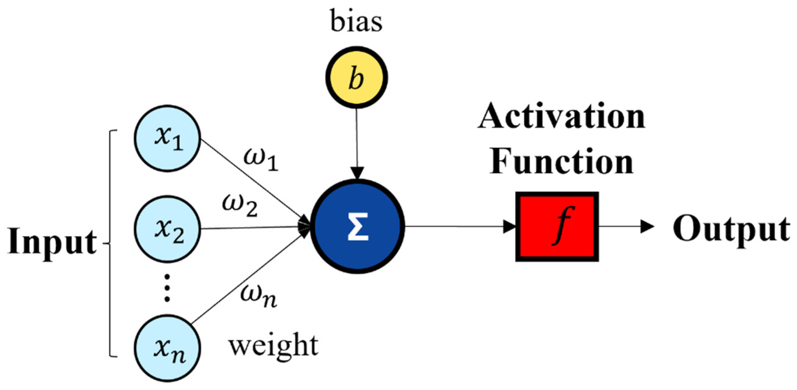
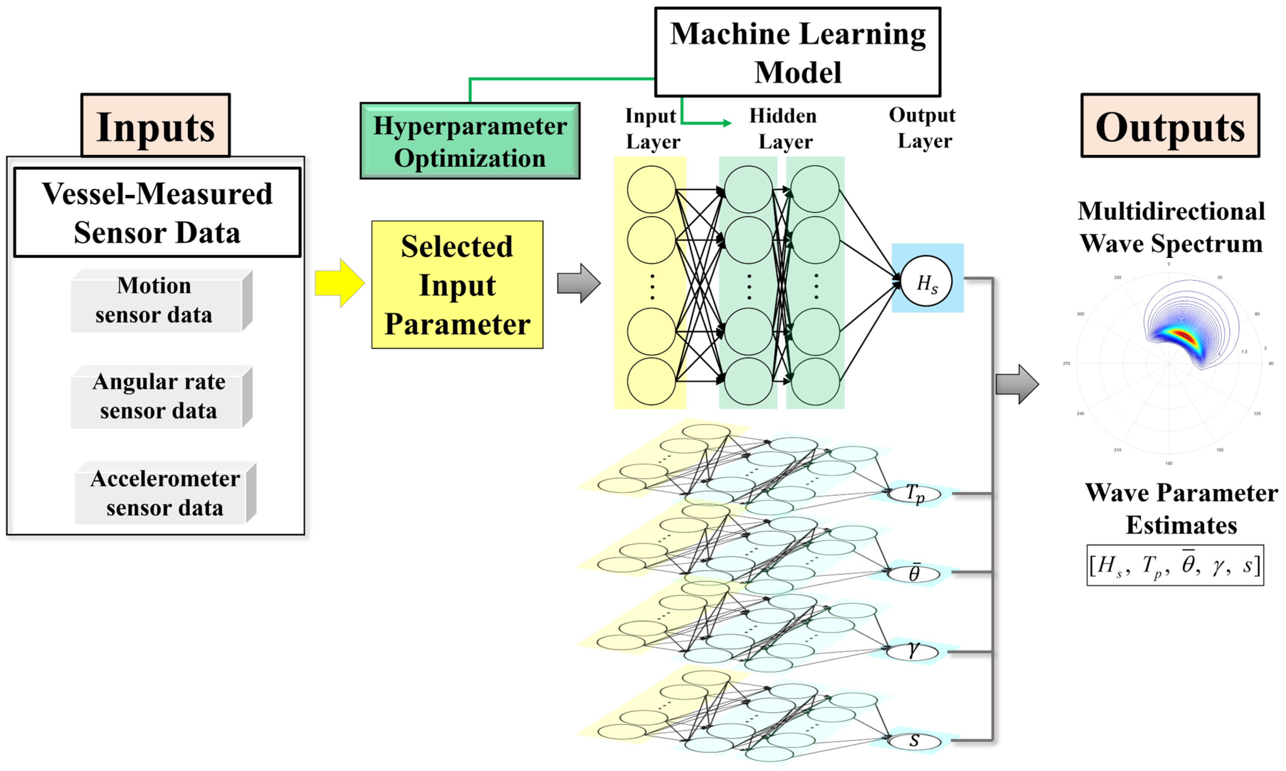
3. ANN for Inverse Wave Estimation from Motion Sensor

The inverse estimation of incoming waves from motion measurements is a typical inverse problem, for which there exists no unique solution. Also, it is impossible to directly (or theoretically) solve the relevant physics. In this regard, we employed the ANN method to solve this problem. The Kalman filter can also be used to solve the inverse problem with a proper physics model [26,27], while ANNs other than PINNs (physics-informed NNs) do not need any physics model. While an ANN can effectively approximate the nonlinear relationship between motion signals and wave parameters, its limitations include the requirement of a large, high-quality training dataset, potential overfitting, and a lack of direct physical interpretability. An ANN is a mathematical model designed to mimic an organism’s ability to learn and understand the correlation between input and output without explicit relational expressions. They comprise an input layer for receiving data, an output layer for producing results, and one or more hidden layers connecting them. Each layer comprises a certain number of nodes. In ANNs, learning involves determining the weights and biases in each layer to minimize the disparity between the final estimated output value by ML and the actual value. The learning process mechanism is illustrated in Figure 6. It earns the term “feedforward” because it traverses through an intermediate layer housing the activation function $f\left(x\right)$ as it progresses from the input nodes $x$ to the ultimate output $y$. Initially, the weights ${\omega }_n$, input $x$, and bias $b$ assess the weighted sum of inputs $x$. To better include the nonlinear relationship between inputs and outputs, the activation function is subsequently included to determine whether external connections perceive this neuron as activated or not. The network eventually generates the predicted value $y$, while the network error is calculated as the difference between the correct output $y$ and the predicted value $y$.

3.1. Applied Methodology

ANNs were trained using the Keras library [28] with TensorFlow as the backend [29], operating on a PC with 16.0 GB RAM, a 2.30 GHz processor, and a 64-bit operating system. The training process for the neural network (NN) model took less than 2 min, which was dependent on the size of the NN model. The network was trained for a maximum of 100 epochs, with each hyperparameter configuration repeated 11 times to alleviate the effects of random weight initialization. The mean squared error (MSE) was used as the loss function, and a learning rate of 0.001 for optimizers such as Adam or Nadam was adopted. EarlyStopping was instantiated to monitor the training loss with a patience of two epochs, though it was not applied as a callback in the final training loop. Instead, whenever an iteration achieved a higher $R^2$ on the test set, the model was saved and considered a representative trained model. Figure 7 illustrates the ANN for inverse wave estimation. The five wave parameters ($H_s$, $T_p$, $\overline{\theta }$, $\gamma$, and s) were estimated and assigned to the output layer. Note that the five NN models were constructed to separately estimate the five wave parameters so that the NNs could best tune the weights for each wave parameter without losing accuracy. This means that only one output among the five wave parameters was assigned to the output layer by the NN model. For comparison, multiple-output cases were also tested, and their performances were worse than in the present approach. The input layer comprised statistical values from 6DOF motions and velocities/accelerations (i.e., 6DOF displacements (subscript 1–6), 3DOF (roll–pitch–yaw; subscript 7, 8, 9) angular velocities, and 3DOF (surge–sway–heave; subscript 10, 11, 12) translational accelerations). These motion signals are directly measurable using a DGPS, inclinometer, angular rate sensor, and accelerometer. The combination of statistical parameters for each NN model was determined by sensitivity tests with respect to different levels of correlations, referred to as the threshold in later sections. Each NN model was tuned through a hyperparameter selection process, such as through the number of neurons and layers as well as the types of activation function and optimizer, which is detailed in Section 3.3.

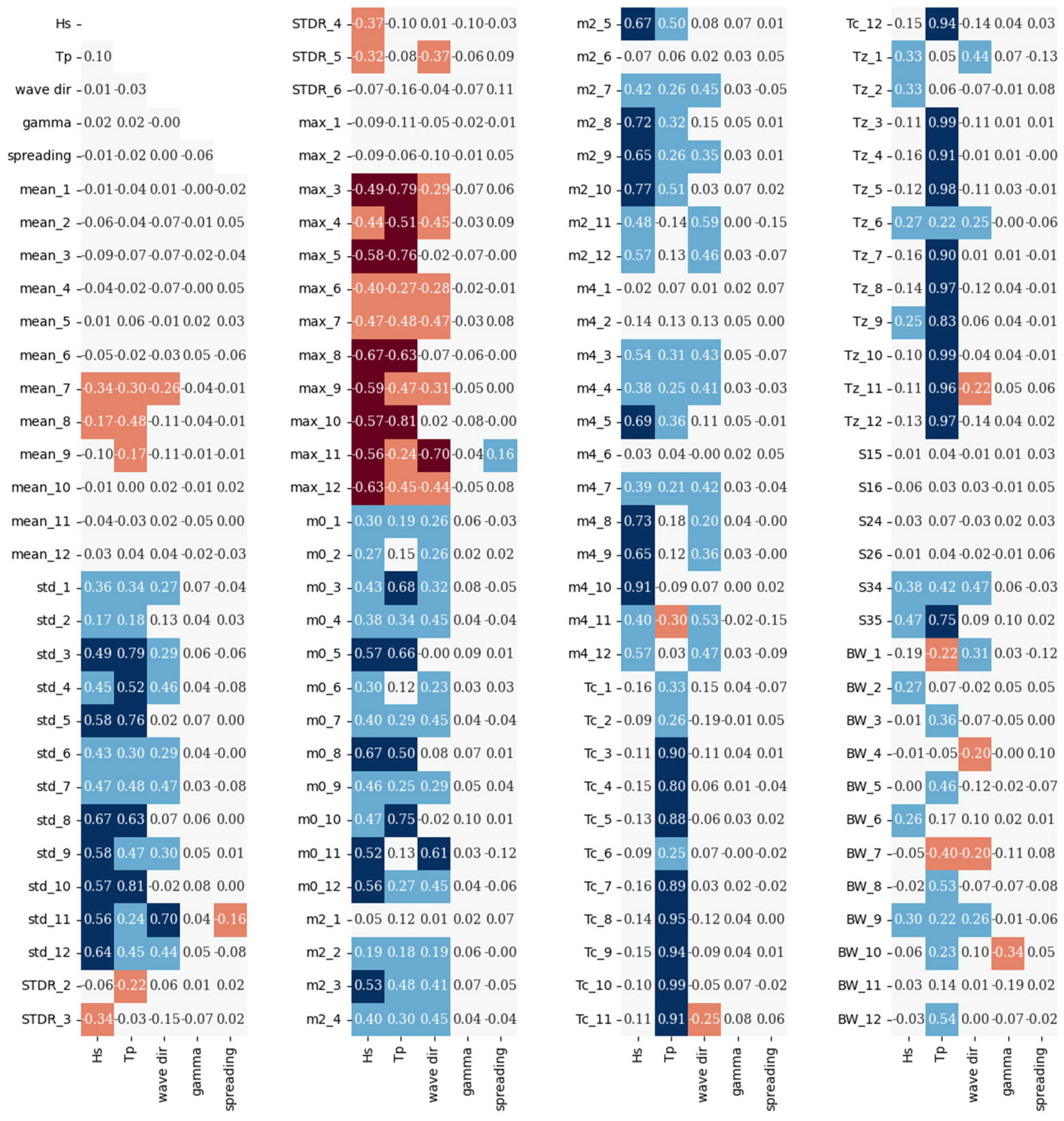
3.2. Feature Correlation

This section analyzes how strongly input and output are correlated. Correlation has been widely used to find a relationship between two or more variables in ML studies [30,31,32]. To obtain the correlation between multiple variables, the matrix data structure, called a correlation heatmap, was identified. By obtaining the correlation heatmap, we could identify the most correlated combinations of inputs. The correlation coefficients have values anywhere between −1 and 1.

In this regard, many potential statistical variables were selected and assessed, as listed in Figure 8, illustrating the feature correlation heatmap. Means, standard deviations (std), relative standard deviations (STDR), one-tenth max values (max), zeroth/second/fourth spectral moments (m0, m2, m4), zero-crossing and crest periods ($T_z$ and $T_c$), cross-correlations (S), and spectral bandwidths (BW) were selected in this study. In Figure 8, cell color coding makes it simple to detect correlations between variables immediately. The blue color (value: 1) means a positive correlation, and the red color (value: −1) means a negative correlation. Also, the white color means no correlation between the two variables. The results show that the mean values of the 1 h FPSO motions do not correlate with the wave parameter, as expected, but the standard deviations of the hourly FPSO motions are related to the wave parameters, especially to $H_s$ and $T_p$. The motion of an FPSO unit is influenced by ocean waves, and thus, the relative standard deviation of the motions can capture important information about the characteristics of the waves that affect the vessel. In this regard, relative standard deviation was computed and used as input for the ML model. It was calculated by dividing the standard deviations of sway–heave–roll–pitch–yaw displacements by the standard deviation of surge displacement. The one-tenth max value is proven to be an important input variable with a remarkably high correlation with $H_s$, $T_p$, and $\overline{\theta }$ through the correlation heatmap. Furthermore, the absolute maximum cross-correlation values (marked as S15, S16, S24, S26, S34, and S35 for the modes of surge and pitch, surge and yaw, sway and roll, sway and yaw, heave and roll, and heave and pitch) were utilized as input to improve the accuracy of estimating wave parameters. The zeroth, second, and fourth moments of the spectrum were the other key variables. The zeroth moment of the spectrum refers to the total energy contained within a specific frequency range. The second moment of the spectrum provides information about the average frequency content or spectral centroid. This moment indicates where the majority of energy or power is concentrated within the frequency range of interest. The fourth moment of the spectrum is related to the spectral spread or width. It provides information about the distribution of energy across different frequencies within the spectrum. These variables mostly have a high correlation with $H_s$, $T_p$, and $\overline{\theta }$. Some of the mean crest period, mean up-crossing period, and bandwidth values have high correlations with $T_p$, and the bandwidth of surge acceleration (BW_10) has the highest correlation of 0.34 with the enhancement parameter among all input variables. The standard deviation of sway acceleration has the highest correlation with the wave main direction $\overline{\theta }$. However, none of the variables exhibit a correlation exceeding 0.2 with the spreading factor, making the estimation of the spreading factor challenging.

Figure 9 shows a series of $H_s$ for all cases. In parallel, the correlations of other variables with $H_s$ are also given. m4_10 shows the highest correlation with $H_s$ at 0.91, followed by m4_11 with a correlation of 0.40. $T_c$_11 has the lowest correlation among the 119 statistical values. These variables are depicted in a series graph. The pattern of m4_10 (the 4th spectral moment of the 10th mode = surge acceleration) is similar to the trend and cycle of $H_s$, showing a high correlation of 0.91, while the crest periods of the 11th mode (heave acceleration), $T_c$_11, have a similar cycle, but the trend does not match with $H_s$, resulting in a low correlation of 0.11. Figure 9 indicates that the selection of proper statistical variables as inputs is an important task in improving the performance of the present ML model.

3.3. Hyperparameter Selection

A parametric study is crucial in determining the optimal hyperparameters for hidden layers. The hidden layer hyperparameters, such as the number of hidden layers, the number of neurons in each hidden layer, the activation functions, and the optimizer, influence the network’s performance and ability to learn complex patterns from data. By systematically varying the values of these hyperparameters, we can identify the settings that yield the best results. The numbers of hidden layers and neurons per layer determine the model’s capacity to capture complex patterns in the data. Activation functions introduce nonlinearities into the network, enabling it to learn nonlinear relationships in the data. Different activation functions have different properties and affect the network’s behavior. Moreover, the choice of an optimizer and its hyperparameters can significantly impact the performance and convergence of an NN. Different optimizers have different strengths and weaknesses, and their effectiveness can vary depending on the specific task and dataset.

Grid search was adopted in this study, which is a methodical approach to hyperparameter optimization in ML, systematically evaluating combinations of hyperparameters to enhance model performance. The chosen hyperparameters included the number of neurons per layer, from 12 to 256, allowing the exploration of varying network complexities. Layer sizes from 1 to 5 were explored to enable the assessment of different network depths. The activation functions considered were Rectified Linear Unit (ReLU) and Exponential Linear Unit (ELU), which are commonly used in neural networks. Optimizers such as Adam, Nadam, and RMSprop were examined for their impact on model training. Grid search streamlines hyperparameter tuning by automating the exploration process, leading to more effective and efficient model optimization. However, even with the same hyperparameters set, the initial random weights assigned to the networks may be different, which may lead to different training processes and results. In this regard, running was repeated eleven times for each hyperparameter case. The MSE was used as the loss function, and the model with the highest $R^2$ was defined as the best model. The MSE measures the average squared difference between the predicted values from the model and the actual observed values. It is represented as

$$MSE={\displaystyle \frac{1}{n}}{{\displaystyle \sum }}_{i=1}^n{\left(y_i-{\widehat{y}}_i\right)}^2$$

(4)

where n is the number of observations, $y_i$ is the actual observed value, and ${\widehat{y}}_i$ is the predicted value for observation $i$. $R^2$ is a measure of how well the independent variables explain the variability in the dependent variable in a regression model. It ranges from 0 to 1, where 1 indicates that the independent variables perfectly explain the variability in the dependent variable. Mathematically, it is defined using the ratio of the sums:

$$R^2=1-{\displaystyle \frac{S{S}_{res}}{S{S}_{tot}}}$$

(5)

where $S{S}_{res}$ is the sum of squares of residuals (errors), and $S{S}_{tot}$ is the total sum of squares. The best hyperparameters for estimating wave parameters obtained through grid search are given in

Table 3. Selected hyperparameters for each wave parameter (The results are based on the best-performed ones listed in Table 4).

Parameter	${\mathit{H}}_{\mathit{s}}$	${\mathit{T}}_{\mathit{p}}$	$\overline{\mathit{\theta }}$	$\mathit{\gamma }$	$\mathit{s}$
Number of layers	4	4	3	1	3
Number of neurons	128	256	256	128	64
Activation function	ELU	ELU	ELU	ELU	ELU
Optimizer	Nadam	Adam	Adam	Adam	Nadam

.

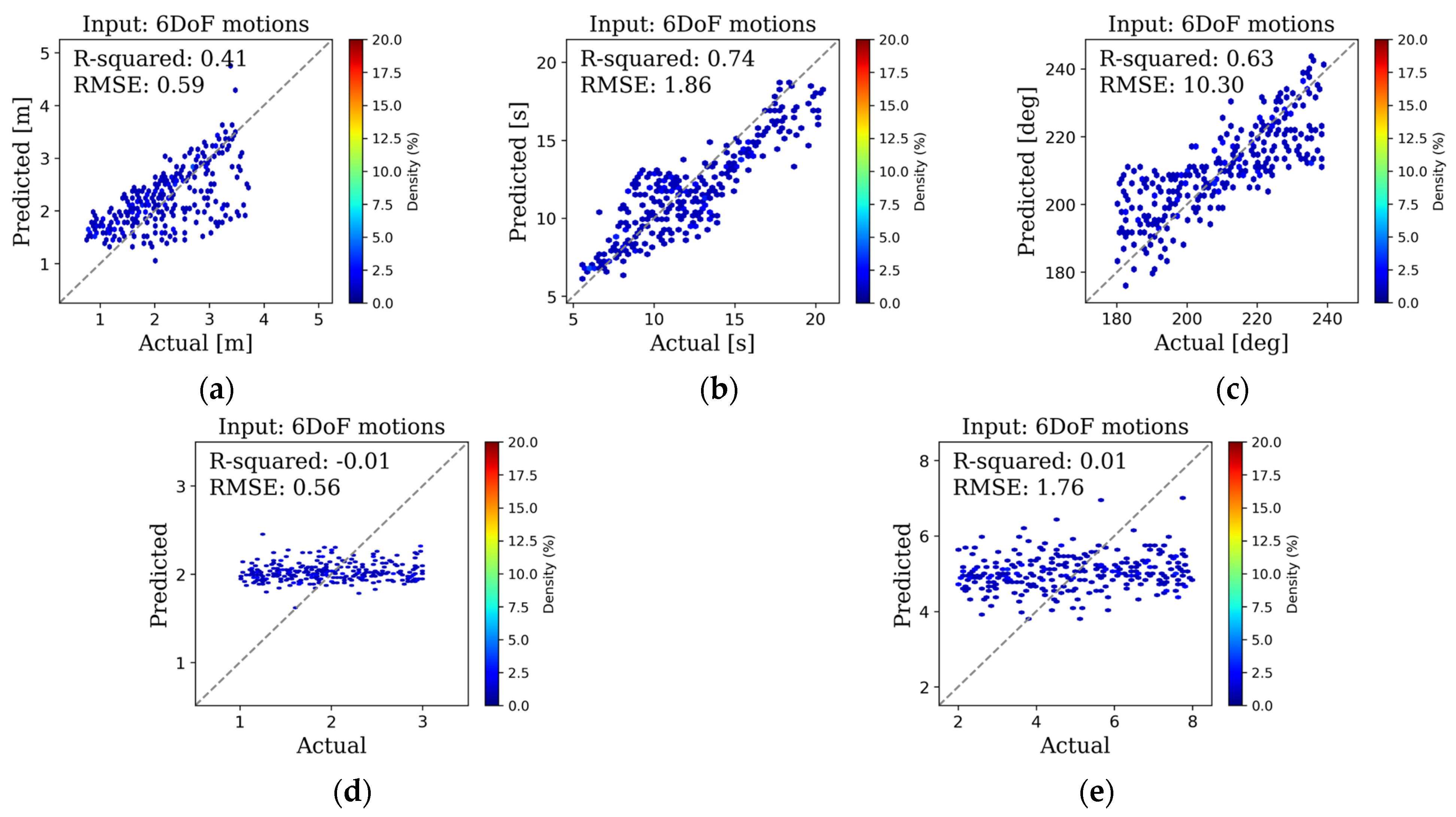
4. Results and Discussion

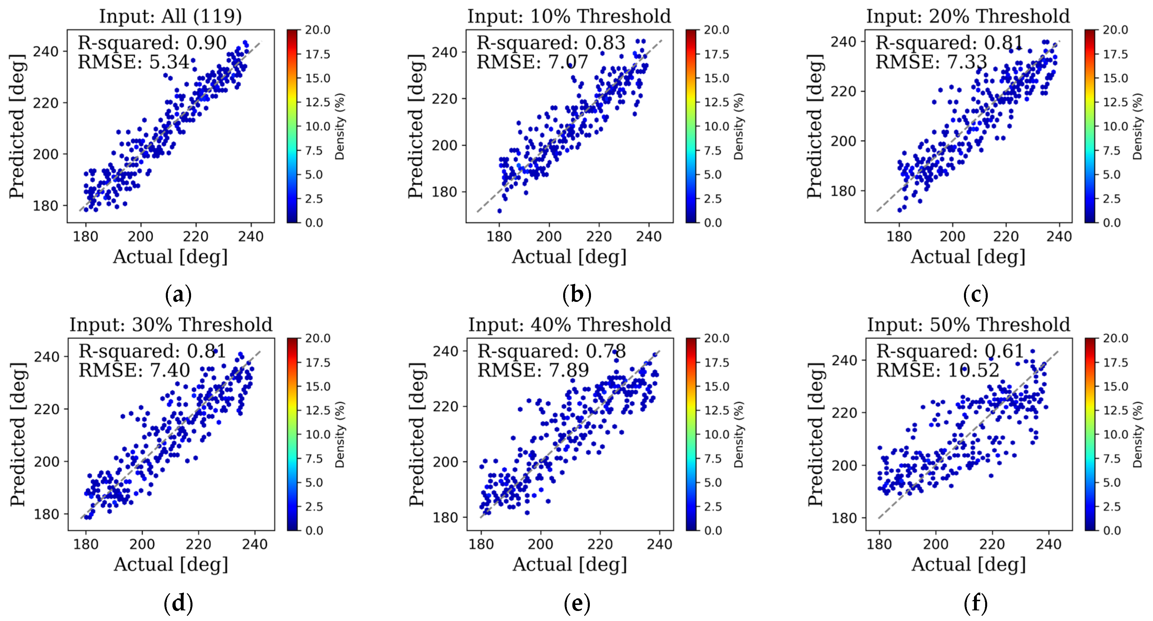
4.1. Sensitivity Analysis with Respect to Input

This section discusses sensitivity with respect to input selection to build a high-performing NN. When displacements and accelerations are compared, accelerations typically show high-frequency signals, while opposite trends are shown for displacements. So, the inclusion of acceleration and angular velocity can help to improve the estimation performance in a wider frequency range. In addition, there are several well-correlated input variables for a specific output. Then, the selection of highly correlated inputs for a specific output can help in the better tuning of the NN model. These interesting topics are presented and discussed here.

Firstly, Figure 10 shows the regression plots, with the mean and standard deviation of 6DOF motions serving as inputs (a total of 12 inputs). It is well known that an FPSO unit’s mean position is mostly governed by the mean current and wind values, while the dynamic wind and wave values play an important role in low-frequency and wave-frequency dynamic behaviors. This means that the mean and standard deviation of motions can be reasonable input parameters to provide the expected output, by eliminating current and wind effects from the mean values and correlating wave parameters with standard deviations. As shown in Figure 10, the $R^2$ of significant wave height is 0.41, denoting that approximately 41% of the variability in $H_s$ can be explained by the mean and standard deviation of 6DOF motions. This $R^2$ indicates a moderate level of performance and underscores the complexity in accurately estimating $H_s$ solely based on these input variables. In contrast, the $R^2$ of wave peak period is notably higher at 0.74, and the $R^2$ of wave main direction stands at 0.63, reflecting a moderate-to-high level of accuracy. This result indicates a significant relationship between the input variables and the estimated wave peak period and wave main direction. On the other hand, the enhancement parameter and spreading factor are hard to estimate using the given inputs, with an $R^2$ of almost zero, indicating the need for additional input variables to improve the predictive capabilities of the model.

Secondly, Figure 11 shows the regression plots with additional motion-based statistical values as inputs. Compared with Figure 10, the means and standard deviations of surge–sway–heave translational accelerations and roll–pitch–yaw angular velocities are additionally considered (a total of 24 inputs). For convenience, we call this the 12DOF case. The Inertial Measurement Unit (IMU) can provide this additional data. Combining these sensors provides richer data for the better facilitation of the ANN through training to estimate wave variables more accurately. As previously mentioned, the acceleration and angular velocity signals tend to be more pronounced in the high- and mid-frequency ranges, which can lead to improved estimation across various frequency ranges. As proven in Figure 11, the additional 6DOFs significantly improve the overall performance of $H_s$, $T_p$, and $\overline{\theta }$ estimations, with $R^2$ values of 0.79, 0.89, and 0.80, respectively, compared to Figure 10, in which only 6DOF motions are used as input. However, the $R^2$ values of the enhancement parameter and spreading factor are still close to zero. Therefore, we attempted to address this problem by incorporating more statistical variables.

Next, to further improve the accuracy of inverse wave estimation, various statistical variables from 12DOFs were introduced, as described in Section 3.2. In addition, the analysis explored the impact of variable thresholds on predicting wave parameters. For example, the 10% threshold stands for the input variables with a 10% or higher correlation. By including variable thresholds in ANN training, we could identify the optimal combination of input variables. Figure 12 represents the regression plots of $\overline{\theta }$ at varying thresholds. While using a larger number of variables (up to 119) does improve estimation accuracy, leading to a high $R^2$ value of 0.9 for $\overline{\theta }$, this scenario could represent a comprehensive but less practical data-rich approach. In other words, compared with the cases with a smaller number of inputs (mean and standard deviation of each mode) as presented in Figure 10 and Figure 11, the present case with additional statistical parameters as input improves accuracy, although significant data processing efforts are inevitable. Still, in the case of $\overline{\theta }$, using the mean and standard deviation as input results in acceptable accuracy from a practical point of view. On the one hand, even when fewer variables are selected under stricter thresholds, accuracy does diminish but is still acceptable for practical applications. As the threshold increases, both the number of input variables and the $R^2$ value decrease, suggesting a weakened relationship between the selected variables and the target parameter. With a threshold of 50%, only five variables are selected as input for $\overline{\theta }$, resulting in a lower $R^2$ value of 0.61.

Table 4 summarizes the $R^2$ values of respective wave parameters as a function of threshold. As all variables are used as input, sometimes, less important variables are assigned high weights, and conversely, important variables are assigned low weights, which can lead to deficient performance [33]. To avoid this, training is performed repeatedly, more than ten times, for the same hyperparameter case. Repeated training runs confirm that more input variables consistently lead to improved model accuracy, but in practical terms, one might strike a balance between the number of variables and the achievable accuracy. For instance, while an extremely high $R^2$ (close to 1 for $T_p$) is attainable with a full set of inputs, selecting a smaller, more feasible subset of well-correlated variables could still provide robust estimates with less complexity and uncertainty in data acquisition.

Through this comprehensive assessment, it can be concluded that having various statistical parameters improves accuracy to some degree. Again, there should be a trade-off between accuracy and the practicality of collecting and processing input variables. Therefore, depending on the needs and accuracy level, different input variables can be implemented, and the present study can provide insights on the selection of input variables.

Table 4. The number of input variables and the resulting estimation accuracy with a correlation threshold from 10% to 50% (N is the number of variables).

		${\mathit{H}}_{\mathit{s}}$	${\mathit{T}}_{\mathit{p}}$	$\overline{\mathit{\theta }}$	$\mathit{\gamma }$	$\mathit{s}$
All	N	119	119	119	119	119
	$R^2$	0.99	1.00	0.90	0.48	0.39
Threshold 10	N	85	94	68	4	8
	$R^2$	0.96	0.99	0.83	0.26	0.03
Threshold 20	N	64	76	46	1
	$R^2$	0.95	0.98	0.81	0.14
Threshold 30	N	58	56	30
	$R^2$	0.95	0.99	0.81
Threshold 40	N	42	48	24
	$R^2$	0.93	0.99	0.78
Threshold 50	N	28	35	5
	$R^2$	0.95	0.99	0.61

Table 4. The number of input variables and the resulting estimation accuracy with a correlation threshold from 10% to 50% (N is the number of variables).

		${\mathit{H}}_{\mathit{s}}$	${\mathit{T}}_{\mathit{p}}$	$\overline{\mathit{\theta }}$	$\mathit{\gamma }$	$\mathit{s}$
All	N	119	119	119	119	119
	$R^2$	0.99	1.00	0.90	0.48	0.39
Threshold 10	N	85	94	68	4	8
	$R^2$	0.96	0.99	0.83	0.26	0.03
Threshold 20	N	64	76	46	1
	$R^2$	0.95	0.98	0.81	0.14
Threshold 30	N	58	56	30
	$R^2$	0.95	0.99	0.81
Threshold 40	N	42	48	24
	$R^2$	0.93	0.99	0.78
Threshold 50	N	28	35	5
	$R^2$	0.95	0.99	0.61

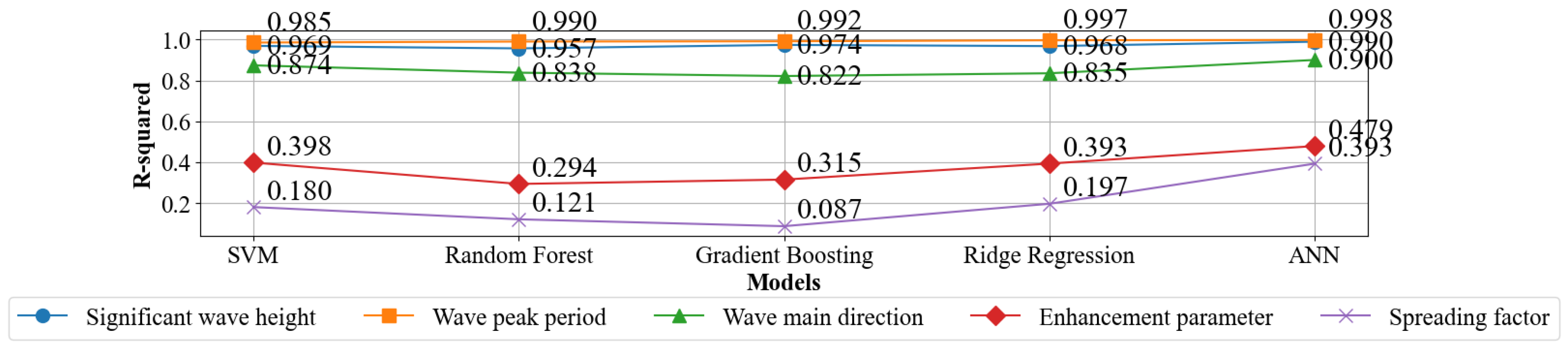
4.2. Comparison with Other ML Methods

This section compares wave estimation results acquired from variable ML methods. As mentioned in the Introduction, each ML method can have pros and cons, so selecting an appropriate ML algorithm is an important task. Support Vector Machines (SVMs), Random Forest (RF), Gradient Boosting (GB), and Ridge Regression were additionally taken into consideration. SVM is a supervised learning method used for classification and regression tasks, optimizing a hyperplane to separate classes in high-dimensional space. RF constructs multiple decision trees and aggregates their predictions to improve generalization and mitigate overfitting. GB iteratively combines weak learners, minimizing the loss function by focusing on previous mistakes. Ridge Regression adds a penalty term to the linear regression objective to mitigate overfitting, which is particularly effective when dealing with multicollinearity. Each technique offers unique advantages and can be chosen based on factors like data complexity, interpretability, and computational resources.

Figure 13 compares the $R^2$ values of wave parameters from five ML models including an ANN. All 119 input parameters were employed in this comparison. SVM, RF, GB, and Ridge Regression exhibit competitive performance across various parameters, showing strengths in distinct aspects such as robustness and the handling of nonlinear relationships. However, the ANN consistently outperforms the other models in the present problem, achieving the highest $R^2$ values for all variables. This superiority can be attributed to the ANN’s capability to capture complex nonlinear patterns, making it particularly advantageous in tasks where intricate relationships exist within the data [34]. Big differences are especially observed in enhancement parameters and spreading factors. Since we randomly selected these parameters in training and testing, these parameters are more challenging and hard to estimate. In this case, the ANN shows superior performance. In summary, while all models show effectiveness, the ANN stands out by producing the best result in this context. Note that different problems can lead to different trends, i.e., depending on the problem, the optimal algorithm can be different.

In addition to the comparative analysis of different ML models for the estimation of ocean wave parameters, the advantage of importing a pre-trained model of ANNs warrants acknowledgment. Unlike other ML algorithms, where re-training is necessary when new data arrive, using a pre-trained ANN model allows for the instantaneous output of wave parameters upon obtaining FPSO motion data. This capability eliminates the need for additional training time, providing immediate predictions without sacrificing accuracy [35,36,37]. Thus, the efficiency gained from utilizing pre-trained ANNs further accentuates their superiority in addressing real-time estimation requirements within the context of ocean wave parameter estimation.

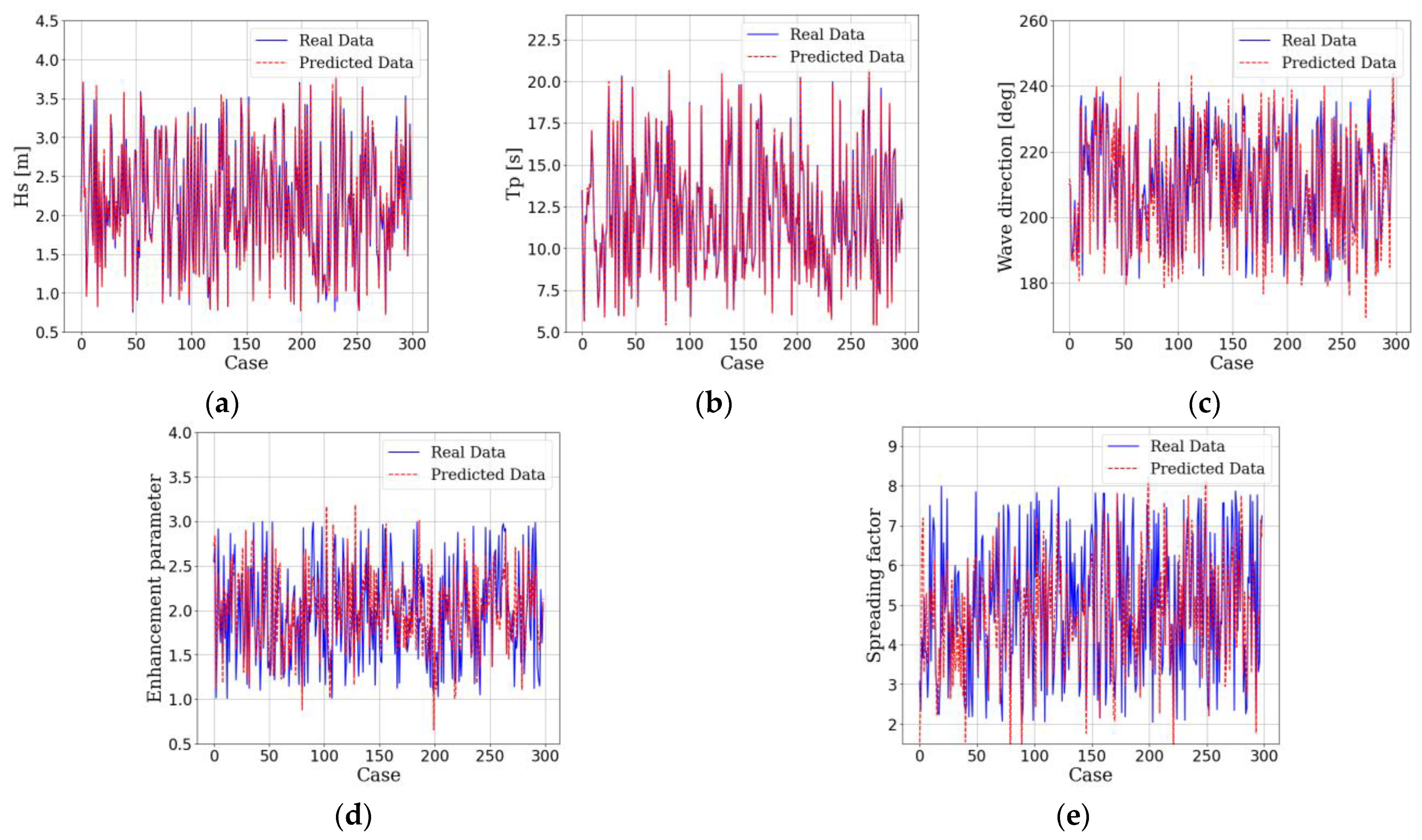
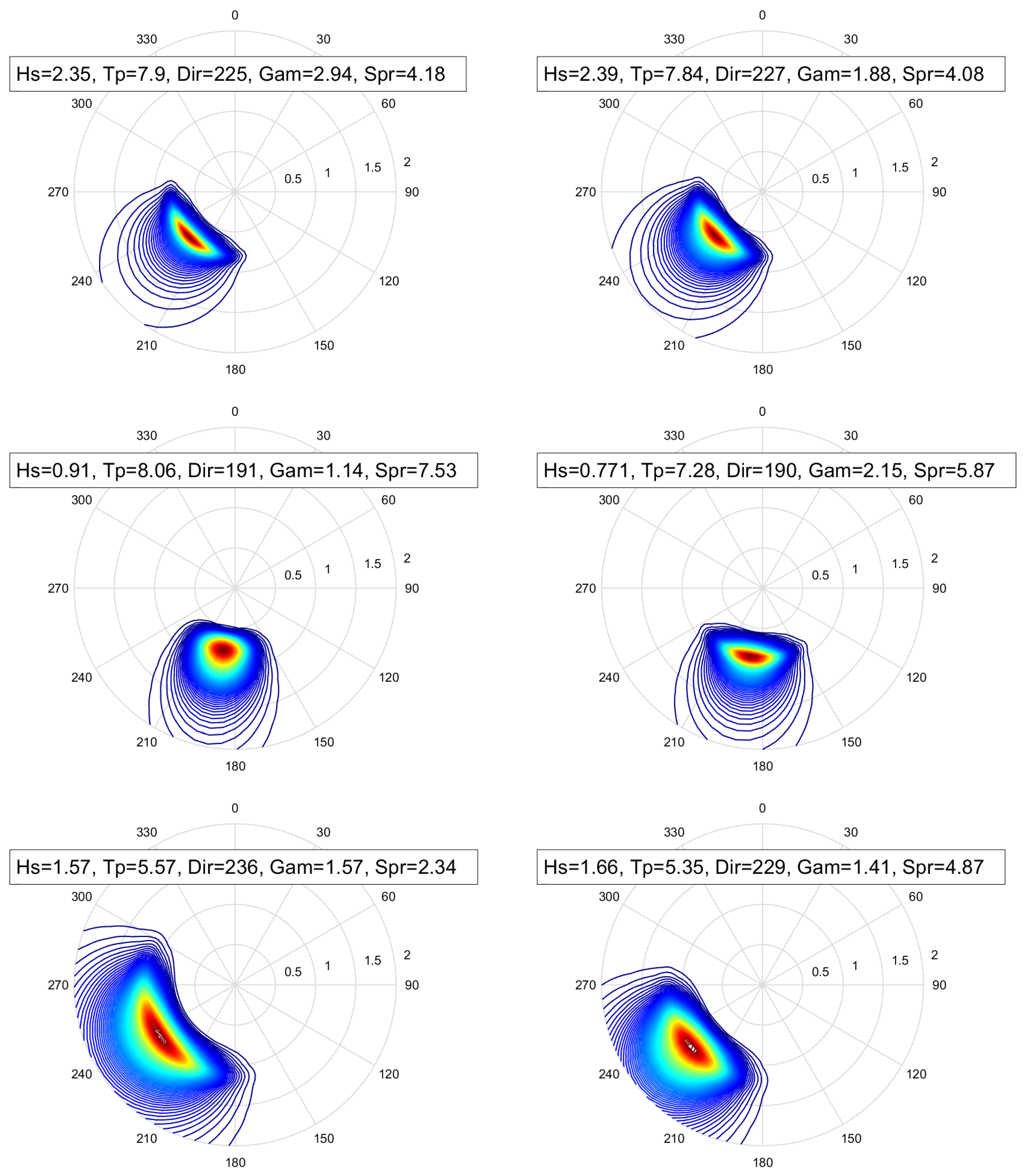
4.3. Estimation of Directional Wave Spectrum

This section presents the best results after various sensitivity tests. As explained earlier, the test datasets are randomly generated in the range of 0.75 m < $H_s$ < 3.75 m, 5.5 s < $T_p$ < 20.5 s, 180° < $\overline{\theta }$ < 240°, 1 < $\gamma$ < 3, and 2 < s < 8. Figure 14 shows the regression plots when all 119 input variables are considered. While these results demonstrate that an extensive set of input parameters can lead to very high R-squared values (0.99 for $H_s$, 1.0 for $T_p$, and 0.9 for $\overline{\theta }$), it is important to recognize that assembling and processing such a large number of statistical inputs may not be practical. Nevertheless, the analysis provides a valuable benchmark, showing the upper performance limit of the model under idealized conditions. This level of accuracy suggests that the ANN model can, in principle, effectively capture the complex relationships between platform motion data and wave parameters. The estimation of wave main direction indicates a strong correlation between predicted and actual values, indicating the model’s ability to discern wave main direction even in directional-spreading conditions. While the $R^2$ values of the enhancement parameter and spreading factor are lower, they still exhibit reasonable prediction, which seems to be improved compared to earlier research [13].

Figure 15 presents direct comparisons of the actual and predicted wave parameters for three hundred test cases. Since an FPSO unit’s downtime is highly related to $H_s$, the exceedingly high accuracy of $H_s$ exhibits robust practical applicability. Again, the enhancement parameter $\gamma$ in the JONSWAP spectrum and the spreading exponent s are randomly selected, making it difficult to identify any correlations with other wave parameters, which explains the relatively low $R^2$ values. In a mild sea environment, the enhancement parameter $\gamma$ and the directional-spreading factor s do not induce strong, distinct effects on vessel motions and thus exhibit weaker correlations with the measured signals. Addressing this issue may involve incorporating more energetic wave cases in training data or devising more specialized feature extraction techniques, which we will pursue in future developments of our modeling approach. Nevertheless, there exist rather consistent trends between the actual and predicted values.

Finally, a comparison of the directional wave spectra of three representative cases is shown in Figure 16. $H_s$, $T_p$, and $\overline{\theta }$ are estimated with high precision, and although the estimated γ and s are less accurately estimated compared to the actual values, the spectra match each other rather well. The slight differences between the left (actual) and right (predicted) results can be attributed to numerical approximations in the ANN model and the inherent limitations of the synthetic dataset. While the synthetic data are designed to emulate realistic environmental conditions, they may not fully capture the complex interactions and dependencies present in actual wave dynamics. Additionally, differences may stem from the limited representation of some parameters in the training data, as indicated by the weaker correlations observed for certain variables, such as the enhancement parameter and spreading factor, in the feature correlation analysis (Figure 8).

So far, all the analysis has been conducted using synthetically generated motion signals, which can be considered an ideal and heuristic case. In the real world, actually measured motion sensor signals are not as accurate and clean as the synthetic data, which may affect the accurate production of some additional statistical parameters, as was performed in this paper. In this case, the use of only basic statistical parameters (like heave–roll–pitch standard deviations) as input may be more practical [38]. Also, there should be some correlation among metocean parameters. For instance, the significant wave height and peak period are highly correlated, such that the higher the wave height, the longer the peak period. Similarly, enhancement parameters and spreading factors are correlated with the significant wave height and peak period. Wave direction is correlated with wind direction for wind seas. So, using actually measured environmental conditions can result in better estimations of the enhancement parameter and spreading factor. This kind of test will be conducted in a future study.

In addition to examining the estimation errors for the five individual parameters ($H_s$, $T_p$, $\overline{\theta }$, $\gamma$, and s), an overall measure of directional-spectrum accuracy can provide useful insights into the cumulative impact of parameter mismatches. One possibility is to use the mean absolute percentage error (MAPE) between the estimated directional spectrum $\widehat{S}\left(\omega ,\theta \right)$ and the reference $S\left(\omega ,\theta \right)$ across all frequencies and directions:

$$MAP{E}_{\omega ,\theta }={\displaystyle \frac{1}{N}}{\displaystyle \sum }_{\forall \left(\omega ,\theta \right)}\left|{\displaystyle \frac{S\left(\omega ,\theta \right)-\widehat{S}\left(\omega ,\theta \right)}{S\left(\omega ,\theta \right)}}\right|\times 100\%$$

(6)

where $N$ is the total number of $\omega$-$\theta$ grid points. Although we only introduce this metric here, a systematic numerical evaluation of these spectrum-level errors for the entire test set will be part of our future work.

5. Conclusions

The present study proposed an ANN model for the inverse estimation of wave parameters using synthetic motion sensor data collected from the digital twin of a moored FPSO unit. After rigorous simulations under varying environmental conditions and a thorough analysis of the motion sensor data, the ANNs were trained and optimized to accurately predict the significant wave height, peak period, main wave direction, enhancement parameter, and directional-spreading factor. The conclusions drawn from the systematic analyses and comparisons of the results are as follows:

• Additional information from accelerations and angular velocities improves the overall prediction accuracy of the significant wave height, peak period, and main wave direction compared to in cases with only 6DOF motions as input.
• Introducing additional multiple motion-based statistical variables to have more correlated inputs significantly enhances the estimation accuracy of all wave parameters.
• Sensitivity tests regarding thresholds show the best performance when using all variables as inputs, with accuracy tending to decrease as the threshold increases, indicating a decrease in accuracy with fewer adopted inputs.
• The optimized ANN algorithms estimate the significant wave height, peak period, and main wave direction with high accuracy, while the enhancement parameter and spreading factor are estimated with reduced accuracy.
• A comparative analysis with other ML methods demonstrates the superiority of ANNs in accurately estimating wave parameters, highlighting their capability to capture complex nonlinear patterns inherent in data.
• Having more relevant statistical parameters as input improves estimation accuracy to some degree with more data processing, but there is a trade-off between accuracy and practicality depending on the data amount and quality needed to collect and process input variables.

In conclusion, the proposed ANN approach presents a robust and practical solution for the inverse estimation of wave parameters from motion sensor data. The high accuracy and efficiency of the models hold significant implications for various maritime applications, including marine navigation, offshore operations, and oceanographic research, contributing to improved safety and efficiency in these maritime activities.

References

1. Bisinotto, G.A.; Cotrim, L.P.; Cozman, F.G.; Tannuri, E.A. Sea state estimation with neural networks based on the motion of a moored fpso subjected to campos basin metocean conditions. In Proceedings of the Brazilian Conference on Intelligent Systems, Online, 29 November–3 December 2021; pp. 294–308. [Google Scholar]
2. Duz, B.; Mak, B.; Hageman, R.; Grasso, N. Real time estimation of local wave characteristics from ship motions using artificial neural networks. In Proceedings of the Practical Design of Ships and Other Floating Structures: Proceedings of the 14th International Symposium, PRADS 2019, Yokohama, Japan, 22–26 September 2019; Volume III, pp. 657–678. [Google Scholar]
3. Mak, B.; Düz, B. Ship As a Wave Buoy: Estimating Relative Wave Direction From In-Service Ship Motion Measurements Using Machine Learning. In Proceedings of the ASME 2019 38th International Conference on Ocean, Offshore and Arctic Engineering, Glasgow, Scotland, UK, 9–14 June 2019. [Google Scholar]
4. Nielsen, U.D.; Mittendorf, M.; Shao, Y.; Storhaug, G. Wave spectrum estimation conditioned on machine learning-based output using the wave buoy analogy. Mar. Struct. 2023, 91, 103470. [Google Scholar] [CrossRef]
5. Scholcz, T.; Düz, B.; Hageman, R.; Mak, B. Consistency assessment of wave directional spectrum predictions from machine learning based ship-as-a-wave-buoy methods. In Proceedings of the International Conference on Offshore Mechanics and Arctic Engineering, Boston, MA, USA, 7–8 December 2022; p. V05BT06A004. [Google Scholar]
6. Scholcz, T.; Mak, B. Ship as a wave buoy: Estimating full directional wave spectra from in-service ship motion measurements using deep learning. In Proceedings of the International Conference on Offshore Mechanics and Arctic Engineering, Virtual, 3–7 August 2020; p. V001T001A006. [Google Scholar]
7. Chen, X.; Okada, T.; Kawamura, Y.; Mitsuyuki, T. Estimation of on-site directional wave spectra using measured hull stresses on 14,000 TEU large container ships. J. Mar. Sci. Technol. 2020, 25, 690–706. [Google Scholar] [CrossRef]
8. Han, P.; Li, G.; Cheng, X.; Skjong, S.; Zhang, H. An uncertainty-aware hybrid approach for sea state estimation using ship motion responses. IEEE Trans. Ind. Inform. 2021, 18, 891–900. [Google Scholar] [CrossRef]
9. Han, P.; Li, G.; Skjong, S.; Wu, B.; Zhang, H. Data-driven sea state estimation for vessels using multi-domain features from motion responses. In Proceedings of the 2021 IEEE International Conference on Robotics and Automation (ICRA), Xi’an, China, 30 May–5 June 2021; pp. 2120–2126. [Google Scholar]
10. Mittendorf, M.; Nielsen, U.D.; Bingham, H.B. The prediction of sea state parameters by deep learning techniques using ship motion data. In Proceedings of the 7th World Maritime Technology Conference (WMTC’22), Copenhagen, Denmark, 26–28 April 2022. [Google Scholar]
11. Nielsen, U.D.; Bingham, H.B.; Brodtkorb, A.H.; Iseki, T.; Jensen, J.J.; Mittendorf, M.; Mounet, R.E.; Shao, Y.; Storhaug, G.; Sørensen, A.J. Estimating waves via measured ship responses. Sci. Rep. 2023, 13, 17342. [Google Scholar] [CrossRef]
12. Cheng, X.; Li, G.; Ellefsen, A.L.; Chen, S.; Hildre, H.P.; Zhang, H. A novel densely connected convolutional neural network for sea-state estimation using ship motion data. IEEE Trans. Instrum. Meas. 2020, 69, 5984–5993. [Google Scholar] [CrossRef]
13. Han, P.; Li, G.; Skjong, S.; Zhang, H. Directional wave spectrum estimation with ship motion responses using adversarial networks. Mar. Struct. 2022, 83, 103159. [Google Scholar] [CrossRef]
14. Kawai, T.; Kawamura, Y.; Okada, T.; Mitsuyuki, T.; Chen, X. Sea state estimation using monitoring data by convolutional neural network (CNN). J. Mar. Sci. Technol. 2021, 26, 947–962. [Google Scholar] [CrossRef]
15. Mittendorf, M.; Nielsen, U.D.; Bingham, H.B.; Storhaug, G. Sea state identification using machine learning—A comparative study based on in-service data from a container vessel. Mar. Struct. 2022, 85, 103274. [Google Scholar] [CrossRef]
16. Mounet, R.E.; Chen, J.; Nielsen, U.D.; Brodtkorb, A.H.; Pillai, A.C.; Ashton, I.G.; Steele, E.C. Deriving spatial wave data from a network of buoys and ships. Ocean. Eng. 2023, 281, 114892. [Google Scholar] [CrossRef]
17. Nielsen, U.D.; Dietz, J. Estimation of sea state parameters by the wave buoy analogy with comparisons to third generation spectral wave models. Ocean. Eng. 2020, 216, 107781. [Google Scholar] [CrossRef]
18. Kim, S.; Kim, M.-H. Dynamic behaviors of conventional SCR and lazy-wave SCR for FPSOs in deepwater. Ocean. Eng. 2015, 106, 396–414. [Google Scholar] [CrossRef]
19. Kim, S.; Kim, M.; Kang, H. Turret location impact on global performance of a thruster-assisted turret-moored FPSO. Ocean Syst. Eng. Int. J 2016, 6, 265–287. [Google Scholar] [CrossRef]
20. Orcina, L. OrcaFlex User Manual; Version 11.0 B; Orcina: Ulverston, UK, 2016. [Google Scholar]
21. Lee, C.-H. WAMIT Theory Manual; Massachusetts Institute of Technology, Department of Ocean Engineering: Cambridge, MA, USA, 1995. [Google Scholar]
22. Hersbach, H.; Bell, B.; Berrisford, P.; Hirahara, S.; Horányi, A.; Muñoz-Sabater, J.; Nicolas, J.; Peubey, C.; Radu, R.; Schepers, D. The ERA5 global reanalysis. Q. J. R. Meteorol. Soc. 2020, 146, 1999–2049. [Google Scholar] [CrossRef]
23. Chassignet, E.P.; Hurlburt, H.E.; Smedstad, O.M.; Halliwell, G.R.; Hogan, P.J.; Wallcraft, A.J.; Baraille, R.; Bleck, R. The HYCOM (hybrid coordinate ocean model) data assimilative system. J. Mar. Syst. 2007, 65, 60–83. [Google Scholar] [CrossRef]
24. Huang, Y.; He, Y.; Liu, Y.; Qiu, M.; Li, M.; Luo, Z.; Xu, J. Study of the response characteristics of a spread moored FPSO in the bidirectional sea state. Ocean. Eng. 2022, 264, 112453. [Google Scholar] [CrossRef]
25. Lopez, J.T.; Tao, L.; Xiao, L.; Hu, Z. Experimental study on the hydrodynamic behaviour of an FPSO in a deepwater region of the Gulf of Mexico. Ocean. Eng. 2017, 129, 549–566. [Google Scholar] [CrossRef]
26. Kim, H.; Kang, H.; Kim, M.-H. Real-time inverse estimation of ocean wave spectra from vessel-motion sensors using adaptive kalman filter. Appl. Sci. 2019, 9, 2797. [Google Scholar] [CrossRef]
27. Kim, H.; Park, J.; Jin, C.; Kim, M.; Lee, D. Real-time inverse estimation of multi-directional random waves from vessel-motion sensors using Kalman filter. Ocean. Eng. 2023, 280, 114501. [Google Scholar] [CrossRef]
28. Keras Documentation. 2015. Available online: https://keras.io/ (accessed on 2 December 2024).
29. Abadi, M.; Barham, P.; Chen, J.; Chen, Z.; Davis, A.; Dean, J.; Devin, M.; Ghemawat, S.; Irving, G.; Isard, M. {TensorFlow}: A system for {Large-Scale} machine learning. In Proceedings of the 12th USENIX Symposium on Operating Systems Design and Implementation (OSDI 16), Savannah, GA, USA, 2–4 November 2016; pp. 265–283. [Google Scholar]
30. George, A.; Poguluri, S.K.; Kim, J.; Cho, I.H. Design optimization of a multi-layer porous wave absorber using an artificial neural network model. Ocean. Eng. 2022, 265, 112666. [Google Scholar] [CrossRef]
31. Velasco-Gallego, C.; Lazakis, I. Real-time data-driven missing data imputation for short-term sensor data of marine systems. A comparative study. Ocean. Eng. 2020, 218, 108261. [Google Scholar] [CrossRef]
32. Xie, J.; Xue, X. A novel hybrid model based on grey wolf optimizer and group method of data handling for the prediction of monthly mean significant wave heights. Ocean. Eng. 2023, 284, 115274. [Google Scholar] [CrossRef]
33. Juan, N.P.; Matutano, C.; Valdecantos, V.N. Uncertainties in the application of artificial neural networks in ocean engineering. Ocean. Eng. 2023, 284, 115193. [Google Scholar] [CrossRef]
34. Zhang, J.; Lu, W.; Li, J.; Li, X.; Cheng, Z. A data-driven methodology for wave time-series measurement on floating structures. Ocean. Eng. 2024, 303, 117629. [Google Scholar] [CrossRef]
35. Han, X.; Zhang, Z.; Ding, N.; Gu, Y.; Liu, X.; Huo, Y.; Qiu, J.; Yao, Y.; Zhang, A.; Zhang, L. Pre-trained models: Past, present and future. AI Open 2021, 2, 225–250. [Google Scholar] [CrossRef]
36. Panda, J. Machine learning for naval architecture, ocean and marine engineering. J. Mar. Sci. Technol. 2023, 28, 1–26. [Google Scholar] [CrossRef]
37. Schmidgall, S.; Ziaei, R.; Achterberg, J.; Kirsch, L.; Hajiseyedrazi, S.; Eshraghian, J. Brain-inspired learning in artificial neural networks: A review. APL Mach. Learn. 2024, 2, 021501. [Google Scholar] [CrossRef]
38. Kwon, D.-S.; Jin, C.; Kim, M.; Guha, A.; Esenkov, O.E.; Ryu, S. Inverse wave estimation from measured FPSO motions through artificial neural networks. In Proceedings of the SNAME Offshore Symposium, Houston, TX, USA, 20 February 2024; p. D011S004R003. [Google Scholar]
Figure 1. Designed FPSO model with mooring lines (orange lines) and steel catenary riser (blue line).
Jmse 13 00069 g001
Figure 2. Wave scatter diagram, where numbers in the diagram are occurrence (a), wave rose (b), wind rose (c), and current rose values (d) (longitude: −56 degrees E; latitude: 10 degrees N; it is from this direction that waves, winds, and currents are coming, and all directions are measured clockwise from the north).
Jmse 13 00069 g002
Figure 3. Training (red box) and test (blue box) datasets for environmental conditions ((a): wind speed; (b): wind direction; (c): current speed; (d): current direction; (e): significant wave height; (f): peak period; (g): wave direction; (h): enhancement parameter; (i): spreading factor).
Jmse 13 00069 g003
Figure 4. Wave conditions for the training set for ML based on ERA5 data.
Jmse 13 00069 g004
Figure 5. Time series and spectra of wave elevation and 6DOF motion displacements.
Jmse 13 00069 g005
Figure 6. Layout of feedforward algorithm.
Jmse 13 00069 g006
Figure 7. Architecture of ANN for estimating directional wave spectrum.
Jmse 13 00069 g007
Figure 8. Feature correlation heatmap of input variables and wave parameters (in the figure, mean and std stand for mean value and standard deviation; STDR stands for relative standard deviation; m0, m2, and m4 represent the zeroth, second, and fourth spectral moments; T c , T z , and BW are the mean crest periods, the mean up-crossing periods, and the spectral bandwidth; the numbers 1–6 represent surge, sway, heave, roll, pitch, and yaw displacements, 7–9 denote angular velocities with respect to the x, y, and z axes, and 10–12 represent x, y, and z accelerations, respectively).
Jmse 13 00069 g008
Figure 9. Series plot of 1200 cases— H s and a large correlation (m4_10: the fourth spectral moments of surge acceleration), median correlation (m4_11: the fourth spectral moments of sway acceleration), and low correlation ( T c _11: crest period of sway acceleration) with H s , respectively.
Jmse 13 00069 g009
Figure 10. Regression plots for the estimation of each wave parameter using the mean and standard deviation of 6DOF motions as input (the number of inputs = 12) ((a): significant wave height; (b): wave peak period; (c): wave direction; (d): enhancement parameter; (e): spreading factor).
Jmse 13 00069 g010
Figure 11. Regression plots for the estimation of each wave parameter using the mean and standard deviation of 12DOF motions as input (the number of inputs = 24) ((a): significant wave height; (b): wave peak period; (c): wave direction; (d): enhancement parameter; (e): spreading factor).
Jmse 13 00069 g011
Figure 12. Regression plots for the estimation of main wave direction while applying thresholds to correlations between input and output variables ((a): 119 input variables; (b): more than 10% correlated variables; (c): more than 20% correlated variables; (d): more than 30% correlated variables; (e): more than 40% correlated variables; (f): more than 50% correlated variables).
Jmse 13 00069 g012
Figure 13. R 2 values of wave parameters from different ML models.
Jmse 13 00069 g013
Figure 14. Regression plots for the estimation of each wave parameter using 119 input variables ((a): significant wave height; (b): wave peak period; (c): wave direction; (d): enhancement parameter; (e): spreading factor).
Jmse 13 00069 g014
Figure 15. Series plot for the estimation of each wave parameter using 119 input variables ((a): significant wave height; (b): wave peak period; (c): wave direction; (d): enhancement parameter; (e): spreading factor).
Jmse 13 00069 g015
Figure 16. Comparison of directional wave spectra (left = actual; right = estimated).
Jmse 13 00069 g016