


The Optimization of Four Key Parameters in the XBeach Model by GLUE Method: Taking Chudao South Beach as an Example


Abstract
:1. Introduction
2. Data and Methods
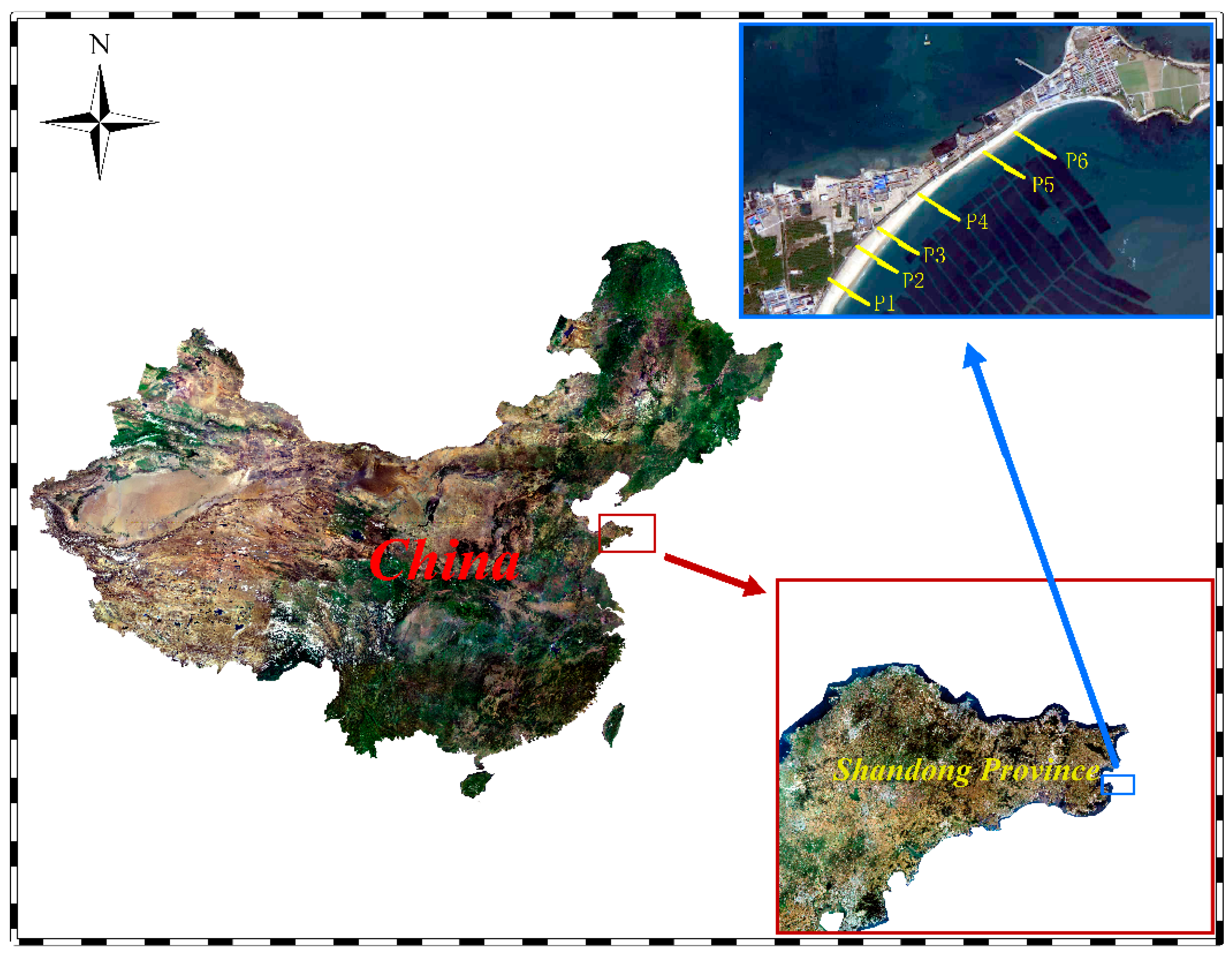
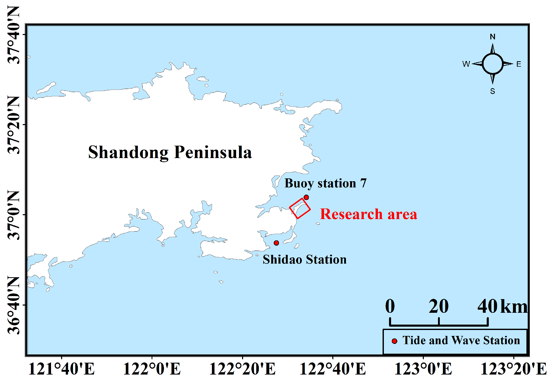
2.1. Study Area
2.2. Introduction of XBeach
2.3. Model Setting
2.3.1. Terrain Condition
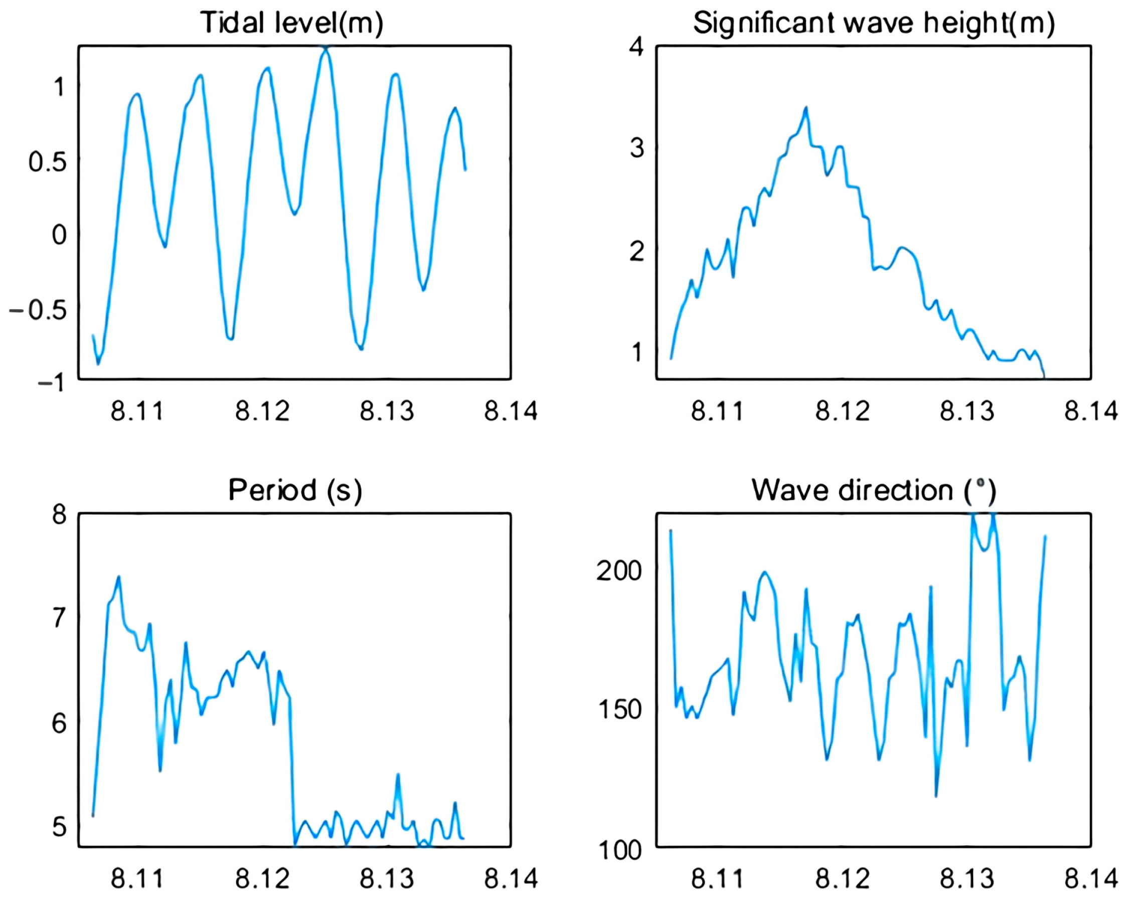
2.3.2. Tide Level and Wave Boundary
3. GLUE Method
3.1. Parameter Sets Generation and Evaluation
3.2. Parameter Optimization Method
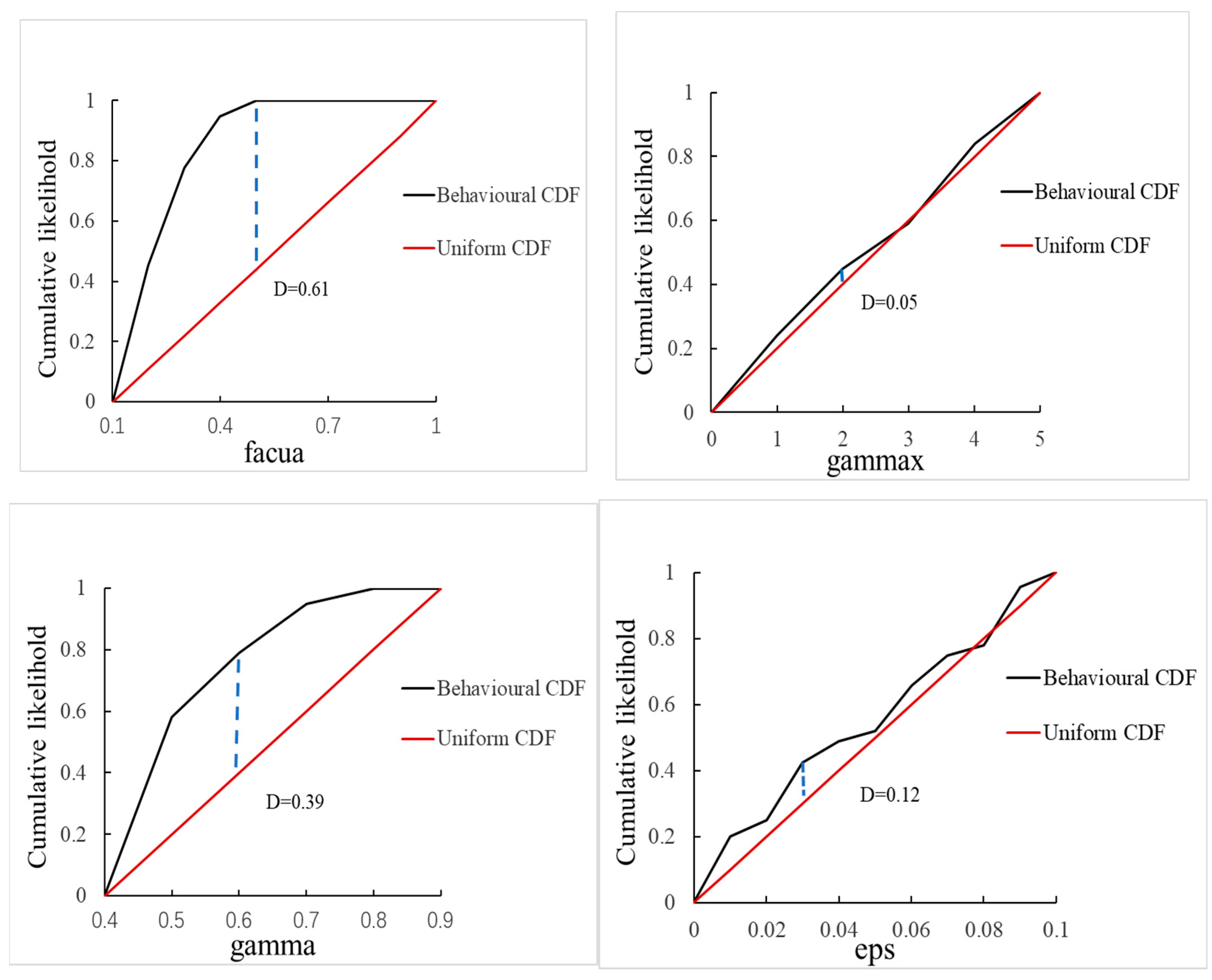
3.2.1. Parameter Sensitivity Processing
3.2.2. Parameter Optimization Selection
3.3. GLUE Establishment
4. Results
4.1. Sensitivity Analysis
4.2. Parameter Optimization Analysis
5. Discussions
6. Conclusions
Author Contributions
Funding
Institutional Review Board Statement
Informed Consent Statement
Data Availability Statement
Conflicts of Interest
References
- Jackson, N.L.; Nordstrom, K.F.; Farrell, E.J. Longshore sediment transport and foreshore change in the swash zone of an estuarine beach. Mar. Geol. 2017, 386, 88–97. [Google Scholar] [CrossRef]
- Boccotti, P. Wave Mechanics for Ocean Engineering; Elsevier: Amsterdam, The Netherlands, 2000. [Google Scholar]
- de Vries, J.V.T.; Van Gent, M.; Walstra, D.; Reniers, A. Analysis of dune erosion processes in large-scale flume experiments. Coast. Eng. 2008, 55, 1028–1040. [Google Scholar] [CrossRef]
- Daly, C. Low Frequency Waves in the Shoaling and Nearshore Zone a Validation of XBeach. Master’s Thesis, Technical University of Delft, Delft, The Netherlands, 2009. [Google Scholar]
- Roelvink, D.; Reniers, A.; Van Dongeren, A.; De Vries, J.V.T.; McCall, R.; Lescinski, J. Modelling storm impacts on beaches, dunes and barrier islands. Coast. Eng. 2009, 56, 1133–1152. [Google Scholar] [CrossRef]
- Kombiadou, K.; Costas, S.; Roelvink, D. Simulating Destructive and Constructive Morphodynamic Processes in Steep Beaches. J. Mar. Sci. Eng. 2021, 9, 86. [Google Scholar] [CrossRef]
- McCall, R.T.; de Vries, J.; Plant, N.G.; Van Dongeren, A.R.; Roelvink, J.A.; Thompson, D.M.; Reniers, A. Two-dimensional time dependent hurricane overwash and erosion modeling at Santa Rosa Island. Coast. Eng. 2010, 57, 668–683. [Google Scholar] [CrossRef]
- Kuang, C.P.; Fan, J.D.; Han, X.J.; Li, H.Y.; Qin, R.F.; Zou, Q.P. Numerical Modelling of Beach Profile Evolution with and without an Artificial Reef. Water 2023, 15, 3832. [Google Scholar] [CrossRef]
- Yu, H.; Weng, Z.H.; Chen, G.F.; Chen, X. Improved XBeach model and its application in coastal beach evolution under wave action. Coast. Eng. J. 2023, 65, 560–571. [Google Scholar] [CrossRef]
- Pender, D.; Karunarathna, H. A statistical-process based approach for modelling beach profile variability. Coast. Eng. 2013, 81, 19–29. [Google Scholar] [CrossRef]
- Callaghan, D.; Nielsen, P.; Short, A.; Ranasinghe, R. Statistical simulation of wave climate and extreme beach erosion. Coast. Eng. 2008, 55, 375–390. [Google Scholar] [CrossRef]
- Liu, X.; Kuang, C.; Huang, S.; Dong, W. Modelling morphodynamic responses of a natural embayed beach to Typhoon Lekima encountering different tide types. Anthr. Coasts 2022, 5, 4. [Google Scholar] [CrossRef]
- Mickey, R.C.; Dalyander, P.S.; McCall, R.; Passeri, D.L. Sensitivity of Storm Response to Antecedent Topography in the XBeach Model. J. Mar. Sci. Eng. 2020, 8, 829. [Google Scholar] [CrossRef]
- Splinter, K.D.; Palmsten, M.L. Modeling dune response to an East Coast Low. Mar. Geol. 2012, 329, 46–57. [Google Scholar] [CrossRef]
- Stockdon, H.F.; Thompson, D.M.; Plant, N.G.; Long, J.W. Evaluation of wave runup predictions from numerical and parametric models. Coast. Eng. 2014, 92, 4. [Google Scholar] [CrossRef]
- Harley, M.; Armaroli, C.; Ciavola, P. Evaluation of XBeach predictions for a real-time warning system in Emilia-Romagna, Northern Italy. J. Coast. Res. 2011, 64, 1861–1865. [Google Scholar]
- Beven, K.; Binley, A. The future of distributed models: Model calibration and uncertainty prediction. Hydrol. Process. 1992, 6, 279–298. [Google Scholar] [CrossRef]
- Xing, H.; Li, P.P.; Zhang, L.L.; Xue, H.Y.; Shi, H.Y.; You, Z.J. Numerical Simulation of the Beach Response Mechanism under Typhoon Lekima: A Case Study of the Southern Beach of Chudao. J. Mar. Sci. Eng. 2023, 11, 1156. [Google Scholar] [CrossRef]
- Simmons, J.A.; Harley, M.D.; Marshall, L.A.; Turner, I.L.; Splinter, K.D.; Cox, R.J. Calibrating and assessing uncertainty in coastal numerical models. Coast. Eng. 2017, 125, 28–41. [Google Scholar] [CrossRef]
- Zhang, Q.X. Tri-dimensional breeding in Sanggou Bay. Mar. Sci. 1988, 12, 57. [Google Scholar]
- Zheng, H.P.; Zhang, Y.; Wang, Y.; Zhang, L.F.; Peng, J.; Liu, S.S.; Li, A.B. Characteristics of Atmospheric Kinetic Energy Spectra during the Intensification of Typhoon Lekima (2019). Appl. Sci. 2020, 10, 6029. [Google Scholar] [CrossRef]
- Batchelor, G.K. An Introduction to Fluid Dynamics; Cambridge University Press: Cambridge, UK, 2000. [Google Scholar]
- Holthuijsen, L.; Booij, N.; Herbers, T. A prediction model for stationary, short-crested waves in shallow water with ambient currents. Coast. Eng. 1989, 13, 23–54. [Google Scholar] [CrossRef]
- Phillips, O. The Dynamics of the Upper Ocean, 2nd ed.; Cambridge University Press: Cambridge, UK, 1982. [Google Scholar]
- Galappatti, G.; Vreugdenhil, C. A depth-integrated model for suspended sediment transport. J. Hydraul. Res. 1985, 23, 359–377. [Google Scholar] [CrossRef]
- Harley, M.D.; Valentini, A.; Armaroli, C.; Perini, L.; Calabrese, L.; Ciavola, P. Can an early-warning system help minimize the impacts of coastal storms? A case study of the 2012 Halloween storm, northern Italy. Nat. Hazards Earth Syst. Sci. 2016, 16, 209–222. [Google Scholar] [CrossRef]
- Zhang, X.R.; Shi, H.Y.; Liu, Z.Y.; Li, H.Q.; Xing, H.; Wang, L.Y. The response of Chudao’s beach to typhoon “Lekima” (No. 1909). Open Geosci. 2022, 14, 813–823. [Google Scholar] [CrossRef]
- Lahiri, K.; Yang, L. Asymptotic variance of Brier (skill) score in the presence of serial correlation. Econ. Lett. 2016, 141, 125–129. [Google Scholar] [CrossRef]
- van Rijn, L.C.; Walstra, D.J.; Grasmeijer, B.; Sutherland, J.; Pan, S.; Sierra, J. The predictability of cross-shore bed evolution of sandy beaches at the time scale of storms and seasons using process-based profile models. Coast. Eng. 2003, 47, 295–327. [Google Scholar] [CrossRef]
- He, J.Q.; Jones, J.W.; Graham, W.D.; Dukes, M.D. Influence of likelihood function choice for estimating crop model parameters using the generalized likelihood uncertainty estimation method. Agric. Syst. 2010, 103, 256–264. [Google Scholar] [CrossRef]
- Beven, K. A manifesto for the equifinality thesis. J. Hydrol. 2006, 320, 18–36. [Google Scholar] [CrossRef]
- Spear, R.C.; Hornberger, G.M. Eutrophication in peel inlet—II. Identification of critical uncertainties via generalized sensitivity analysis. Water Res. 1980, 14, 43–49. [Google Scholar] [CrossRef]
- Jakeman, A.; Ghassemi, F.; Dietrich, C.; Musgrove, T.; Whitehead, P. Calibration and reliability of an aquifer system model using generalized sensitivity analysis. In Proceedings of the Conference, Hague, The Netherlands, 3–6 September 1990; No. 195. Available online: https://www.scirp.org/reference/referencespapers?referenceid=2346939 (accessed on 9 March 2025).
- Thorndahl, S.; Beven, K.J.; Jensen, J.B.; Schaarup-Jensen, K. Event based uncertainty assessment in urban drainage modelling, applying the GLUE methodology. J. Hydrol. 2008, 357, 421–437. [Google Scholar] [CrossRef]
- Roelvink, J.; Reniers, A.; Dongeren, A.; Dongeren, A.; Van, T.; Mccall, R. XBeach Model—Description and Manual. 2010. Available online: https://www.researchgate.net/publication/257305748_XBeach_Model_-_Description_and_Manual (accessed on 9 March 2025).
- Ragab, R.; Kaelin, A.; Afzal, M.; Panagea, I. Application of Generalized Likelihood Uncertainty Estimation (GLUE) at different temporal scales to reduce the uncertainty level in modelled river flows. Hydrol. Sci. J. 2020, 65, 1856–1871. [Google Scholar] [CrossRef]


| Parameters | Meanings | Default Values | Recommended Ranges |
|---|---|---|---|
| facua | The degree to which wave tilt and asymmetry affect sediment transport direction | 0.1 | 0–1 |
| gamma | The breaking parameter in wave dissipation models | 0.55 | 0.4–0.9 |
| gammax | The maximum allowable ratio between wave height and water depth | 2 | 0.4–5 |
| eps | Threshold water depth above which cells are considered wet (m) | 0.005 | 0.001–0.1 |
| The Range of BSS Values | The Predictive Effect |
|---|---|
| 1~0.8 | Excellent |
| 0.8~0.5 | Good |
| 0.5~0.3 | Reasonable |
| 0.3~0 | Poor |
| <0 | Bad |
| Profiles | BSS Before Parameter Calibration | BSS After Parameter Calibration |
|---|---|---|
| P1 | 0.30 | 0.68 |
| P6 | 0.17 | 0.79 |
| Profile | Measured Unit Erosion–Deposition Volume/m3 | Imulated Unit Erosion–Deposition Volume with Default Parameters/m3 | Simulated Unit Erosion–Deposition Volume After Parameter Tuning/m3 |
|---|---|---|---|
| P1 | −7.2 | −17.4 | −8.5 |
| P6 | −5.3 | −17.2 | −8.8 |
| Profiles | P2 | P3 | P4 | P5 |
|---|---|---|---|---|
| Calculated BSS values using default parameters | 0.64 | −0.22 | 0.82 | 0.22 |
| Calculated BSS values using optimized parameters | 0.80 | 0.33 | 0.76 | 0.81 |
| Profile | Measured Unit Erosion–Deposition Volume/m3 | Simulated Unit Erosion–Deposition Volume With Default Parameters/m3 | Simulated Unit Erosion–Deposition Volume After Parameter Tuning/m3 |
|---|---|---|---|
| P2 | −8.5 | −18.1 | −11.5 |
| P3 | −10.0 | −25.1 | −17.0 |
| P4 | −15.0 | −24.1 | −12.5 |
| P5 | −16.4 | −32.7 | −19.7 |
Disclaimer/Publisher’s Note: The statements, opinions and data contained in all publications are solely those of the individual author(s) and contributor(s) and not of MDPI and/or the editor(s). MDPI and/or the editor(s) disclaim responsibility for any injury to people or property resulting from any ideas, methods, instructions or products referred to in the content. |
© 2025 by the authors. Licensee MDPI, Basel, Switzerland. This article is an open access article distributed under the terms and conditions of the Creative Commons Attribution (CC BY) license (https://creativecommons.org/licenses/by/4.0/).
Share and Cite
Gai, Y.; Li, L.; Li, Z.; Shi, H. The Optimization of Four Key Parameters in the XBeach Model by GLUE Method: Taking Chudao South Beach as an Example. J. Mar. Sci. Eng. 2025, 13, 555. https://doi.org/10.3390/jmse13030555
Gai Y, Li L, Li Z, Shi H. The Optimization of Four Key Parameters in the XBeach Model by GLUE Method: Taking Chudao South Beach as an Example. Journal of Marine Science and Engineering. 2025; 13(3):555. https://doi.org/10.3390/jmse13030555
Chicago/Turabian StyleGai, Yunyun, Longsheng Li, Zikang Li, and Hongyuan Shi. 2025. "The Optimization of Four Key Parameters in the XBeach Model by GLUE Method: Taking Chudao South Beach as an Example" Journal of Marine Science and Engineering 13, no. 3: 555. https://doi.org/10.3390/jmse13030555
APA StyleGai, Y., Li, L., Li, Z., & Shi, H. (2025). The Optimization of Four Key Parameters in the XBeach Model by GLUE Method: Taking Chudao South Beach as an Example. Journal of Marine Science and Engineering, 13(3), 555. https://doi.org/10.3390/jmse13030555