Abstract
Modeling and system identification are critical for the design, simulation, and navigation of underwater vehicles. This study presents a six degree-of-freedom (DoF) nonlinear model for a finless underactuated underwater vehicle, incorporating port-starboard symmetry and cross-flow terms. Then, hydrodynamic damping parameters are identified using an optimized Extended Kalman Filter (EKF), establishing a steady validation framework for computational fluid dynamics (CFD) simulation coefficients. Additionally, system identification is further enhanced with a Long Short-Term Memory (LSTM) neural network and a comprehensive dataset construction method, enabling time-series predictions of linear and angular velocities. To mitigate position divergence in dead reckoning (DR) caused by LSTM, a Nonlinear Explicit Complementary Filter (NECF) is integrated for attitude estimation, providing accurate yaw computation and reliable localization without dependence on acoustic sensors or machine vision. Finally, validation and evaluation are conducted to demonstrate model accuracy, EKF convergence, and the reliability of LSTM-based navigation.
1. Introduction
Underwater vehicles are classified based on their control methods into remotely operated underwater vehicles (ROVs), and autonomous underwater vehicles (AUVs). These vehicles are influenced by hydrodynamic forces and moments, as well as environmental disturbances such as waves and currents, leading to strong coupling, nonlinearity, and significant uncertainty [1]. Consequently, the modeling and identification of underwater vehicles have been significant research topics for an extended period.
The mathematical models for underwater vehicles are similar to those for ships, divided into integrated and separated structure models. The integrated model, introduced by Abkowitz [2] in the 1960s, treats the entire vehicle as a single unit. Chislett [3] further developed this using a planar motion mechanism (PMM) for mariner ship simulations. In the 1970s, the Japanese Towing Tank Committee developed the separated (MMG) model [4], which considers the hull, propeller, and rudder independently, allowing for detailed interaction calculations. Modern underwater vehicle modeling builds on these foundational approaches. As detailed in [1], hydrodynamic damping encompasses dissipative forces arising from forced oscillation, surface friction, lift, and vortices. In [5], Gertler and Hagen provided simplified equations for the standard motion dynamics of over 25 submarines, reflecting practical physical behaviors. Once theoretical models are established, the focus often shifts to applying these dynamic models to underwater vehicles [6,7]. Studies on ocean currents [8] underscore the importance of model accuracy for navigation assistance. However, accurately determining parameters for complex underwater dynamic models poses significant challenges, compounded by uncertainties from payload variations. To tackle this, [9] proposed a machine learning-based exploration method, but its reliability remains unverified. Underwater vehicle models are essential for control, simulation, and autonomous navigation, broadly categorized as linear or nonlinear. Linear models offer basic approximations suitable for simpler control strategies, while nonlinear models, often in state-space form, provide more accuracy, albeit with complex computations. Regardless of the model type, the key challenge lies in selecting the most suitable model and reliably identifying parameters to enhance physical fidelity, typically achieved through system identification.
Underwater vehicle physical models contain numerous unknown hydrodynamic parameters [10,11]. Traditional model-based control methods rely on these models, necessitating system identification or parameter identification to determine the unknown hydrodynamic terms. This often involves conducting experiments in towing tanks or PMM with full-scale robots or scaled-down models [12,13]. However, such experiments are time-consuming, requires specialized test platforms, and can be impractical for researchers lacking experimental facilities. Additionally, measurement errors in collected data can be substantial, sometimes reaching 50% [14]. To tackle these challenges, sensor-based identification methods have emerged as simpler, more convenient, and cost-effective alternatives. Goheen and Jefferys pioneered sensor-based system identification for underwater vehicles [15]. Subsequent research proposed an Extended Kalman Filter (EKF) method for identifying surge direction in AUVs using a simplified model [16]. Other studies validated least squares (LS) identification for nonlinear models on specific underwater vehicle [17]. Combining LS and EKF for system identification showed improved results in [18]. Further developments included LS identification for the ROMEO ROV’s four-degree-of-freedom model [19] and improved ROV modeling by considering thruster–body interactions [20]. Smallwood and Whitcomb introduced online adaptive identification, showing its superiority over LS but limited to single-degree-of-freedom dynamics [21]. As traditional methods became standard, the focus shifted to modern approaches. Neural network-based auxiliary system identification methods were introduced to enhance accuracy [22]. The use of total least squares (TLS) for multi-degree-of-freedom models provided robust identification results [23]. An improved multi-output Gaussian orocess (MOGP) was used to effectively model the dynamics of an underactuated AUV, enabling the system to provide confidence measurements [24]. Validation of the modified dual unscented Kalman filter (MDUKF) demonstrated its feasibility for online parameter estimation [25]. Least square support vector machines (LS-SVM) were introduced for effective hydrodynamic parameter estimation [26]. An adaptive identification method was proposed for fully actuated ROVs, requiring only thrust, position, and velocity data [27]. Comprehensive measurement of hydrodynamic parameters using EKF offered more detailed results compared to simplified measurements [28]. A few-shot identification method that combines RMAS with neural networks, significantly improving the accuracy of stochastic dynamical system identification using minimal samples, can be adapted for underwater vehicle modeling [29].
As identification methods have proliferated, selecting the optimal algorithm for efficiency and accuracy is crucial. Research indicates that the unscented Kalman filter (UKF) and transformed UKF outperform EKF, especially when dealing with nonlinear viscous drag [30,31]. Radial basis function (RBF) neural networks have been used for ROV model identification [32], while a PSO-based SVM algorithm was proposed to address multicollinearity in hydrodynamic term identification within the Abkowitz model [33]. The symbolic regression (SR) algorithm has been shown to offer higher fitting accuracy for underwater robot system identification [34]. The extended Kalman particle filter (EKPF) demonstrated a smaller standard deviation in offline identification compared to traditional methods [35], and an optimized UKF showed slight improvements over standard UKF, though with minimal impact on control precision [36]. In the domain of online identification for AUVs, various deep learning methods have been assessed, including neural networks (NN), support vector regression (SVR), Gaussian process regression (GPR), and kernel ridge regression (KRR), with their performance evaluated across different data volumes and computational complexities [37]. Enhanced algorithms like weight distance squared exponential SVR (WDSE-SVR) have shown superior performance in identifying 3 degree-of-freedom (DoF) coupled dynamics models compared to standard TLS and SVR [38]. Dynamic state changes were accurately predicted by altering the AUV’s dynamics and employing incremental SVR (IncSVR) and a data update method, focusing on the decoupled drag term [39,40]. A combined approach using WDSE, IncSVR, and data update strategies led to the development of a method based on Long Short-Term Memory (LSTM) for online identification of nonlinear, coupled and dynamically changing AUV models, achieving precision close to offline identification [41]. Additionally, nonlinear model identification and validation were achieved using orthogonal forward regression (OFR) with ultra-short baseline (USBL) and a Doppler log [42], while a universal adaptive stabilizer (UAS)-based algorithm was developed for parameter identification without relying on position information [43]. A universal adaptive stabilizer (UAS)-based algorithm was also developed for parameter identification without the need for position information [43]. Gaussian process learning (GPL) was employed in [44] to develop nonparametric vehicle dynamics.
To expand the application of system identification and highlight the advantages of non-parametric models, this study integrates system identification with state estimation and onboard sensors to achieve accurate underwater navigation through dead reckoning (DR). To mitigate error accumulation from velocity predictions, a Nonlinear Explicit Complementary Filter (NECF) is adopted [45]. NECF combines gyroscopic measurements with accelerometer and magnetometer data for angle correction, introducing two key improvements: (1) filtering magnetic field components susceptible to interference; and (2) dynamically adjusting weighting coefficients based on sensor confidence, enhancing flexibility. This approach is effective for near-horizontal motion. Its application in simultaneous localization and mapping enables 3D reconstruction [46]. Furthermore, [47] compares 15 positioning algorithms, demonstrating that NECF-based methods achieve minimal error across diverse motion patterns, making them robust for both terrestrial and underwater environments. Methods like the improved Kalman filter for real-time joint denoising of gravity and gravity gradient data can also be applied to underwater navigation [48].
Despite significant advancements in underwater vehicle system modeling and identification, several challenges persist. These include inaccuracies in identification models, insufficient data collection, issues with model updating and adaptability, multi-sensor integration, performance optimization, and the application of machine learning. The underwater environment is highly variable and often unpredictable, making it difficult for existing models to accurately reflect real conditions. GPS is not viable underwater, stationary beam detection like USBL typically limits operation to specific areas, and DVL cannot acquire reliable velocity measurements beyond its bottom track altitude range(middle water or a trench) or when the bottom is obstructed or consists of sound-absorbing material. Accurate system identification of underwater vehicles is crucial for maintaining the stability and robustness of the entire system. Addressing these issues, this paper focuses on applying a modified EKF method to identify hydrodynamic coefficients of a small underwater vehicle without the need for heavy-duty professional measuring equipment. Additionally, a dead reckoning method based on LSTM is proposed to achieve long-term navigation without DVL. This study integrates several advanced techniques in system identification and attitude estimation to offer a comprehensive solution for underwater navigation, even under DVL failure conditions or for small/swarm vehicles lacking navigation equipment. We present a cost-effective and efficient method for underwater vehicle system identification and navigation, applicable to a wide range of underwater vehicles in both restricted indoor pools and sea trials. The results confirm the expected performance of the proposed methods. The main contributions of this work are as follows:
- (1)
- We develope a simplified port/starboard symmetry model incorporating sway and yaw cross-flow damping effects based on Fedyaevsky–Sobolev model. This model retains dynamic features for an underactuated, low-speed, small underwater vehicle without control fins.
- (2)
- We provide a hydrodynamic parameter identification method based on improved non-augmented EKF, identifying 26 hydrodynamic damping coefficients as the state vector for computational fluid dynamics (CFD) experiment validation. We design a deep LSTM network and a general dataset construction method to enhance non-parametric system identification accuracy for 6-DoF models.
- (3)
- We address the challenge of localizing small underwater vehicles lacking necessary sensors such as GPS, DVL, and USBL. By integrating an inertial measurement unit (IMU), a magnetometer, and a depth sensor, we have introduced an NECF-aided, LSTM-based dead reckoning method that does not rely on external positioning sensors, successfully achieving reliable position prediction.
This paper is organized as follows: Section 2 outlines the methodology for underwater vehicle kinematics and dynamics modeling, presenting a coupled 6-DoF nonlinear model. Section 3 details the application of the proposed model to an EKF-based approach for estimating hydrodynamic parameters. Section 4 introduces the LSTM architecture for both dynamic and dead-reckoning models, and describes the maneuvering tests necessary for the LSTM dataset. Section 5 discusses the experimental results and introduces NECF for attitude estimation. Finally, Section 6 summarizes the findings and discusses future directions for research.
2. Underwater Vehicle Modeling
There are two aspects of numerical modeling to consider: kinematics and dynamics. To provide a clear explanation, we define two reference coordinate systems: the earth-fixed NED frame - and the body-fixed (sensor) frame - as shown in Figure 1. In this paper, the physical variables adhere to Fossen’s vectorial representations [1].
where denotes the position and orientation vector in the earth-fixed frame, with representing the NED position and representing the Euler angles. The vector denotes the linear and angular velocities in the body-fixed frame, where is the linear velocity and is the angular velocity. The vector represents the forces and moments in the body-fixed frame, with for external forces along the vehicle’s axes, and for external moments on the vehicle body.
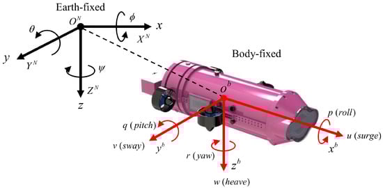
Figure 1.
Body-fixed and earth-fixed reference frames.
The 6-DoF equations of motion follow the framework established by Fossen [1]:
where, M is the inertia matrix, the sum of the rigid body inertia and added mass inertia : ; the Coriolis and centripetal matrix combines rigid body and added mass components: ; the damping matrix includes potential damping, skin friction, wave drift damping, and vortex shedding; and is the hydrostatic restoring force and moment vector.
2.1. Vehicle Kinematics
The 6-DoF kinematic equations for an underwater vehicle can be derived by expanding and into Equation (4). Here, represents the transformation matrix for linear velocity from the body-fixed frame to the earth-fixed frame, following the common -sequence used in navigation. represents the transformation matrix for the angular velocity vector.
2.2. Vehicle Dynamic
The proposed dynamic model of the underwater vehicle in this article is simplified based on the following assumptions:
- The vehicle is symmetrical port/starboard.
- Damping terms higher than second order are neglected.
- Buoyancy and gravity of the vehicle are equal.
- The center of buoyancy and gravity are vertically aligned on the body-fixed z-axis, i.e., , and .
- The vehicle moves at a low speed.
2.2.1. Rigid Body Dynamic
2.2.2. Hydrostatic Forces and Moments
Since we analyze forces and moments applied to the vehicle in the body-fixed coordinate system, represents the effect of weight and buoyancy transformed from the earth-fixed coordinate to the body-fixed coordinate. To further simplify the vehicle’s representation, let . The restoring forces and moments can then be expressed by Equation (8):
2.2.3. Hydrodynamic Forces and Moments
When moving in a fluid, the hydrodynamic forces acting on an underwater vehicle are generally comprised of three components: added mass-induced inertia forces, damping forces, and environmental disturbance forces. To develop an accurate hydrodynamic simulation model for an underwater vehicle (operating in deep sea or areas less affected by wind and waves), the assumption of as proposed by [1] is not adopted. The reason is, in real marine environments, there are often unexpected currents and wave influences. Furthermore, [49] demonstrated that the acceleration terms in the added mass matrix can be calculated with considerable precision using theoretical methods.
Typically, the added mass coefficients are assumed to be constant. The added mass terms are calculated using fluid kinetic energy theory. As the vehicle moves through a fluid, the surrounding fluid is displaced and then closes in behind the vehicle. This interaction passively generates added kinetic energy , where . This represents the kinetic energy possessed by the fluid due to the vehicle’s motion, which would not exist if the vehicle were stationary.
Our model enhances Abkowitz’s nonlinear model by incorporating truncated Taylor-series expansions for odd-order terms, following the approach of Fedyaevsky and Sobolev to alternate the third-order terms of Abkowitz’s model into second-order modulus. This adjustment is particularly suitable for low-speed field operations and simplifies parameter complexities. Additionally, we introduce cross-flow drag resulting from the coupling motion of sway and yaw, denoted as , , , and , following SNAME notation. These terms, derived from a 3D implementation of two 2D strip theory formulas, account for nonlinear damping forces from each hull section [50], aiding in handling currents not aligned with the heading . Fitting these formulas without integrals yields second-order terms, resembling a maneuvering model akin to that of Fedyaevsky and Sobolev. Cross-flow drag, as described in [11], refers to damping forces perpendicular to the x-axis resistance. Understanding and simulating cross-flow drag offer detailed insights into the mathematical model, potentially improving hydrodynamic performance, vehicle motion analysis, and state estimation accuracy. While many of these effects are relatively small, their inclusion can refine the model’s accuracy, although some may be ignored based on specific engineering considerations.
2.2.4. Thruster Forces and Moments
In the context of underwater vehicle dynamics, the force vector in Equation (3) primarily represents the thruster forces and any environmental forces acting on the vehicle. Neglecting environmental influences like wind, waves, and currents, is the thruster forces. This relationship is expressed as, , where B denotes the thrust distribution matrix, and represents the input forces vector of all the thrusters.
2.3. Six-DoF Nonlinear Equations of Motion
All the hydrodynamic parameters of AUV-shark are obtained from our previous work [51,52], with relevant physical parameters listed in Table 1. Compared to Fossen’s unsimplified vectorial model (non-symmetry, positive definite), our model, as shown in Equations (9)–(12), simplifies about the XOZ plane. Consequently, the hydrodynamic parameters in and can be reduced from 36 and 48 to 18 and 26, respectively. This reduction approximately halves the number of unknown hydrodynamic parameters, from 84 to 44.

Table 1.
Physical characteristics of AUV-shark.
As mentioned, compared to damping terms, added mass inertial terms are more accurately computed theoretically. Therefore, identifying damping terms has been the primary focus of hydrodynamic computation. In this paper, we will focus on identifying all 26 damping terms in , which encompass linear, nonlinear, and coupling effects.
3. Kalman Filter Hydrodynamic Parameters Identification
Mathematical models for underwater vehicles must incorporate realistic physical assumptions and simplifications. Model-based identification primarily targets damping terms with substantial errors, while identification methods based on nonlinear function fitting can more accurately capture underwater system characteristics. The selection of identification methods and the number of parameters greatly affect the accuracy of the identification results. In this section, the EKF algorithm for hydrodynamic parameter identification is introduced, with a focus on the damping terms in the underwater vehicle model.
3.1. Extended Kalman Filter
Real-world systems often exhibit nonlinear characteristics, necessitating the use of nonlinear approaches for state fusion algorithms. A prime example of such an algorithm is the EKF. The EKF linearizes nonlinear functions through a Taylor series expansion, ignoring higher-order terms to create a linearized model, thereby facilitating filtering for nonlinear systems. It balances the estimated values from the system model with the corrected values from actual measurements by utilizing a covariance matrix, which proportionally combines both to enhance data accuracy. The computational process for applying EKF to system identification follows [53]. First, it is necessary to obtain the discrete system and measurement equations:
where, represents the state vector, and denotes the measurement vector. and are zero mean Gaussian white system noise vector for process and measurement, respectively. The covariance matrices of the system noise and measurement noise are and , respectively. The Jacobian matrices for the system and measurement equations are indicated by and . The EKF algorithm involves three steps: initialization, time update, and measurement update, as detailed in [36].
3.2. Kalman Filter Setting
The augmented state space method utilized by [31,36] encounters convergence challenges in our application. Analysis reveals that continuous updating of the robot’s state variables within the state propagation equation, due to inconsistencies between computed and predicted results, acts as an unnecessary filter for hydrodynamic parameter identification. This results in the algorithm compensating for prediction errors, leading to premature convergence of non-hydrodynamic state variables. Consequently, this hinders the accurate convergence of hydrodynamic parameters and increases the likelihood of divergence. This issue is particularly pronounced when dealing with a large number of hydrodynamic parameters. In this study, we aim to identify a 6-DoF system with up to 26 hydrodynamic parameters, which exacerbates the limitations of the Kalman filter.
To address these convergence challenges, the problem is simplified by following the approach outlined in [54]. We define the state vector x as a column vector consisting of 26 damping hydrodynamic parameters to be identified and the observation vector y as the vehicle’s linear velocity, angular velocity, position, and attitude. To derive the discrete system and measurement equations, we employ numerical integration techniques like the forward Euler method, backward Euler method, and fourth-order Runge–Kutta (4th-RK). Initially, we selected the 4th-RK due to its high accuracy and convergence ability. However, its complexity, resulting from the combination of four slopes over four-time steps, leads to a complicated state space update equation and a large, intricate Jacobian matrix in the EKF (a 38 by 38 matrix with some complex elements), making the process very time-consuming. Consequently, to compromise between computational accuracy and efficiency, we opted for the backward Euler method instead.
According to Equation (3), the derivative of the speed vector can be derived as follows:
To derive the system measurement equation, we substitute Equations (2) and (16) into Equation (18). As a result, the Jacobian matrix F becomes an identity matrix, and the Jacobian matrix H becomes a 12 by 26 matrix. During sea trial, GPS signals attenuate rapidly in water, making accurate horizontal positioning for underwater vehicles unattainable. Therefore, the position elements x and y of observation vector are set to zero, resulting in .
where is the state vector of hydrodynamic parameters, is the observation interval, and represents the processing time step.
The process noise covariance matrix and measurement noise covariance matrix are both set as constant matrices, as shown in Equations (20) and (21):
The values represent standard deviations. The standard deviation in the measurement noise covariance matrix R can be calculated by sampling data from different sensors. However, determining the standard deviations in the process noise covariance matrix Q is more complex. We initialize Q as an identity matrix I and adjust its diagonal element according to the sampling time step length, hydrodynamic parameter magnitude, and identification results. As noted by [55], there are no direct methods to accurately determine the values of the process noise covariance matrix Q. Hence, the values of Q are usually based on experiences and are specific to the context, lacking transferability and generalizability.
4. Long Short-Term Memory System Identification
Except for hydrodynamic parameter identification, there are other ways to obtain an underwater vehicle model, like analytical and semi-empirical(ASE) [56], and nonlinear regression [37]. Here, a special recurrent neural network, LSTM, is introduced. The LSTM network uses time-series information to capture the complex relation between input and output variables, which perfectly aligns with the complex dynamics equations of the underwater vehicle. Unlike traditional neural networks, LSTM are specifically designed to handle sequential data using a cell structure chain-like loop, enabling LSTM to memorize temporal features with reduced complexity. This makes LSTM-based methods widely used in time-series analysis. To understand the mechanism of LSTM network, we need to start from the core unit—the LSTM cell—which acts as the regulator of information flow within the network and plays a crucial role in managing its internal memory. Equation (22) shows the mathematical design of the cell [57]:
An LSTM cell is capable of addressing the long-term dependency problem by changing the cell state according to its forgot gate, input gate, and output gate in four steps. The first step is to discard unwanted information, which is realized by a sigmoid layer output f that ranges from 0 to 1. The second step is to include new cell state information by a selector i that chooses what information to update and a hyperbolic tangent function output that relates to the potential new cell state. Then combining above three outputs to obtain the updated cell state c. Finally, we can derive the filtered cell output after a scaling layer from current input , last output , and c. W denotes different weight matrixes, b is bias vector, and ⊙ denotes the elementwise product. The subscript t denotes time step, and the superscript l denotes the lth LSTM layer. By interconnecting LSTM cells, we create an LSTM layer. Stacking LSTM layers alongside other hidden layers, such as fully connected and dropout layers, allows us to construct deep LSTM networks.
4.1. LSTM Network Structure
Space robots benefit significantly from a 6-DoF dynamic model, offering superior controllability compared to limited actuator designs. This comprehensive controllability translates to enhanced robustness in tasks requiring precise manipulation and positioning. Additionally, 6-DoF non-parametric models facilitate the development of algorithms for synthetic fault diagnosis and dead reckoning, leading to improved mission success rates. Inspired by these benefits, a deep LSTM network is proposed for identifying the coupled 6-DoF nonlinear underwater vehicle model. This approach stands in contrast to underactuated models, such as the horizontal models presented in [41,58]. Since there are no unknown terms in the vehicle’s kinematics equation ( can be observed) and Equation (2) is brief and clear, we simply consider the dynamics of vehicle. As Equation (16) shows, the dynamic features can be seen as a multi-input multi-output nonlinear function, as shown in Equation (23):
According to Equation (23), our dynamic system utilizes 18 input variables, including velocity, position, attitude, control forces, and moments, to predict the system’s 6-dimensional speed derivatives. Notably, only is an independent variable, whereas all other terms are measurable. After developing a deep LSTM structure, the sequence data used for prediction should be prepared first. The required dataset contains both input and output data. Following the principles of LSTM, the input data must be a three-dimensional array in the form of samples, time steps, and features [59]. Samples represent the number of time sequences from different operations, with each sample corresponding to one sequence. Time steps denote the span of observation in a specific sample sequence, with each time step representing one step length. Features indicate the number of observations, with each feature corresponding to one observed quantity. Similarly, the output data has the same array structure. The LSTM model typically has eighteen inputs and six outputs, meaning the features of the input data and output data are 18 and 6, respectively. The operating principle of LSTM system identification with established features is illustrated in Figure 2. Selecting the number of samples and time steps is complex and depends on the experiment type, desired model accuracy, sensor data update frequency, and expected training duration. We will discuss samples and time steps further in data acquisition section.
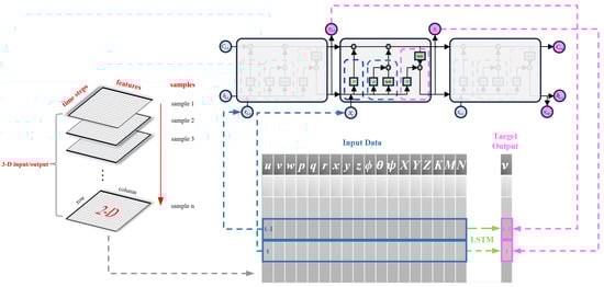
Figure 2.
Schematic diagram of Long Short-Term Memory (LSTM) data processing. Each plane stacked on the left represents a sampled maneuver trial reshaped into the desired format. The LSTM cell is visualized using distinct colors to represent its gates: forget gate (navy blue), input gate (dark blue), and output gate (magenta).
Our LSTM network architecture consists of two LSTM layers, two fully connected (FC) layers, and several dropout modules, as illustrated in Figure 3. The final fully connected layer employs a linear activation function to directly output the required values. Each intermediate layer allows for independent hyperparameter tuning, which significantly affects the recognition performance on a given dataset. The optimization of these hyperparameters directly influences the system’s recognition performance. Currently, the LSTM network is trained exclusively using simulation data, which includes four samples for the training set, one for the validation set, and one for the test set. Due to the limited learnable dynamic features in the simulated dataset compared to the variable dynamics of sea trials, the number of units in the LSTM layers has been increased to 300, with a corresponding dropout rate of 5%. The fully connected layers also have 300 units each. To ensure the output aligns with the required six-degrees-of-freedom information, the final fully connected layer is configured with six neurons. We use the coefficient of determination () to quantify the model’s prediction accuracy. The metric can be viewed as an loss function normalized by the variance of the true values, essentially measures the model’s ability to fit the data and predict unseen examples. During training, the swiftly rise above 0.95 after a few dozens of epochs, demonstrating that our model maintains excellent tracking capability.
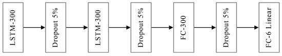
Figure 3.
Architectures of LSTM networks.
4.2. Dataset Acquisition
The dataset is one of the critical factors influencing the model’s prediction accuracy. It must adequately capture the unique coupling and nonlinearity characteristics of underwater vehicle. To construct a dataset encompassing a wide range of system characteristics, we run kinds of simulation experiments including acceleration-deceleration test, turning test, spiral test, zigzag test, variable-period sinusoidal input test, and 3-2-1-1 test. It has been proved that the zigzag maneuver experiments with varying control values contain more dynamic characteristics [60]. Compared with standard maneuver dataset, a dataset including zigzag tests can memorize and provide essential information about multi-DoF coupling and nonlinearity needed in identification. In addition, an appropriate dataset can alleviate the issue of parameter drift caused by collinearity of independent variables in data. We also use the 3-2-1-1 method proposed by [61], which was originally used for aircraft parameter identification. The meaning of 3-2-1-1 is that the input variable should be separated into four proportional periods in length of 3, 2, 1, and 1, and the sign of input changes after every period. It is a commonly employed technique due to its capability to stimulate the comprehensive frequency spectrum of the system’s dynamic response. Similar to the 3-2-1-1 test, the sinusoidal test aims to expand the state space response of sampled data by varying the amplitude and period. The findings of [38,41] even suggest that solely conducting the sinusoidal experiment suffices to create a high-performing LSTM dataset. In summary, various types of experiments are required to establish the dataset. The specific experimental designs are detailed in Table 2.
Table 2.
AUV shark design of experiments.
In this study, we collected five time-series samples for the dataset, each encompassing all experimental types. To ensure integration accuracy, we set the sampling frequency to 20 Hz and the sampling time to 2500 s. Each sample contains 50,000 points, resulting in three-dimensional input–output datasets of [5, 50,000, 18] and [5, 50,000, 6]. The dataset was split 80–20% into training (four samples) and validation (one sample) sets. Before each training iteration, we randomly shuffled the samples to enhance the diversity of temporal information and prevent the model from overfitting to specific sequences. Additionally, we designed a test set with a sampling duration of up to 2000 s to reflect real-world operational scenarios, including straight-line navigation, spiral ascents and descents, and yaw movements. The test set’s numerical configuration differs from the training and validation sets, which can be used to effectively demonstrate the LSTM’s ability to learn underwater vehicle dynamics and predict performance.
4.3. LSTM Dead Reckoning
A good way to evaluate the performance of the LSTM model is by using it to predict position through the DR method. According to [62], the main sources of error in DR are water currents. For our purposes, we assume operations occur in still water conditions. However, when estimating NED position using predicted with DR, the results show significant time delays and drift errors after double integration. This undesired bias primarily arises from the continuous error accumulation in . While the output preserves all motion features, they are distorted by incorrect attitude estimates. Additionally, obtaining accurate body-fixed acceleration data is challenging [63]. We typically derive by differentiating the velocity provided by DVL or using IMU data. Both methods have significant drawbacks: differentiating velocity amplifies sensor noise and heavily depends on sampling frequency, while IMU data suffer from considerable noise and drift due to temperature and time. Given these issues, we use Equation (24) instead of Equation (23) to address these challenges.
Here, k represents the time step, is the time interval. By applying Equation (24) to LSTM-based system identification, we can predict the velocity at time step given the input at , enabling real-time speed prediction. The discrete velocity recursion formula reduces one integration step, significantly diminishing drift and time delay in position reckoning, and helps prevent error accumulation from integration. However, in theory, the slight discrepancies in LSTM predictions can be amplified through the intrinsic coupling relationship in the coordinate transformation matrix , potentially causing divergence in the position and orientation . This issue is particularly evident when calculating the attitude . In practice, even small non-zero errors in predicted angular velocities can, over time, lead to significant deviations in angles due to prolonged integration. Such deviations, similar to the effects of uncertainty in hydrodynamic parameters, cause non-zero off-diagonal elements in that should be zero near zero values. This introduces unintended coupling in the calculation of position acceleration, ultimately leading to attitude instability. The result is oscillatory divergence in roll and pitch angles, deviating from the true trajectory. Therefore, achieving accurate dead reckoning requires more reliable methods for obtaining precise attitude. To address this, we obtain using the NECF method proposed by [45] and then use the estimated attitude to calculate the transformation matrix . This attitude estimation method, which relies on filtered acceleration and horizontal magnetic field data, is especially effective for underwater vehicles. The most influential factor affecting NECF is magnetic distortion, which arises from hard and soft iron effects as well as non-horizontal vibrations caused by hydrodynamics, resulting in fluctuating inclined planar magnetic field. To address this, we apply the random sample consensus (RANSAC) algorithm [64] during the magnetic data plane fitting phase to eliminate outliers.
Assuming reliable is available, we use the backward Euler discrete integration expressed in Equation (25) as DR method. Alternative methods, such as trapezoidal integration or Simpson’s rule, are also viable. The optimal method should be chosen by balancing computational efficiency and precision.
5. Simulation Evaluation and Experiment Setup
The proposed EKF identification approach and LSTM architecture are both tested and compared with the previously designed 6-DoF numerical model of the AUV shark. EKF and LSTM utilize different datasets generated by substituting simulation into Equation (14), with the 4th-RK integration method used to solve the system state space ordinary differential equation. In the LSTM dataset, the amplitude and period of each input variable change with every sample to broaden the sampled state space. Notably, the AUV shark is an underactuated vehicle, allowing control in only 4-DoF, which means we deliberately minimize the lateral force Y and vertical moment M. However, this does not imply that the vehicle should not move in all degrees of freedom, on the contrary, we encourage as many maneuvering situations as possible. Because of limited motility, the derived datasets lack certain active motion characteristics, leading to non-negligible misalignment in v, y, q, and sometimes. Although this issue can be mitigated by introducing observable additional current disturbances, this method is not discussed in this article. The validation of our study depends on the sensors installed on AUV-Shark, with their specifications outlined in Table 3. These sensors are synchronized with the update rate of DVL, operating at approximately 10 Hz, corresponding to the bottom track altitude.
Table 3.
Sensor specification of AUV shark.
5.1. Model Performance
Given the high cost of underwater operating systems, it is crucial to avoid unnecessary losses and enhance the accuracy of predicting the motion state of underwater vehicles. This necessitates a dynamic model that closely reflects actual physical characteristics. There are various physical models for underwater vehicles based on different assumptions, such as the Nomoto model, Whitcomb–McFarland model [27], Gertler–Hagen model, and Fedyaevsky–Sobolev (FS) model [50]. This paper focuses on analyzing and comparing the proposed port/starboard model with the second-order FS hydrodynamic model. The FS model, based on three-plane symmetry, is a commonly used model that requires only eighteen hydrodynamic parameters, including six acceleration terms and twelve damping terms, all of which are distributed along the diagonal of the parameter matrix.
The hydrodynamic parameters derived from CFD simulations and empirical formulas can be applied to Equation (14) to develop models that adhere to these simplified constraints. By employing 4th-RK, the model’s stability and dynamic behavior can be verified. As illustrated in Figure 4, both systems stabilize within 15 s under the initial conditions , without accounting for external disturbances such as currents, waves, and wind.
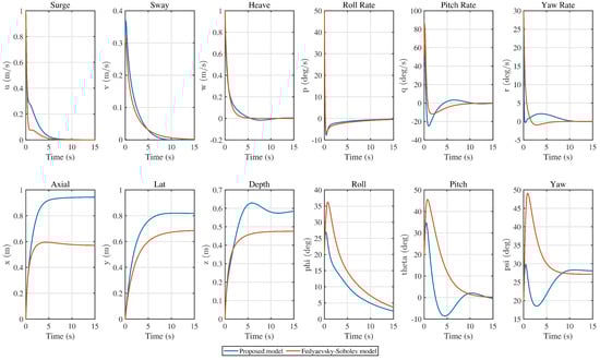
Figure 4.
Six-DoF nonlinear coupled model simulation result.
The comparison between the two models reveals significant differences. The weakly coupled model, based on the three-plane symmetry assumption, differs markedly from the strongly coupled model proposed in this paper. For instance, in the x-direction displacement, the rapid decline of the strongly coupled model slows down after . This is because the negative angular rate q and positive depth speed w at this moment in the AUV simulation model cause the velocity u to have a changing component due to and . When combined with the damping matrix , this leads to complex coupling effects. However, this critical phenomenon is not captured in the weakly coupled FS model, which lacks sufficient coupling effects to account for the relationships between different DoF, thereby missing the actual motion changes along the x-direction. Similar situations can also be observed in the depth turning point at , caused by pitch and heave coupling, and oscillatory behavior in pitch and yaw directions due to off-diagonal hydrodynamic parameters.
Hence, the strongly coupled model, which assumes only port/starboard symmetry, better captures the actual motion coupling dynamics and provides more valuable simulation data. In contrast, weakly coupled models like the FS model have greater errors. The simulation results closely match actual experimental phenomena, particularly in surge, heave, and heading directions, accurately reflecting the dynamic characteristics of the underwater robot in a controlled environment.
5.2. EKF Hydrodynamic Parameters Identification
Achieving precise accuracy for all damping terms can be challenging. To facilitate EKF convergence, we implemented phases involving one or two movements lasting around 20 s each. Without time constraints for offline computation, we set the total sampling duration to 190 s. The EKF-identified results are depicted in Figure 5 and summarized in Table 4. In most estimations, the EKF maintains relatively small absolute error and exhibits high reliability in identifying hydrodynamic parameters compared to CFD results. This enables experimental tests using EKF-identified parameters instead of traditional towing tank measurements, significantly reducing time and cost. Additionally, EKF-derived linear velocity can train the LSTM model and access sensor data.
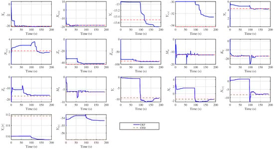
Figure 5.
Extended Kalman Filter (EKF)-estimated hydrodynamic coefficients. Disregard parameters near zero; certain coefficients associated with sway velocity fail to converge initially due to model properties.
Table 4.
Error analysis of EKF-predicted hydrodynamic damping parameters.
Analysis of the EKF identification results reveals major errors in the hydrodynamic parameters associated with lateral velocity v and yaw rate r. These errors predominantly arise from uncertainties regarding the sign of the parameters rather than values. Notably, when different hydrodynamic parameters affecting the same DoF exhibit opposite signs, their respective impacts on the system’s dynamic characteristics contradict each other, exacerbating the nonlinear coupling between the v and r DoF in underwater vehicle. Despite efforts to minimize prediction errors, the EKF algorithm often struggles to simultaneously track all converging factors, leading to substantial deviations or even divergence in the identified hydrodynamic parameters. Furthermore, this challenge is particularly pronounced for hydrodynamic parameters approaching zero. Leveraging both model outputs and sensor measurements, the Kalman filter enables underwater vehicle to compensate for multiple sensor data, predict unknown variables, and impose constraints. Currently, apart from , most hydrodynamic parameters exhibit promising convergence trends, converging to within 10% steady-state error after appropriate adjustments to the process covariance matrix Q. Parameters such as , , and demonstrate rapid convergence, minimal error, and negligible oscillations, indicating less coupling. In contrast, parameters showing slow convergence, pronounced oscillations, and fluctuating errors suggest significant internal coupling and pose challenges for convergence. Importantly, some convergence outcomes of the system identification method based on the Kalman filter are heavily influenced by the Q matrix, for which there is no universally applicable determination method. During sensitivity analysis, sway and yaw-related damping coefficients were found to be more sensitive than other DoF. Specifically, coefficients such as , , , , and are difficult to match to their true values due to their sensitivity to velocity changes, covariance matrix variations, and complex internal coupling effects. To enhance the accuracy of these parameters, their initial values were set close to known values, and the proportion of single-DoF maneuvering data in the samples was increased.
5.3. LSTM Model Validation
During training, we use a batch size of 1 for independent gradient calculation and parameter updates, theoretically supporting online identification. The LSTM and FC layer weights are initialized with the Glorot uniform initializer, and biases are set to zero. We employ the Adam optimizer to speed up convergence, training for 500 epochs with a learning rate of 0.001 and decay of 0.0001 to minimize the mean squared error (MSE) loss function. Data is pre-scaled to the [−1, 1] range and shuffled before each epoch to reduce variance. The model’s performance is validated after each epoch using the validation set. Training is conducted on a Linux PC with a 4-core Intel Core i7-4790K CPU and an NVIDIA GTX 1080Ti GPU using TensorFlow and the Keras library.
The predicted 6-DoF velocity information from the proposed deep LSTM network architecture is illustrated in Figure 6. The model’s accuracy and robustness are further demonstrated through the normalized error distribution of 40,000 predicted data points, as shown in Figure 7. Most velocity prediction errors are centered around zero, with larger errors being relatively rare. This indicates that the LSTM effectively captures the complex dynamics of underwater vehicle, showing great promise for state prediction in autonomous underwater vehicles. However, it is important to note that the current model, which trained on the existing dataset, exhibits major errors in angular velocity predictions due to a lack of corresponding features. Despite adhering to the experimental design process for system identification of underwater vehicle, the model still struggles with angular velocity accuracy. Angular velocity predictions contain more outliers than linear velocity predictions. Inaccurate angular rate predictions by the LSTM can significantly impact the accuracy of dead reckoning, leading to quicker deviations from the true position during long-term complex missions.
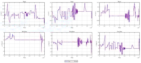
Figure 6.
LSTM prediction results of 6-DoF velocity.
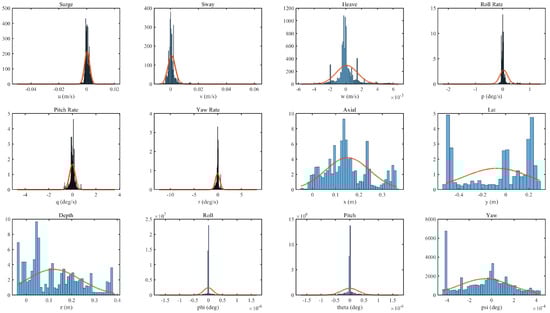
Figure 7.
Error normal distribution of test dataset.
While pure LSTM-based dead reckoning provides sufficient short-term accuracy, it cannot compensate for the unbounded errors introduced by continuous integration. When LSTM-predicted angular velocities are used in calculations, the predictions begin to diverge around 400 s, eventually resulting in significant errors, aligning with our analysis. A similar issue is highlighted in [65], where using only the LSTM output for navigation estimation causes rapid localization error growth during rotation on the horizontal plane. This error accumulation becomes significant during long-duration and long-distance operations, especially with frequent steering maneuvers. Therefore, this paper seeks a solution to mitigate integration errors in pure LSTM-based methods. To improve prediction precision, one solution is to increase the amount of training data related to specific maneuvering tests. However, this approach could burden computational efficiency. Therefore, we opted to use NECF to estimate attitude directly. The LSTM-predicted can still serve as a backup metric in case of sensor failure or overwhelming magnetic distortion. Additionally, when combined with the EKF state space equation, the LSTM can be viewed as another reliable data source for velocity prediction.
To provide NECF attitude estimation for DR, we implement a test using the Xsens MTi-G-710 IMU. To evaluate the performance of attitude estimation in simulated underwater operations, we rotated the x-axis of a magnetometer through a full circle, starting and ending aligned with the magnetic north, on a plane with non-horizontal rotations less than . As shown in Figure 8, the estimated yaw angle matches the true value, with deviations toward magnetic north at the beginning and end mostly under .
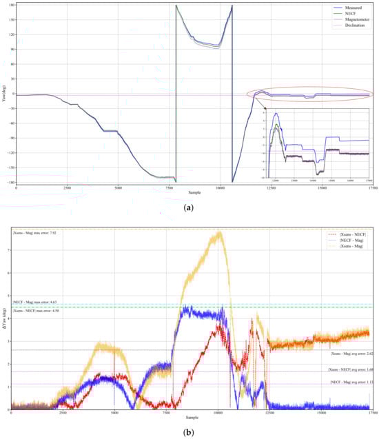
Figure 8.
Schematics of Nonlinear Explicit Complementary Filter (NECF) yaw estimation. (a) Estimates of NECF, IMU, and magnetic data about yaw angle in true north frame (NED). (b) Yaw error comparison.
Notably, the magnetic declination has an uncertainty of according to the World Magnetic Model (WMM, 2019–2024). The maximum error occurs after a rapid turn of the magnetometer, caused by the filter’s inherent delay. Designed for stability and robustness, the filter responds slowly to rapid changes. Despite of this, the tested average error of is sufficient for most underwater operations where the vehicle typically moves slowly and steadily. The applied filter demonstrates superior corrective ability compared to the Xsens magnetic field filter. Both filters lag behind the magnetic field during rapid changes, but the applied filter quickly corrects the error based on a pre-designed regulator that relates the estimated direction to the fixed magnetic north. In contrast, the IMU filter shows an irreversible bias after a significant jump of . When the vehicle returns to the original position, the IMU’s filter maintains a bias of with a rising trend, while NECF corrects the error to near zero as soon as the rotation rate drops to a manageable range. This indicates that the applied filter has a superior ability to correct errors caused by swift turns and magnetic distortion.
For the preliminary validation of the NECF-aided LSTM-based dead reckoning method, we assume the attitude angles are observable and accurate. The position estimation results, using Equations (24) and (25), are shown in Figure 9. The predicted position closely matches the true path. The box plot illustrates error distributions for each specific direction, with low median errors across all three axes, signifying precise dead reckoning. Compact box structures indicate concentrated errors with narrow whiskers, highlighting the accuracy of position estimation. This study has validated the feasibility of a DR method that does not rely on positioning sensors like DVL, sonar, or GPS, using the LSTM system identification algorithm, IMU, and a magnetometer. In an undisturbed simulation environment, the system successfully maintained position prediction errors within 1 m across three degrees of freedom over a continuous operation of 2000 s. The predicted positions closely match the actual positions, with the largest errors typically occurring in the surge and sway directions. Depth errors are usually minimal compared to the overall depth change and can be considered negligible with depth gauge compensation. Errors in x and y are primarily caused by inaccuracies in yaw angle and the surge and sway velocities u and v. Over extended periods, position prediction may diverge due to fluctuations in these variables.
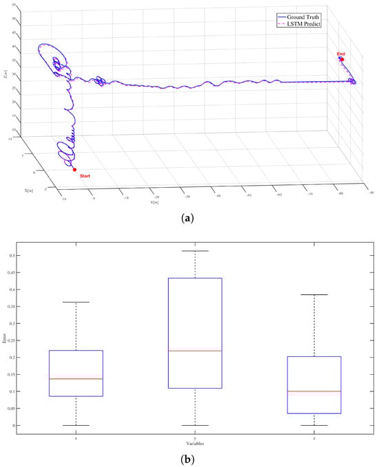
Figure 9.
LSTM-based AUV shark position prediction result. (a) AUV 3D trajectory. (b) Position error box diagram.
Velocity and attitude estimation are critical for underwater navigation via dead reckoning, particularly when positioning sensors are malfunction or unavailable. The NECF method employs acceleration filtering, magnetometer calibration, correction term optimization, and dynamic weighting to enhance attitude estimation performance cost-effectively. Experiments demonstrate that NECF outperforms Xsens in accuracy, offering superior resistance to magnetic interference and robustness. NECF resolves angle divergence in LSTM-based velocity prediction models for passive localization, validating the effectiveness of the proposed NECF-aided LSTM dead reckoning method for navigation.
6. Conclusions
This study provides a comprehensive solution to the challenges of system identification and navigation for underwater vehicles by integrating advanced dynamic modeling, parameter identification, data-driven system identification, and attitude estimation-based navigation techniques. A novel 6-DoF fully coupled nonlinear dynamic model is derived from the Fedyaevsky–Sobolev framework, incorporates cross-flow drag effects in sway and yaw while considering port-starboard symmetry. Unlike standard models, it avoids relying on low-precision assumptions and accurately captures the coupled dynamics of underactuated, finless, and low-speed AUVs, showing improved stability and controllability. Validation is carried out using benchmark CFD simulation data. A model-based EKF hydrodynamic parameter identification method is developed, enabling estimation of all damping coefficients using sensor measurements without specialized equipment. This approach enhances stability and accuracy by extracting system state variables from the augmented state vector while excluding horizontal positions prone to significant errors, thus avoiding divergence in parameter estimation. This approach provides a reliable validation framework for CFD simulations. Additionally, a non-parametric deep LSTM network is introduced for navigation without DVL. By focusing on input–output relationships, the LSTM model eliminates the need for complex hydrodynamics and ideal assumptions. A generalized dataset construction method is proposed to capture the unique coupling and nonlinear dynamics of underwater vehicles. This method integrates various experimental scenarios, including acceleration-deceleration, turning, spiral, zigzag, sinusoidal, and 3-2-1-1 maneuvers, ensuring effective dataset coverage even with limited samples. To address angular velocity error accumulation and position divergence in LSTM-based dead reckoning, an NECF-aided navigation method is proposed. By integrating IMU, magnetometer, and the LSTM model, this method enables robust attitude estimation and passive localization in GPS-denied or sensor failure conditions, achieving favorable accuracy over 2000 s. This paper highlights the potential for parameter identification without reliance on towing tank, planar motion mechanism, and rotating arm experiments, as well as navigation without localization sensors, which are particularly beneficial for small underwater vehicles with extended mission durations and demanding maneuvering needs. Future works will focus on online applications of LSTM to adjust estimated models adaptively, and integrate EKF, LSTM, and NECF for a reliable navigation system without sensor reliance.
Author Contributions
Conceptualization, C.L. and D.Z.; methodology, C.L.; software, C.L. and Z.H.; validation, C.L., Z.H. and D.Z.; formal analysis, C.L.; investigation, C.L. and D.Z.; resources, X.W.; data curation, C.L.; writing—original draft preparation, C.L.; writing—review and editing, D.Z. and X.W.; visualization, C.L.; supervision, X.W.; project administration, X.W.; funding acquisition, X.W. All authors have read and agreed to the published version of the manuscript.
Funding
The work is supported by the Shenzhen Science and Technology Program (JSGG20211029095205007), the Shenzhen Science and Technology Major Program (KJZD20231023100459001) and the Guangdong Provincial Key Laboratory of Intelligent Morphing Mechanisms and Adaptive Robotics Program (2023B1212010005).
Institutional Review Board Statement
Not applicable.
Informed Consent Statement
Not applicable.
Data Availability Statement
The data are available upon request.
Conflicts of Interest
The authors declare no conflicts of interest.
References
- Fossen, T.I. Guidance and Control of Ocean Vehicles. Ph.D. Thesis, University of Trondheim, Trondheim, Norway, 1999. [Google Scholar]
- Abkowitz, M.A. Lectures on Ship Hydrodynamics–Steering and Manoeuvrability; Technical Report; National Academy of Sciences: Washington, DC, USA, 1964. [Google Scholar]
- Chislett, M.; Strom-Tejsen, J. Planar motion mechanism tests and full-scale steering and manoeuvring predictions for a mariner class vessel. Int. Shipbuild. Prog. 1965, 12, 201–224. [Google Scholar] [CrossRef]
- Yasukawa, H.; Yoshimura, Y. Introduction of MMG standard method for ship maneuvering predictions. J. Mar. Sci. Technol. 2015, 20, 37–52. [Google Scholar] [CrossRef]
- Gertier, M.; Hagen, G.R. Standard Equations of Motion for Submarine Simulation; Technical Report; Naval Ship Research and Development Center: Bethesda, MD, USA, 1967. [Google Scholar]
- Fu, J.; Zhou, H.; Zhang, X.; Wen, H.; Yao, B.; Lian, L. A unified switching dynamic modeling of multi-mode underwater vehicle. Ocean. Eng. 2023, 278, 114359. [Google Scholar] [CrossRef]
- Kinsey, J.C.; Yang, Q.; Howland, J.C. Nonlinear dynamic model-based state estimators for underwater navigation of remotely operated vehicles. IEEE Trans. Control. Syst. Technol. 2014, 22, 1845–1854. [Google Scholar] [CrossRef]
- Arnold, S.; Medagoda, L. Robust model-aided inertial localization for autonomous underwater vehicles. In Proceedings of the 2018 IEEE international conference on robotics and automation (ICRA), Brisbane, Australia, 21–25 May 2018; pp. 4889–4896. [Google Scholar]
- Lv, P.F.; He, B.; Guo, J.; Shen, Y.; Yan, T.H.; Sha, Q.X. Underwater navigation methodology based on intelligent velocity model for standard AUV. Ocean. Eng. 2020, 202, 107073. [Google Scholar] [CrossRef]
- Prestero, T.T.J. Verification of a Six-Degree of Freedom Simulation Model for the REMUS Autonomous Underwater Vehicle. Ph.D. Thesis, Massachusetts Institute of Technology, Cambridge, MA, USA, 2001. [Google Scholar]
- Yang, C. Modular Modeling and Control for Autonomous Underwater Vehicle (AUV). 2008. Available online: https://core.ac.uk/reader/48625100 (accessed on 25 December 2024).
- Skjetne, R.; Smogeli, Ø.; Fossen, T.I. Modeling, identification, and adaptive maneuvering of Cybership II: A complete design with experiments. IFAC Proc. Vol. 2004, 37, 203–208. [Google Scholar] [CrossRef]
- Park, J.; Rhee, S.H.; Yoon, H.K.; Lee, S.; Seo, J. Effects of a propulsor on the maneuverability of an autonomous underwater vehicle in vertical planar motion mechanism tests. Appl. Ocean. Res. 2020, 103, 102340. [Google Scholar] [CrossRef]
- Oliverira, P.; Silvestre, C.; Aguiar, P.; Pascoal, A. Guidance and control of the SIRENE underwater vehicle: From system design to tests at sea. In Proceedings of the IEEE Oceanic Engineering Society. OCEANS’98. Conference Proceedings (Cat. No. 98CH36259), Nice, France, 28 September–1 October 1998; Volume 2, pp. 1043–1048. [Google Scholar]
- Goheen, K.; Jefferys, E. The application of alternative modelling techniques to ROV dynamics. In Proceedings of the IEEE International Conference on Robotics and Automation, Cincinnati, OH, USA, 13–18 May 1990; pp. 1302–1309. [Google Scholar]
- Marco, D.B.; Martins, A.; Healey, A.J. Surge motion parameter identification for the NPS Phoenix AUV. Proc. Int. Adv. Robot. Program IARP 1998, 98, 197–210. [Google Scholar]
- Ziani-Cherif, S.; Lebret, G.; Perrier, M. Identification and control of a submarine vehicle. IFAC Proc. Vol. 1997, 30, 307–312. [Google Scholar] [CrossRef]
- Alessandri, A.; Caccia, M.; Indiveri, G.; Veruggio, G. Application of LS and EKF techniques to the identification of underwater vehicles. In Proceedings of the 1998 IEEE International Conference on Control Applications (Cat. No. 98CH36104), Trieste, Italy, 4 September 1998; Volume 2, pp. 1084–1088. [Google Scholar]
- Indiveri, G. Modelling and identification of underwater robotic systems. Comput. Sci. 1998. [Google Scholar]
- Caccia, M.; Indiveri, G.; Veruggio, G. Modeling and identification of open-frame variable configuration unmanned underwater vehicles. IEEE J. Ocean. Eng. 2000, 25, 227–240. [Google Scholar] [CrossRef]
- Smallwood, D.A.; Whitcomb, L.L. Preliminary experiments in the adaptive identification of dynamically positioned underwater robotic vehicles. In Proceedings of the Proceedings 2001 IEEE/RSJ International Conference on Intelligent Robots and Systems. Expanding the Societal Role of Robotics in the the Next Millennium (Cat. No. 01CH37180), Maui, HI, USA, 29 October–3 November 2001; Volume 4, pp. 1803–1810. [Google Scholar]
- Van De Ven, P.W.; Johansen, T.A.; Sørensen, A.J.; Flanagan, C.; Toal, D. Neural network augmented identification of underwater vehicle models. Control. Eng. Pract. 2007, 15, 715–725. [Google Scholar] [CrossRef]
- Martin, S.C. Advances in Six-Degree-of-Freedom Dynamics and Control of Underwater Vehicles. Ph.D. Thesis, Johns Hopkins University, Baltimore, MD, USA, 2008. [Google Scholar]
- Ramirez, W.A.; Kocijan, J.; Leong, Z.Q.; Nguyen, H.D.; Jayasinghe, S.G. Dynamic system identification of underwater vehicles using multi-output Gaussian processes. Int. J. Autom. Comput. 2021, 18, 681–693. [Google Scholar] [CrossRef]
- Karras, G.C.; Loizou, S.G.; Kyriakopoulos, K.J. Towards semi-autonomous operation of under-actuated underwater vehicles: Sensor fusion, on-line identification and visual servo control. Auton. Robot. 2011, 31, 67–86. [Google Scholar] [CrossRef]
- Xu, F.; Zou, Z.J.; Yin, J.C.; Cao, J. Identification modeling of underwater vehicles’ nonlinear dynamics based on support vector machines. Ocean. Eng. 2013, 67, 68–76. [Google Scholar] [CrossRef]
- McFarland, C.J.; Whitcomb, L.L. Comparative experimental evaluation of a new adaptive identifier for underwater vehicles. In Proceedings of the 2013 IEEE International Conference on Robotics and Automation, Karlsruhe, Germany, 6–10 May 2013; pp. 4614–4620. [Google Scholar]
- Cardenas, P.; de Barros, E.A. Estimation of AUV hydrodynamic coefficients using analytical and system identification approaches. IEEE J. Ocean. Eng. 2019, 45, 1157–1176. [Google Scholar] [CrossRef]
- An, X.K.; Du, L.; Jiang, F.; Zhang, Y.J.; Deng, Z.C.; Kurths, J. A few-shot identification method for stochastic dynamical systems based on residual multipeaks adaptive sampling. Chaos Interdiscip. J. Nonlinear Sci. 2024, 34, 073118. [Google Scholar] [CrossRef]
- Sabet, M.T.; Sarhadi, P.; Zarini, M. Extended and Unscented Kalman filters for parameter estimation of an autonomous underwater vehicle. Ocean. Eng. 2014, 91, 329–339. [Google Scholar] [CrossRef]
- Sabet, M.T.; Daniali, H.M.; Fathi, A.; Alizadeh, E. Identification of an autonomous underwater vehicle hydrodynamic model using the extended, cubature, and transformed unscented Kalman filter. IEEE J. Ocean. Eng. 2017, 43, 457–467. [Google Scholar] [CrossRef]
- Ahmad, S. Linear and nonlinear system identification techniques for modelling of a remotely operated underwater vehicle. Int. J. Model. Identif. Control. 2015, 24, 75–87. [Google Scholar] [CrossRef]
- Luo, W.; Guedes Soares, C.; Zou, Z. Parameter identification of ship maneuvering model based on support vector machines and particle swarm optimization. J. Offshore Mech. Arct. Eng. 2016, 138, 031101. [Google Scholar] [CrossRef]
- Wu, N.L.; Wang, X.Y.; Ge, T.; Wu, C.; Yang, R. Parametric identification and structure searching for underwater vehicle model using symbolic regression. J. Mar. Sci. Technol. 2017, 22, 51–60. [Google Scholar] [CrossRef]
- Shariati, H.; Moosavi, H.; Danesh, M. Application of particle filter combined with extended Kalman filter in model identification of an autonomous underwater vehicle based on experimental data. Appl. Ocean. Res. 2019, 82, 32–40. [Google Scholar] [CrossRef]
- Deng, F.; Levi, C.; Yin, H.; Duan, M. Identification of an Autonomous Underwater Vehicle hydrodynamic model using three Kalman filters. Ocean. Eng. 2021, 229, 108962. [Google Scholar] [CrossRef]
- Wehbe, B.; Hildebrandt, M.; Kirchner, F. Experimental evaluation of various machine learning regression methods for model identification of autonomous underwater vehicles. In Proceedings of the 2017 IEEE International Conference on Robotics and Automation (ICRA), Singapore, 29 May–3 June 2017; pp. 4885–4890. [Google Scholar]
- Wehbe, B.; Arriaga, O.; Krell, M.M.; Kirchner, F. Learning of Multi-Context Models for Autonomous Underwater Vehicles. In Proceedings of the 2018 IEEE/OES Autonomous Underwater Vehicle Workshop (AUV), Porto, Portugal, 6–9 November 2018; pp. 1–6. [Google Scholar]
- Wehbe, B.; Fabisch, A.; Krell, M.M. Online model identification for underwater vehicles through incremental support vector regression. In Proceedings of the 2017 IEEE/RSJ International Conference on Intelligent Robots and Systems (IROS), Vancouver, BC, Canada, 24–28 September 2017; pp. 4173–4180. [Google Scholar]
- Wehbe, B.; Hildebrandt, M.; Kirchner, F. A framework for on-line learning of underwater vehicles dynamic models. In Proceedings of the 2019 International Conference on Robotics and Automation (ICRA), Montreal, QC, Canada, 20–24 May 2019; pp. 7969–7975. [Google Scholar]
- Bande, M.; Wehbe, B. Online model adaptation of autonomous underwater vehicles with LSTM networks. In Proceedings of the OCEANS 2021: San Diego–Porto, San Diego, CA, USA, 20–23 September 2021; pp. 1–6. [Google Scholar]
- Oruc, O.; Thein, M.W.; Mu, B. Nonlinear System Identification and Motion Control Design for an Unmanned Underwater Vehicle. In Proceedings of the OCEANS 2022-Chennai, Chennai, India, 21–24 February 2022; pp. 1–10. [Google Scholar]
- Wadi, A.; Mukhopadhyay, S. A novel localization-free approach to system identification for underwater vehicles using a Universal Adaptive Stabilizer. Ocean. Eng. 2023, 274, 114013. [Google Scholar] [CrossRef]
- Zhang, Z.; Ren, J. Nonparametric dynamics modeling for underwater vehicles using local adaptive moment estimation Gaussian processes learning. Nonlinear Dyn. 2024, 112, 5477–5502. [Google Scholar] [CrossRef]
- Costanzi, R.; Fanelli, F.; Monni, N.; Ridolfi, A.; Allotta, B. An attitude estimation algorithm for mobile robots under unknown magnetic disturbances. IEEE/ASME Trans. Mechatronics 2016, 21, 1900–1911. [Google Scholar] [CrossRef]
- Bucci, A.; Ridolfi, A.; Allotta, B. Pose-graph underwater simultaneous localization and mapping for autonomous monitoring and 3D reconstruction by means of optical and acoustic sensors. J. Field Robot. 2024, 41, 2543–2563. [Google Scholar] [CrossRef]
- Radeta, M.; Rodrigues, C.; Silva, F.; Abreu, P.; Pestana, J.; Nguyen, N.T.; Zuniga, A.; Flores, H.; Nurmi, P. Lost in the Deep? Performance Evaluation of Dead Reckoning Techniques in Underwater Environments. Proc. ACM Interact. Mob. Wearable Ubiquitous Technol. 2023, 7, 1–27. [Google Scholar] [CrossRef]
- Yuan, Y.; Qin, G.; Li, D.; Zhong, M.; Shen, Y.; Ouyang, Y. Real-time joint filtering of gravity and gravity gradient data based on improved Kalman filter. IEEE Trans. Geosci. Remote Sens. 2024, 62, 5925512. [Google Scholar] [CrossRef]
- Humphreys, D.; Watkinson, K. Prediction of the Acceleration Hydrodynamic Coefficients for Underwater Vehicles from Geometric Parameters. 1978. Available online: https://apps.dtic.mil/sti/tr/pdf/ADA052718.pdf (accessed on 25 December 2024).
- Fossen, T.I. Handbook of Marine Craft Hydrodynamics and Motion Control; John Wiley & Sons: Hoboken, NJ, USA, 2011. [Google Scholar]
- Hong, L.; Fang, R.; Cai, X.; Wang, X. Numerical investigation on hydrodynamic performance of a portable AUV. J. Mar. Sci. Eng. 2021, 9, 812. [Google Scholar] [CrossRef]
- Hong, L.; Wang, X.; Zhang, D.; Xu, H. Numerical Study on Hydrodynamic Coefficient Estimation of an Underactuated Underwater Vehicle. J. Mar. Sci. Eng. 2022, 10, 1049. [Google Scholar] [CrossRef]
- Simon, D. Optimal State Estimation: Kalman, H Infinity, and Nonlinear Approaches; John Wiley & Sons: Hoboken, NJ, USA, 2006. [Google Scholar]
- Zheng, J.; Yan, D.; Yan, M.; Li, Y.; Zhao, Y. An unscented Kalman filter online identification approach for a nonlinear ship motion model using a self-navigation test. Machines 2022, 10, 312. [Google Scholar] [CrossRef]
- Huang, R.; Lei, M.; Zhang, X.; Zhou, L.; Lu, Y.; He, B. LSTM-based Process Noise Covariance Prediction for AUV Navigation. In Proceedings of the 2023 IEEE 7th Information Technology and Mechatronics Engineering Conference (ITOEC), Chongqing, China, 15–17 September 2023; Volume 7, pp. 1657–1661. [Google Scholar]
- Ahmed, F.; Xiang, X.; Wang, H.; Zhang, J.; Xiang, G.; Yang, S. Nonlinear dynamics of novel flight-style autonomous underwater vehicle with bow wings, Part I: ASE and CFD based estimations of hydrodynamic coefficients, Part II: Nonlinear dynamic modeling and experimental validations. Appl. Ocean. Res. 2023, 141, 103739. [Google Scholar] [CrossRef]
- Zhang, R.; Chen, Z.; Chen, S.; Zheng, J.; Büyüköztürk, O.; Sun, H. Deep long short-term memory networks for nonlinear structural seismic response prediction. Comput. Struct. 2019, 220, 55–68. [Google Scholar] [CrossRef]
- Woo, J.; Park, J.; Yu, C.; Kim, N. Dynamic model identification of unmanned surface vehicles using deep learning network. Appl. Ocean. Res. 2018, 78, 123–133. [Google Scholar] [CrossRef]
- Brownlee, J. Long Short-Term Memory Networks with Python: Develop Sequence Prediction Models with Deep Learning; Machine Learning Mastery: San Juan, Puerto Rico, 2017. [Google Scholar]
- Wang, Z.H.; Zou, Z.J. Quantifying multicollinearity in ship manoeuvring modeling by variance inflation factor. In Proceedings of the International Conference on Offshore Mechanics and Arctic Engineering, Madrid, Spain, 17–22 June 2018; Volume 51265, p. V07AT06A001. [Google Scholar]
- Marchand, M.; Koehler, R. Determination of aircraft derivatives by automatic parameter adjustment and frequency response methods. AGARD Methods Aircr. State Parameter Identif. 1975, 18. [Google Scholar]
- Roper, D.; Harris, C.A.; Salavasidis, G.; Pebody, M.; Templeton, R.; Prampart, T.; Kingsland, M.; Morrison, R.; Furlong, M.; Phillips, A.B.; et al. Autosub long range 6000: A multiple-month endurance AUV for deep-ocean monitoring and survey. IEEE J. Ocean. Eng. 2021, 46, 1179–1191. [Google Scholar] [CrossRef]
- Topini, E.; Fanelli, F.; Topini, A.; Pebody, M.; Ridolfi, A.; Phillips, A.B.; Allotta, B. An experimental comparison of Deep Learning strategies for AUV navigation in DVL-denied environments. Ocean. Eng. 2023, 274, 114034. [Google Scholar] [CrossRef]
- Schnabel, R.; Wahl, R.; Klein, R. Efficient RANSAC for point-cloud shape detection. Comput. Graph. Forum 2007, 26, 214–226. [Google Scholar] [CrossRef]
- Topini, E.; Topini, A.; Franchi, M.; Bucci, A.; Secciani, N.; Ridolfi, A.; Allotta, B. LSTM-based dead reckoning navigation for autonomous underwater vehicles. In Proceedings of the Global Oceans 2020: Singapore–US Gulf Coast, Biloxi, MS, USA, 5–30 October 2020; pp. 1–7. [Google Scholar]
Disclaimer/Publisher’s Note: The statements, opinions and data contained in all publications are solely those of the individual author(s) and contributor(s) and not of MDPI and/or the editor(s). MDPI and/or the editor(s) disclaim responsibility for any injury to people or property resulting from any ideas, methods, instructions or products referred to in the content. |
© 2025 by the authors. Licensee MDPI, Basel, Switzerland. This article is an open access article distributed under the terms and conditions of the Creative Commons Attribution (CC BY) license (https://creativecommons.org/licenses/by/4.0/).