Study on Connectivity of Fractured-Vuggy Marine Carbonate Reservoirs Based on Dynamic and Static Methods

Abstract

Fractured-vuggy marine carbonate reservoirs, as an unconventional energy resource, hold significant potential for exploration and development. In this study, the Manshen block of the Furman oilfield in the Tarim Basin, China, was selected as the research object. A systematic investigation was conducted on the types of marine carbonate reservoir bodies, production characteristics, and both static and dynamic connectivity. Static connectivity analysis was performed using the heat diffusion equation and the multi-source potential field method. Dynamic connectivity evaluation was carried out by combining the dynamic time warping (DTW) algorithm with the analytic hierarchy process (AHP). Well logging, core analysis, and cast-thin section experiments were utilized to determine the types of reservoir spaces. The results indicate that the main types of reservoir spaces in the study area are caves, pores, and fractures. The fractures are primarily structural, with secondary development of dissolution fractures, weathering fractures, and sutures. The productivity changes in oil wells in the study area are classified into three types: slow decline, rapid decline, and high-speed decline. Based on the connectivity coefficients, wells were divided into three connectivity groups, with the A32 well group having the highest connectivity, followed by B5 well group 1, and B5 well group 2 having the lowest connectivity. The research provides technical support for the accurate evaluation of marine carbonate reservoirs and contributes to enhancing the efficiency of oil and gas exploration and development.

1. Introduction

Fractured-vuggy marine carbonate reservoirs, as a significant unconventional oil and gas resource, have become increasingly important for boosting oil and gas production in recent years [1,2,3,4]. The precise characterization of reservoir connectivity is crucial for identifying oil and gas enrichment zones and optimizing well placement. Consequently, several researchers have focused on studying the connectivity of fractured-vuggy marine carbonate reservoirs [5,6,7,8,9].

Reservoir connectivity is a critical factor influencing fluid migration and production efficiency in oil and gas reservoirs. Recent studies have employed diverse methods to explore connectivity characteristics in marine carbonate reservoirs, revealing their complex pore structures and heterogeneous properties. Ren Mengyi et al. [10] conducted a study on marine carbonate reservoir connectivity using electron microscope scanning and casting thin sections. The results indicated that marine carbonate reservoirs typically develop secondary pores, including intragranular and intergranular pores, which exhibit poor connectivity and significant heterogeneity. Zhang Juan et al. [11] applied multivariate discrimination principles based on drilling and logging characteristics, core analysis, and other data to identify small-scale fractured-vuggy reservoirs. Sun Liang et al. [12] assessed reservoir connectivity through scanning electron microscopy and three-dimensional digital core technology, classifying connectivity into three levels: optimal connectivity, minimal connectivity, and isolated pores. The spatial connectivity of reservoirs was further quantified through statistical analysis. Geng Tian et al. [13] characterized the fracture distribution and spatial attributes of fractured-vuggy units using AFE attributes and ant body methods. This study established a characterization framework for fractured-vuggy connectivity based on reservoir classification and evaluation. Kang Zhihong et al. [14] examined the differences between fractured-vuggy marine carbonate rocks and dispersed marine carbonate rocks, using dynamic data to analyze connectivity. The connectivity levels were determined by injecting tracers into wells and measuring the tracer concentration and arrival times in adjacent wells. Zhao Hui et al. [15] introduced control volume and conductivity parameters to evaluate reservoir connectivity, utilizing both static physical properties and dynamic production data. The study found that a stronger high-speed non-Darcy effect correlated with improved connectivity. Kong Fanjing et al. [16] categorized fractured-vuggy reservoirs based on imaging logging and integrated deep learning and seismic beading techniques to identify fractured-vuggy structures. The connectivity was validated through interference well tests, pressure trend analysis, and tracer tests. Chen Zhonghua et al. [17] performed a combined dynamic and static analysis of reservoir connectivity by constructing a three-dimensional geological model. The reservoirs were classified into cave connectivity, pore–fracture connectivity, fracture connectivity, and isolated caves. Cui Zhesi et al. [18] introduced a multiple-condition fusion network (MCF-Net) to characterize subsurface structures based on both hard and soft data.

Advancements in experimental techniques and computational models have significantly enhanced the understanding of reservoir connectivity, particularly in complex systems like fractured-vuggy and shale reservoirs. Recent studies have focused on integrating microscopic observations with numerical simulations to quantify connectivity and improve reservoir performance assessments. Li Jing et al. [19] achieved three-dimensional digital reconstruction of rock cores through CT scanning experiments, clarifying the microscopic pore structures and reservoir connectivity characteristics. Gou Qiyang et al. [20] investigated the influence of microfractures on reservoir space and escape channels in shale reservoirs using micro-CT scanning and field emission scanning electron microscopy. Tiab et al. [21] quantitatively characterized the connectivity coefficients of fractured-vuggy units based on relative inter-well permeability, addressing challenges related to location and well spacing factors. Liu [22] employed convolutional neural networks and backpropagation methods to analyze production data under varying interlayer dip angles, permeability, and injection pressures, enabling the calculation of reservoir connectivity. Zhang et al. [23] introduced an analytical model for discrete fractured-vuggy networks using the exclusion zone concept in seepage theory. By solving coupled Navier–Stokes and Darcy equations, they derived permeability values for fractured karst porous media and examined the relationship between connectivity and permeability. Wang et al. [24] combined drilling logging responses with numerical well test analyses to classify fractured-vuggy reservoir types. They evaluated reservoir physical properties and connectivity through production decline trends and energy assessments. Patidar Atul Kumar et al. [25] analyzed reservoir fluid flow, optimized water flooding strategies, and studied multi-well connectivity using single-well and inter-well tracer tests. Xiao Dong et al. [26] established a coupling model of wellbore heat transfer and cuttings bed height and validated using field data in this study. Dai Zhenxue et al. [27] tests the analytical solution by comparing it with the numerical solutions and then uses it to represent hydrofacies architecture within expressions for the spatial covariance of conductivity and the macrodispersivity. The study of large vague pores in carbonate reservoirs is crucial for understanding fluid migration and production efficiency. In this context, the role of paleo-karst processes cannot be overstated. Paleo-karst refers to the ancient karstification processes that have significantly influenced the formation and distribution of large vague pores in carbonate successions. These processes create complex pore structures and enhance the connectivity between fractures and vugs, which are essential for oil and gas accumulation and migration.

In carbonate successions, paleo-karst activities lead to the development of secondary porosity and permeability, forming large vague pores that serve as important pathways for fluid flow. These paleo-karst features not only increase the storage capacity of the reservoir but also improve its connectivity, making them a key factor in the formation of high-productivity oil and gas reservoirs.

Despite significant advancements in the study of marine carbonate reservoir connectivity, the deeply buried fractured-vuggy marine carbonate reservoirs in the study area present a complex geological environment, characterized by diverse reservoir space types and pronounced heterogeneity. These factors make accurate reservoir connectivity characterization exceptionally challenging. Therefore, utilizing core, logging, seismic, and dynamic production data from the oilfield, this study systematically investigates the connectivity of fractured-vuggy marine carbonate reservoirs based on the dynamic and static methods, providing technical support for the effective exploration and development of marine carbonate oil and gas resources.

This study presents a novel integrated approach for characterizing the connectivity of fractured-vuggy marine carbonate reservoirs. We combined dynamic production data with advanced quantitative methods, including the heat diffusion equation, dynamic time warping (DTW) algorithm, and analytic hierarchy process (AHP). The research focuses on the connectivity of fractured-vuggy marine carbonate reservoirs and aims to achieve the following four specific objectives: (1) Classify the production decline patterns of fractured-vuggy reservoirs into distinct types based on the characteristics of declining production. (2) Calculate the connectivity probability and intensity in fractured-vuggy reservoirs using the heat diffusion equation and multi-source potential field method, and classify connectivity into different levels. (3) Classify the production wells in the study area into different interconnected well groups based on the characteristics of water breakthrough and formation pressure variation, and qualitatively analyze the connectivity of each well group. (4) Comprehensively evaluate dynamic production indices such as bottom-hole flow pressure, oil pressure, productivity, and dynamic liquid level using the dynamic time warping (DTW) algorithm and index weight analysis method, and develop a mathematical model for the quantitative characterization of reservoir connectivity.

2. The Reservoir Spatial Characteristics of Marine Carbonates in the Study Area

2.1. Overview of the Study Area

The study area, the Furman Oilfield in the Tarim Basin, is located between the Tabei and Tazhong oil-bearing regions in Xinjiang Uygur Autonomous Region, China. It contains a large Ordovician marine carbonate reservoir, which is part of the Lugu-Tahe-Halahatang-Yingmaili Oilfield (Figure 1). The reservoir space is highly complex, featuring developed strike-slip faults, fault interlayers, and fault zones. The main body of the B5 well area lies within the Aman transition zone, situated between the Awati depression and the Manjiaer depression, forming a generally saddle-shaped structure. The primary target strata are the Ordovician Yijianfang Formation and Yingshan Formation, characterized by fracture-controlled fractured-vuggy marine carbonate reservoirs. These reservoirs exhibit diverse storage spaces, including fractures, fissures, and dissolution-induced cavities and vugs of varying sizes and shapes. The study area’s complex geological conditions result in intricate fluid flow patterns, making the characterization of connectivity between fractures and cavities challenging. Figure 1 provides a detailed structural location of the study area, illustrating the regional tectonic setting and the distribution of key geological features [28].

During the sedimentary period from the Yingshan Formation to the Sangtamu Formation in the Fuman Oilfield, various sedimentary facies developed, primarily including a carbonate platform, shelf, and slope facies, reflecting the complex marine depositional conditions of the time. The primary target strata in this area are the Ordovician Yijianfang Formation and Yingshan Formation, characterized by ultra-deep fracture-controlled fractured-vuggy marine carbonate reservoirs. The depth of the target layer is 7000–8000 m. These reservoirs exhibit diverse storage spaces, including fractures, fissures, and numerous dissolution-induced cavities and vugs of varying sizes and shapes. For such reservoirs, clarifying the connectivity between fractured-vuggy units within the well area is a critical prerequisite for accurately guiding well placement and formulating scientific development strategies. However, the complex reservoir conditions in the study area result in intricate fluid flow patterns and make the connectivity between fractures and cavities challenging to characterize precisely.

2.2. The Reservoir Spatial Characteristics of Marine Carbonates in the Study Area

The reservoir spatial characteristics in the study area were finely characterized through well logging, cast-thin section analysis, and core examination. It was found that the main types of reservoir space in the study area include caves, pores, and fractures.

2.2.1. Karst Caves

Figure 2 shows the well logging response curves of a well in the study area. Both the acoustic time delay (AC) and natural gamma (GR) exhibit distinct high values. The deep and shallow laterolog curves show significant amplitude differences. During drilling, varying degrees of tool uplift and drilling fluid loss were observed, indicating that the primary reservoir space in this interval is karst caves.

2.2.2. Dissolution Cavities

The dissolution cavities refer to visible cavities with diameters ranging from 2 to 100 mm, observed in the core samples. These cavities appear as irregular dark spots in the imaging logging, typically fully or partially filled with sand, mud, or calcite. Figure 3 presents the logging curves of representative intervals of the cavity-type reservoir in the study well. The gamma values of the logging curves are low to moderate, with no significant difference between the deep and shallow resistivity curves. The micro-laterolog or micro-spherically focused curves show fluctuations. In the intervals with developed cavities, the wellbore diameter exhibits obvious enlargement. The acoustic time delay and neutron density curves slightly increase, which are typical logging response characteristics of dissolution pore-type reservoir space. Figure 4 shows a typical core photograph from the reservoir in well F. The core exhibits small cavities and fine cavities less than 2 mm, with occasional microfractures observed.

2.2.3. Fractures

Through core observation and interpretation of imaging logging data, it was found that the study area is developed with long, high-angle fractures. The fracture image logging curves exhibit black sinusoidal shapes, primarily representing structural fractures, which are mostly filled with mud. There are significant differences in the deep and shallow laterolog resistivity, with the gamma value slightly low. The wellbore diameter shows slight enlargement, and the neutron, density, and acoustic curves exhibit minimal variations, close to the matrix values. The study indicates that the primary fractures in the target reservoir interval are structural fractures, followed by dissolution fractures, weathering fractures, and sutures as non-structural fractures. Early fractures were filled with calcite, and later, they underwent fragmentation and brecciation along the fracture zones. The core fracture development characteristics are shown in Figure 5.

The cast-thin section samples were taken from wells FB, FA, and FB-3, located in the southern, northern, and central parts of the F_Ⅰ17 fault zone in the F well area, respectively. The thin section observations under the microscope indicate that the study area is primarily developed with intergranular dissolution pores, structural fractures, and dissolution fractures (Figure 6). Intergranular dissolution pore refers to the porosity formed by the dissolution of cement or unstable minerals between particles. It is irregularly shaped or almost circular under the flake of the cast body, distributed between the particles, and the boundary is smooth or slightly eroded. Tectonic fractures are rock fractures formed by tectonic stress and are usually related to regional tectonic activities. They are linear or curved under the cast flake, narrow in width, and usually have a straight slit boundary that may penetrate the particle and substrate. Corrosion fracture refers to the further corrosion of underground fluid on the basis of structural fracture or other microfractures, which makes the fracture expand irregularly. The shape of the cast is irregular under the thin section, and the fracture boundary is rough, wavy, or jagged, which is more irregular than the structural fracture.

3. Inter-Well Connectivity Patterns and Static Connectivity Analysis

In contrast to shale, sandstone, and other reservoir types, the fractured-vuggy marine carbonate reservoirs in the study area are deeply buried, characterized by irregularly developed karst caves and fractures, and exhibit significant heterogeneity, leading to complex reservoir connectivity [29]. Based on drilling, imaging logging, and seismic profiles, the preliminary determination of reservoir types can be made. When combined with actual production dynamic data, the drilled reservoir types can be further analyzed, providing a theoretical foundation for subsequent characterization of reservoir connectivity [30].

The actual production characteristics are primarily reflected in two aspects: declining oil production and increasing water content. A decline in oil production is generally observed when there is a clear downward trend in production after a certain period of time. For fractured-vuggy carbonate reservoirs, factors such as the production system, reservoir storage and permeability modes, and fracture closure pressure can all influence oil well production. Therefore, analyzing the production decline characteristics helps to preliminarily identify the factors driving production changes. The decline in oil production can be broadly categorized into three patterns: slow decline (monthly decline rate < 5%), rapid decline (monthly decline rate between 5% and 10%), and high-speed decline (monthly decline rate > 10%).

The increasing water content in oil wells can be classified into five types: slow-rising (annual growth rate < 20%), rapid-rising (annual growth rate > 20%), violent flooding (short-term growth rate surges to 80%), stepped rising (abrupt increases in a short period, but less than 80%), and fluctuating (water content fluctuates).

3.1. Inter-Well Connected Pattern

The inter-well connectivity state and reservoir space types of fractured-vuggy carbonate reservoirs are complex and diverse. There are three primary inter-well connectivity modes in fractured-vuggy reservoirs: inter-well fracture connectivity, inter-well cave connectivity, and inter-well fractured-vuggy connectivity [31], as illustrated in Figure 7.

3.2. Principle of Quantitative Characterization of Static Connectivity

The fault-controlled fractured-vuggy reservoirs exhibit highly complex reservoir structures, composed of heterogeneous units such as faults, fractures, and vugs, resulting in highly uneven distribution and connectivity of flow pathways. This complexity makes it difficult for traditional reservoir connectivity characterization methods to accurately describe the connectivity of different regions within the reservoir. Therefore, quantitative characterization of connectivity has become an essential research approach. By quantitatively analyzing the connectivity coefficient, connectivity probability, and connectivity intensity within the reservoir, the connectivity characteristics can be revealed, providing a scientific basis for well placement and optimization of reservoir development plans. The following section outlines the formulas and specific steps for quantitatively calculating reservoir connectivity. By incorporating the anisotropic diffusion equation and multivariate Gaussian functions, a quantitative calculation method for connectivity coefficient, connectivity probability, and connectivity intensity can be established.

3.2.1. Connectivity Calculation Method Based on the Anisotropic Diffusion Equation

Under the assumptions of a homogeneous medium and an equivalent continuous medium, and considering that the fluid flow has reached a steady state, a quantitative connectivity calculation method is derived from the anisotropic heat diffusion equation. In general heat conduction processes, temperature varies with time and three spatial coordinates, often accompanied by heat generation or consumption (e.g., reaction heat). This process is referred to as three-dimensional unsteady-state heat conduction. In fault-controlled fractured-vuggy reservoirs, the anisotropic diffusion equation, which describes the material or energy transport characteristics during the fluid diffusion process within the reservoir, is expressed as follows:

$${\displaystyle \frac{\mathsf{\partial }u(x,t)}{\mathsf{\partial }t}}=\mathsf{\nabla }\cdot (K(x)\mathsf{\nabla }u(x,t))+Q(x,t)$$

(1)

where u(x,t) represents the diffusion potential field (e.g., temperature, pressure, concentration, etc.) at spatial position x and time t; Q(x,t) is the source term, describing the energy or material injected (positive value) or consumed (negative value) at a specific point; $\mathsf{\nabla }\cdot (K\mathsf{\nabla }u)$ represents the spatial variation of diffusion intensity; while K(x) is the diffusion coefficient tensor, reflecting the anisotropic characteristics of diffusion.

$$K=\left[\begin{array}{lll}{k}_{xx}\hfill & k_{xy}\hfill & k_{xz}\hfill \\ k_{yx}\hfill & k_{yy}\hfill & k_{yz}\hfill \\ k_{zx}\hfill & k_{zy}\hfill & k_{zz}\hfill \end{array}\right]$$

where k_ij represents the diffusion coefficients in different directions, accounting for the influence of the orientation of vugs or fractures on diffusion.

Under steady-state conditions, the diffusion equation simplifies to:

$$\mathsf{\nabla }\cdot (K(x)\mathsf{\nabla }u(x))+Q(x)=0$$

(2)

The Analytic Hierarchy Process (AHP) is a combination of qualitative and quantitative decision-making methods; proposed by ical methods, the spatial distribution of the diffusion potential field u(x) is obtained. The gradient and spatial variations of u(x) are then used to derive key connectivity parameters, such as the local connectivity coefficient and the overall connectivity intensity.

3.2.2. Local Connectivity Parameters

In defining the local connectivity parameters, the connectivity coefficient C(x) can be used to define the intensity of the gradient of the diffusion potential field. This parameter reflects the connectivity capacity of a specific region within the reservoir. The formula is expressed as follows:

$$C(x)=\parallel \mathsf{\nabla }u(x)\parallel =\sqrt{{\left({\displaystyle \frac{\mathsf{\partial }u}{\mathsf{\partial }x}}\right)}^2+{\left({\displaystyle \frac{\mathsf{\partial }u}{\mathsf{\partial }y}}\right)}^2+{\left({\displaystyle \frac{\mathsf{\partial }u}{\mathsf{\partial }z}}\right)}^2}$$

(3)

where $‖\mathsf{\nabla }u(\mathrm{x})‖$ represents the magnitude of the diffusion gradient, indicating the variation in diffusion intensity.

The connectivity probability between any two points x and y within the reservoir reflects their degree of connectivity. Assuming the diffusion potential field follows a Gaussian distribution, it can be expressed as:

$$P_c(x,y)=\exp \left(-{\displaystyle \frac{d^2}{2{\mathsf{\sigma }}^2}}\right)$$

(4)

where d represents the distance between the two points, and σ² is the variance of the diffusion intensity, indicating the range of diffusion.

The connectivity intensity of a specific region is obtained by summing the local diffusion potential field values, expressed as:

$$S_c(x)={\displaystyle {\int }_{V}u}(x)dV$$

(5)

where V represents the specified integral range of the connected reservoir region.

3.2.3. Quantitative Connectivity Analysis Based on Multivariate Gaussian Functions

Assuming that the properties of fractures and vugs in the reservoir (e.g., porosity, permeability, fracture width, etc.) follow a multivariate Gaussian distribution, the probability density function is expressed as:

$$f(x)={\displaystyle \frac{1}{{(2\mathsf{\pi })}^{n/2}| \mathsf{\Sigma } {|}^{1/2}}}\exp \left(-{\displaystyle \frac{1}{2}}{(x-\mathsf{\mu })}^T{\mathsf{\Sigma }}^{-1}(x-\mathsf{\mu })\right)$$

(6)

where μ represents the mean vector of the properties, and Σ is the covariance matrix, which controls the spatial correlation between the properties.

For two points x_i and x_j in the reservoir, their connectivity probability is determined by the correlation of their properties, expressed as:

$$P_c\left(x_i,x_j\right)=\exp \left(-{\displaystyle \frac{1}{2}}{\left(x_i-x_j\right)}^T{\mathsf{\Sigma }}^{-1}\left(x_i-x_j\right)\right)$$

(7)

The overall connectivity intensity of the reservoir is obtained through global integration or summation, expressed as:

$$S_{\mathit{total} }={\displaystyle \sum _{i=1}^n{\displaystyle \sum _{j=1}^n{P}_c}}\left(x_i,x_j\right)\cdot S_c\left(x_j\right)$$

(8)

where P(x_i,x_j) represents the connectivity probability between two points; n is the total number of grids or data points.

By applying the above methods, combined with diffusion simulation results and statistical analysis of properties, the overall connectivity intensity of the reservoir can be determined.

3.3. Quantitative Analysis of Static Connectivity

Based on the optimization of fractured-vuggy reservoir sensitivity attributes, such as fractures, vugs, and connectivity, the heat diffusion equation is employed to quantitatively calculate the connectivity probability and connectivity intensity within the reservoir. In the detailed quantitative calculation of connectivity, a multi-source potential field diffusion–conduction approach based on the anisotropic diffusion equation is utilized to quantify the connectivity probability and intensity of fractures and vugs. This method determines the connectivity coefficient, connectivity probability, and connectivity intensity of different regions within the reservoir. Additionally, leveraging the independent multivariate normal distribution characteristics of fractures and vugs, the quantitative connectivity analysis technique based on multivariate Gaussian functions is applied to derive the final overall connectivity intensity.

To validate the application effect of fractured-vuggy connectivity quantification, a multi-information integrated description is established using the maximum likelihood method, structural tensor, and fractured-vuggy enhanced fusion attribute volume for the fracture, vug, and connectivity-sensitive attributes. This approach is then applied to quantify the connectivity intensity of the region.

The connectivity intensity (S_total) of each region within the fractured-vuggy reservoir is classified into four levels: when 0 < S_total < 0.10, it is classified as micro-connectivity; when 0.1 < S_total < 0.3, it is weak connectivity; when 0.3 < S_total < 0.6, it is moderately connected; and when 0.7 < S_total < 1, it is fully connected. Figure 8 presents the integration of different attributes within the reservoir and the three-dimensional mapping of connectivity intensity, while Figure 9 shows the connectivity probability analysis of key wells in the study area based on attribute fusion. From Figure 8 and Figure 9, it can be observed that the connectivity intensity of the fractured-vuggy bodies near the BH8 and BH9 well areas is the highest, with S_total > 0.8, indicating complete connectivity between the BH8 and BH9 well areas. The connectivity intensity of the fractured-vuggy bodies near the B5 well area is slightly lower, with 0.3< S_total < 0.7, indicating moderate connectivity in the vicinity of the B5 well area. The connectivity intensity of the fractured-vuggy bodies near the BH6 well area is the lowest, with most regions having S_total < 0.1, indicating weak connectivity between the BH6 well area and a micro-connectivity state between wells.

The significance of these connectivity classifications lies in their ability to guide the development and management of fractured-vuggy marine carbonate reservoirs. By understanding the connectivity patterns, oil companies can make informed decisions about where to drill new wells, how to manage existing wells, and what enhanced recovery techniques to employ. This, in turn, leads to more efficient oil recovery and better utilization of reservoir resources.

4. Quantitative Characterization of Carbonate Reservoir Connectivity Based on Production Dynamics

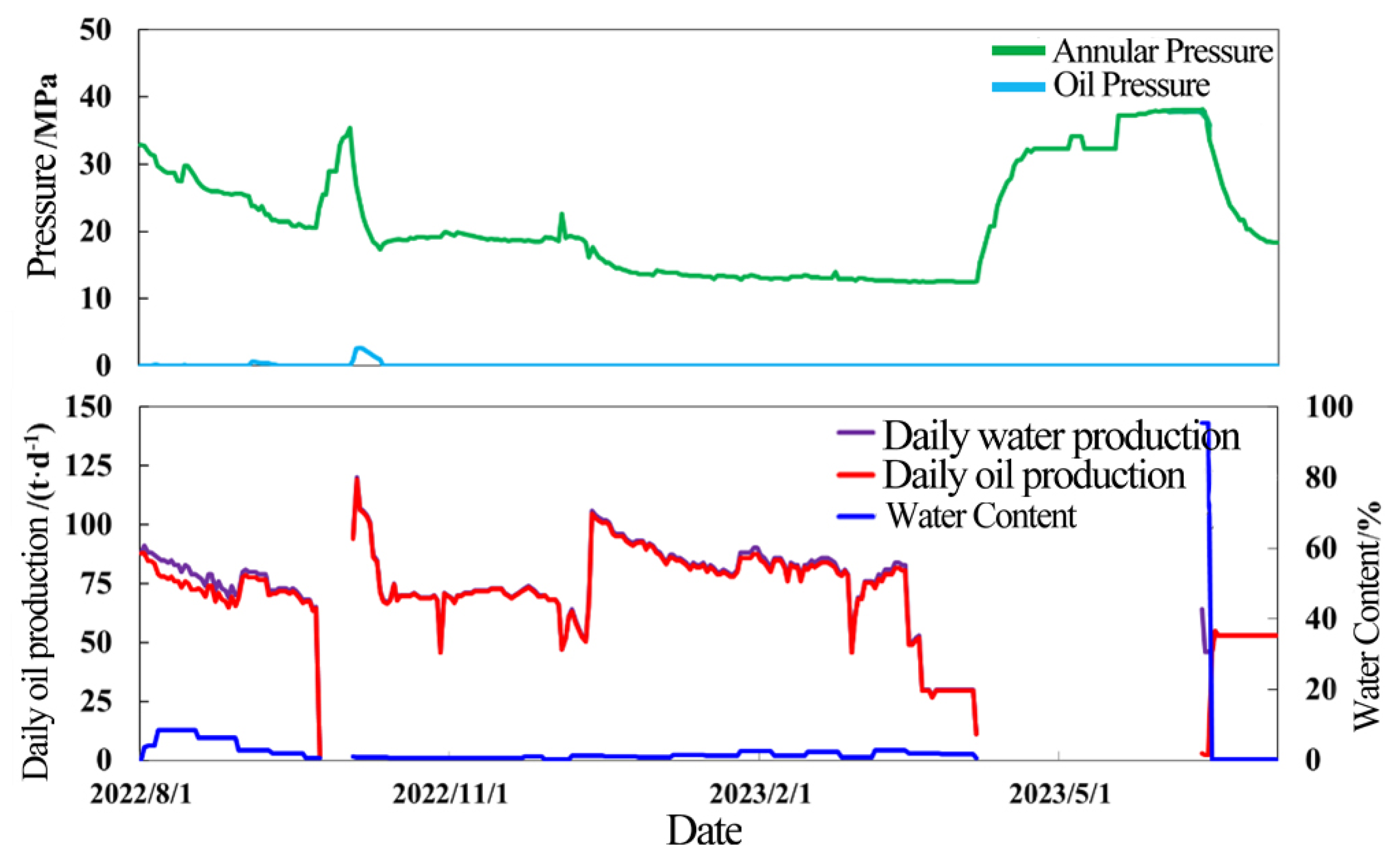
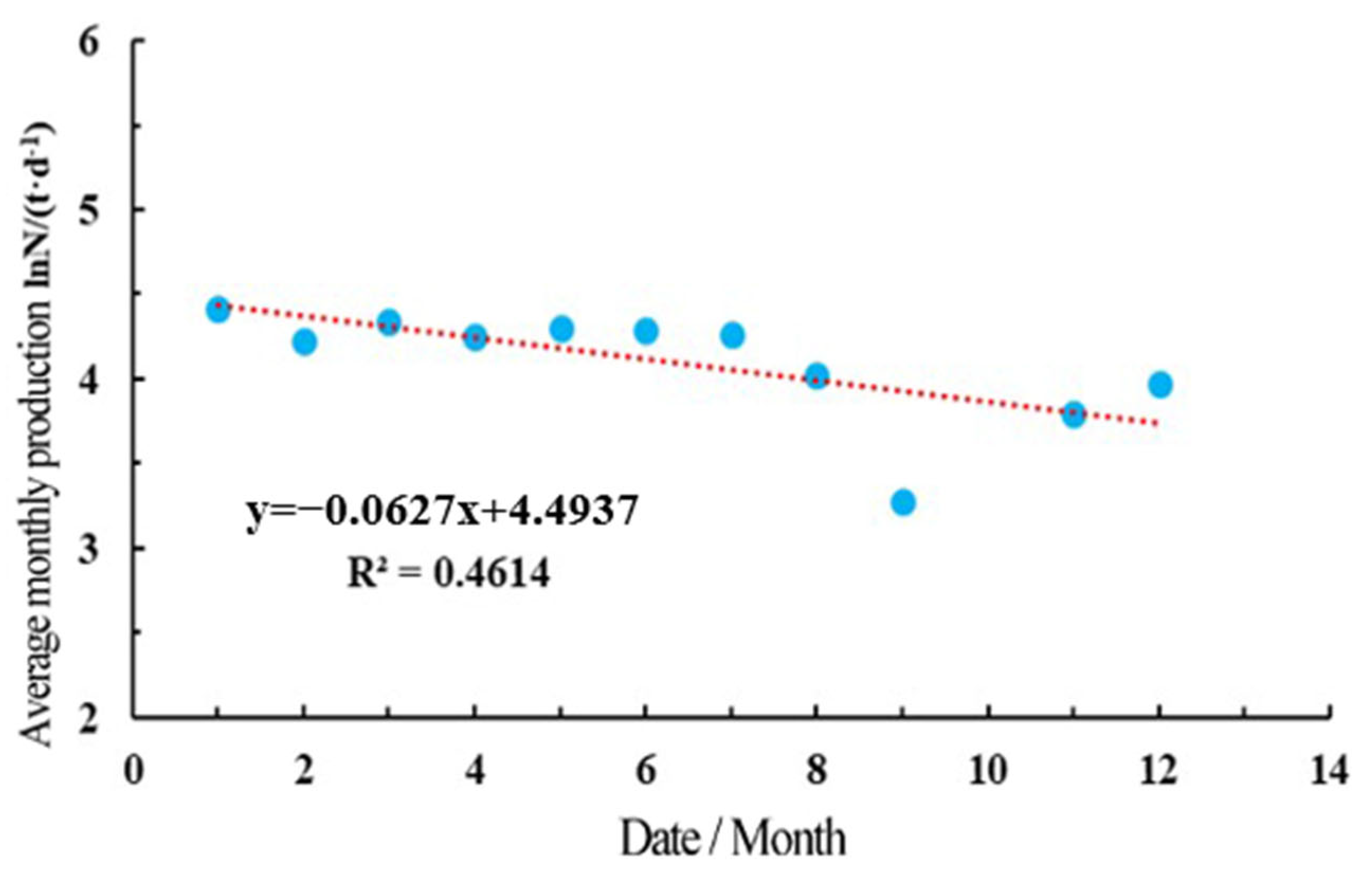
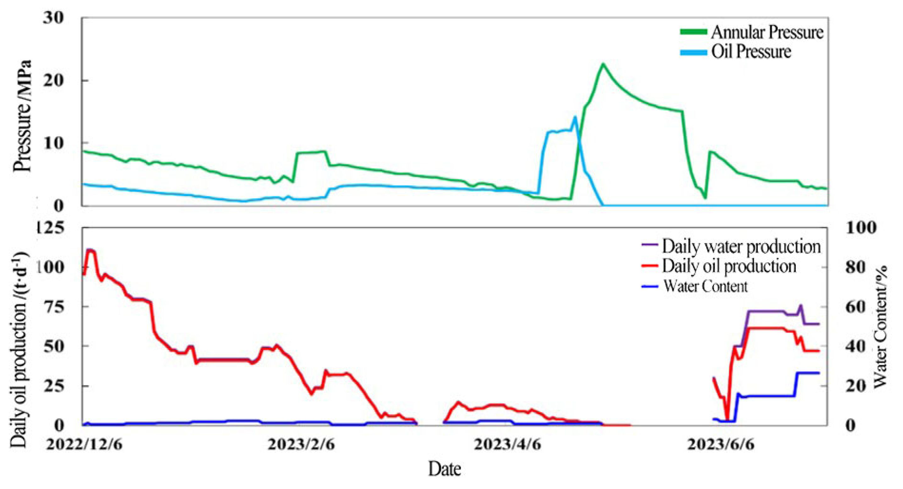
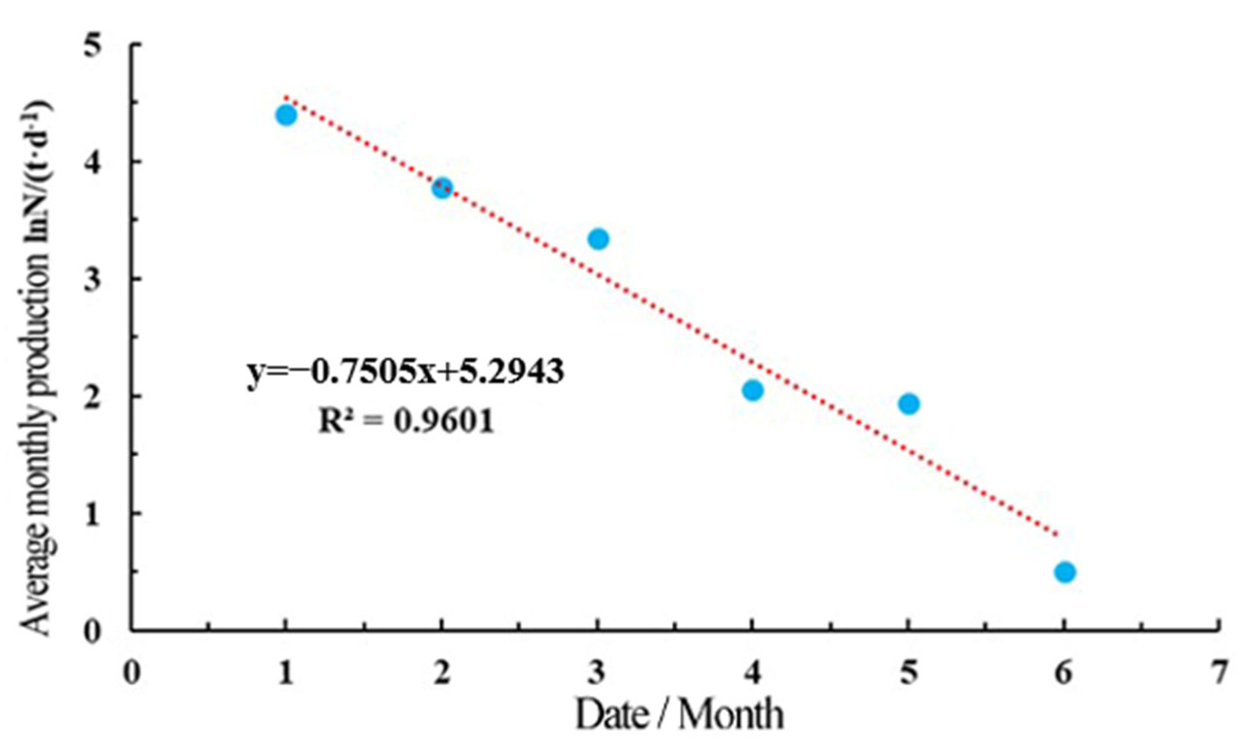
4.1. Production Characteristics of Fractured Reservoir

Fractures serve as the primary reservoir space in fractured reservoirs, offering good permeability. However, these reservoirs typically have poor overall storage capacity, characterized by insufficient natural energy and limited liquid supply capacity. In the initial stage of oil well production, water is minimal or even absent in the oil production. When water breaks through along the dominant seepage channels, the water content increases sharply, leading to violent flooding. Consequently, the overall cumulative production remains relatively low (Figure 10).

Well B504-H2 is located in the central part of the B5 well area. It was put into production on 1 August 2022. During the initial stage of production, the daily oil production was 74 t. Currently, the daily oil production is 78 t, with a water content of 2.8%. As of 31 August 2022, the cumulative oil production reached 0.2302 × 10⁴ t, and the water content increased rapidly in the later stages, exhibiting the characteristics of violent flooding.

Figure 11 shows the curve of the monthly average daily crude oil production from the B504-H2 well over time (logarithmic coordinate system). The monthly average decline rate of oil production for well B504-H2 is approximately 6.27%, indicating a rapid decline type. This well is classified as a fractured reservoir.

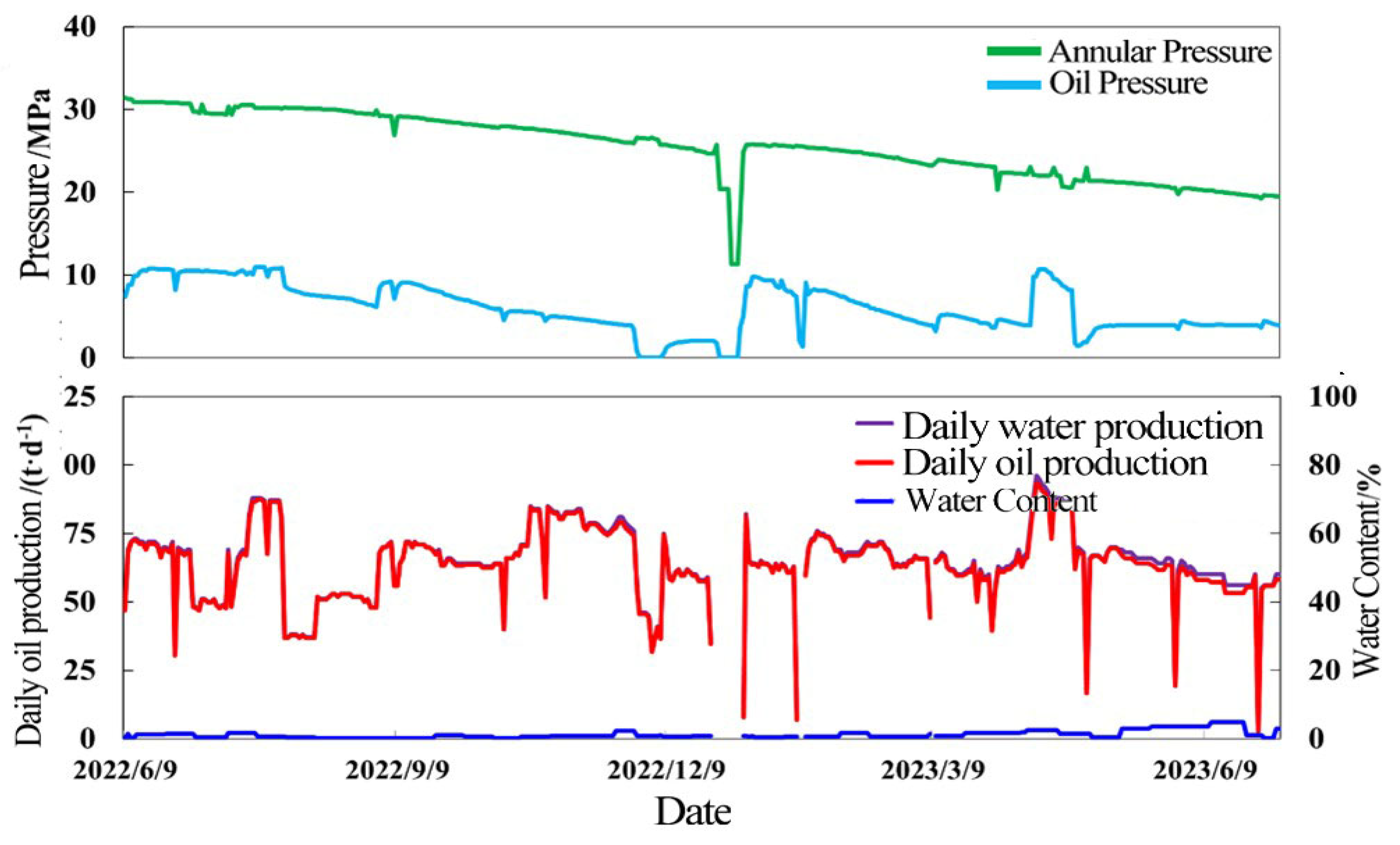
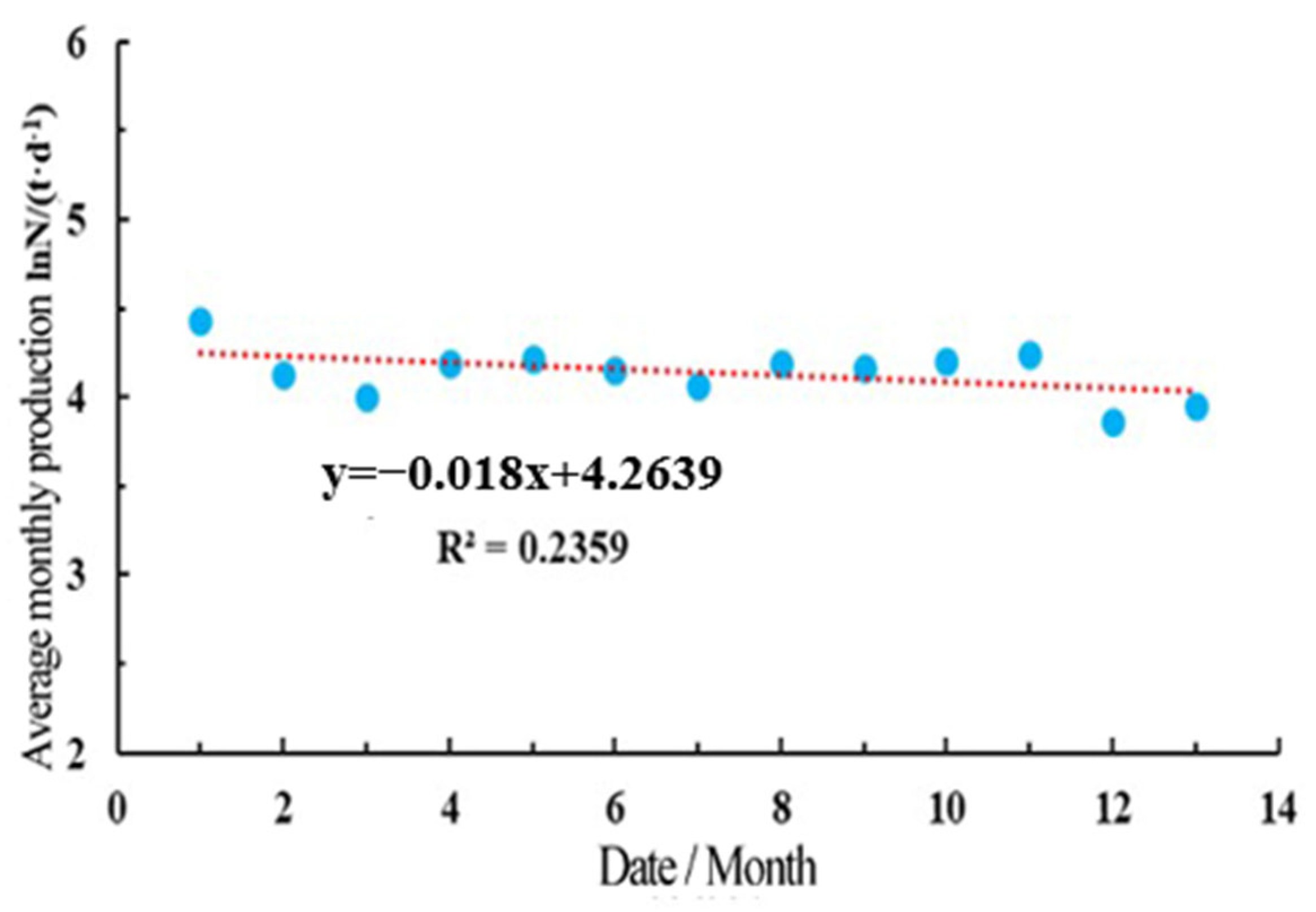
4.2. Production Characteristics of Cave Reservoir

The cave reservoir is characterized by a high initial output and a relatively high cumulative production of crude oil from a single well. During the early production stage, there is no water, and the period of water-free oil production is prolonged (Figure 12).

Well A32-H9 is located to the north of the B5 well area. It was put into production on 9 June 2022. At the beginning of production, the daily oil production was 86 t, and it has currently increased to 87 t, with a water content of 1.25%. As of 31 August 2022, the cumulative oil production reached 0.9323 × 10⁴ t, with low water content and no characteristics of violent flooding.

Figure 13 shows the curve of the monthly average daily crude oil production of the A32-H9 well over time (logarithmic coordinate system). The average monthly decline rate of oil production in well A32-H9 is approximately 1.8%, indicating a slow decline pattern. Venting and leakage occurred when drilling reached a depth of 7486.24 m. The cumulative leakage of drilling fluid was 1072.36 m³, and the intermittent venting was 12.27 m over a 9 m section. In the conventional test of the 7487.00~7634.00 m well section, a 10 mm oil nozzle was found to be equivalent to a daily oil production rate of 666 m³/d. The stable oil pressure and output indicate the presence of a large cave and sufficient natural energy. This well is a typical representative of the Karst Cave reservoir (Figure 13).

4.3. Production Characteristics of Fractured-Vuggy Reservoirs

The connectivity of fractured-vuggy reservoirs is relatively complex. Oil and gas are typically stored in dissolution pores and flow along fractures with high porosity and permeability. During the mining process, there is no violent flooding.

Well B506-H is located in the north–central part of the B5 well area. The well was put into production on 10 October 2022. At the beginning of production, the daily oil production was 10.97 t. Currently, the daily oil production has increased to 47.01 t, with a water content of 26.64%. By 4 July 2023, the cumulative oil production reached 0.6171 × 10⁴ t, with low water content and no violent flooding characteristics (Figure 14).

The production decline of the B506H well follows the exponential decline law; the fitting degree is 0.9601, and the monthly average decline rate of oil production is approximately 75.05%, indicating a high-speed decline type. Considering that no venting or leakage occurred during drilling, the well is classified as a fractured-vuggy reservoir (Figure 15).

This study identifies three distinct patterns of oil well productivity changes: slow decline, rapid decline, and high-speed decline. Wells are categorized into three connectivity groups, with the A32 well group exhibiting the highest connectivity, followed by B5 well group 1, and B5 well group 2 showing the lowest connectivity. This classification is essential for optimizing well placement and managing production strategies to maximize oil recovery.

5. Quantitative Characterization of Carbonate Reservoir Connectivity Based on Production Dynamics

5.1. Optimization of Connectivity Evaluation Index

In the process of oil and gas development, production dynamic data, pressure, and dynamic liquid level changes provide valuable insights into the hydrodynamic characteristics, pressure distribution, and energy variations within the flow unit [32]. Data on initial formation pressure, bottom-hole flow pressure, water breakthrough time, oil pressure, productivity, and dynamic liquid levels were used to qualitatively characterize reservoir connectivity. While casing pressure reflects changes in annular pressure, oil pressure serves as an indicator of the energy within the oil well. Given the high correlation between oil pressure and casing pressure, four dynamic indexes—bottom-hole flow pressure, oil pressure, productivity, and dynamic liquid level—were selected to develop a mathematical model for the quantitative evaluation of reservoir connectivity in fractured-vuggy reservoirs, enabling the precise characterization of reservoir connectivity [33].

5.2. DTW Dynamic Correlation Calculation

5.2.1. DTW Calculation Principle

The dynamic warping time (DTW) algorithm seeks the optimal mapping relationship between elements in two sequences with different lengths according to the principle of dynamic optimization and nearest distance [34]. DTW evaluates the similarity between two sequence elements by calculating the shortest regular path length (DWT distance) between elements [35,36,37,38,39].

Figure 16 shows the calculation principle of DTW dynamic correlation. Curve A and Curve B are two time series. The overall waveforms are similar, but they are not aligned on the time axis. For example, when the time point is 30, the element of sequence A is a, and the corresponding component of sequence B is b’; according to the waveform, the point corresponding to a on sequence B should be b. Traditional methods of calculating the distance between these sequences by direct comparison are not suitable. Therefore, a more effective method, such as DTW, is necessary to determine the similarity and distance between these sequences.

5.2.2. DTW Calculation Steps

Let A and B denote two time series with lengths m and n, respectively, where the distance matrix M is built. The elements in the matrix are the corresponding distance (Euclidean distance) between any two points in sequence A and B, which is called the local distance between two time points.

DTW is based on the similarity of the change characteristics between points in two time series to calculate the similarity. Therefore, it is necessary to find the corresponding mapping method between time series, which is called the regular path between time series.

$$\left\{\begin{array}{l}d(1,1)=D(a_1,b_1)\\ d(i,1)=D(a_i,b_1)+d(i-1,1)\\ d(1,j)=D(a_1,b_j)+d(1,j-1)\\ d(i,j)=D(a_i,b_j)+\min \{d(i-1,j-1),d(i-1,j),d(i,j-1)\}\end{array}\right.$$

(9)

where i = 2, 3, …, m; j = 2, 3, 4, …, n; a_i and b_j are arbitrary elements in sequence A and B, respectively; and D(a_j,b_j) is the local distance between ai and b_j.

Equation (9) is the DTW calculation methods, and the initial condition is set. The local distance accumulation is iteratively calculated from the second element of the sequence, and the minimum cumulative value d(m,n) is obtained. The minimum cumulative value is the DTW distance between sequence A and sequence B.

The similarity between time series A and B is calculated according to Equation (10):

$$dtw(A,B)={\displaystyle \frac{DTW(A,B)}{t}}$$

(10)

5.3. Quantitative Characterization of Reservoir Connectivity

The index weight analysis method is introduced to construct a calculation model for the interval connectivity of production wells. By considering the dynamic similarity between different indicators, a quantitative reservoir well connectivity model is developed to evaluate internal connectivity comprehensively. This model incorporates dynamic production data such as oil pressure, flow pressure, changes in dynamic liquid level, and productivity.

Theory of Calculation

The Analytic Hierarchy Process (AHP) is a combination of qualitative and quantitative decision-making methods, proposed by the American operations research scientist Thomas L. Saaty in the 1970s. It is suitable for multi-criteria decision-making problems, especially in the case of complex objectives, difficult to quantify data, or subjective judgment, to help decision-makers make reasonable judgments. This section introduces the index weight analysis method to establish the calculation model of inter-well connectivity of production wells. Considering the dynamic similarity between the indicators, a quantitative calculation model of reservoir well connectivity was established based on dynamic production data, such as oil pressure, flow pressure, dynamic fluid level change, and productivity, to comprehensively evaluate the well connectivity in the study area.

Figure 17 shows the structure of the analytic hierarchy process (AHP). The analysis process divides the whole problem into the highest layer, the middle layer, and the lowest layer [40]. The highest layer is the problem to be solved, that is, the target layer. The highest layer is the reservoir connectivity characterization (connectivity coefficient); the middle layer is the criterion of decision making, that is, the scheme layer, which is the similarity of four dynamic indexes such as oil pressure, flow pressure, production capacity, and dynamic liquid level change. The lowest layer is an alternative, which is not set.

A judgment (pairwise comparison) matrix was constructed. Based on the consistent matrix method proposed by Saaty et al. (1997), the relative scale is used to compare each scheme in pairs [41]. According to its importance rating, aij is the result of the comparison of the importance of elements i and j.

Table 1. Scale table of importance of matrix elements.

Factor i Compared with Factor j	Quantized Value
Equally importance	1
Slightly importance	3
Stronger importance	5
Strongly importance	7
Extremely importance	9
Two-adjacent discriminant Median	2,4,6,8

lists the nine importance ratings and quantitative values provided by Saaty.

Hierarchical single sorting and consistency tests are conducted. Considering the consistency deviation caused by random reasons, the test coefficient cr is defined as the discriminant for testing the satisfactory consistency of the discriminant matrix, as shown in Formula (11). The cr < 0.1 matrix is generally considered to pass the consistency test.

$$ci={\displaystyle \frac{{\mathsf{\lambda }}_{\max }-n}{n-1}}, ri={\displaystyle \frac{c{i}_1+c{i}_2+c{i}_3+\dots +c{i}_n}{n}}, cr=ci/ri$$

(11)

where ${\mathsf{\lambda }}_{\max }$ is the maximum eigenvalue of the discriminant matrix, n is the unique non-zero eigenvalue of the n-order consistent matrix, ci is the consistency index, and ri is the consistency evaluation index.

It is perfect consistency if ci = 0; there is satisfactory consistency if ci is close to 0; the greater ci, the stronger the inconsistency. The magnitude of ri is related to the order of the discriminant matrix; the greater the order, the greater the possibility of consistent random deviation. The correspondence between matrix order and ri is shown in

Table 2. Correspondence between the average randomness index and the order of the matrix.

Order of Matrix	1	2	3	4	5	6	7	8	9	10
ri	0	0	0.58	0.90	1.12	1.24	1.32	1.41	1.45	1.49

.

There is the calculation of weight vector D. There are three methods to calculate the weights of each indicator in hierarchical analysis: geometric method, arithmetic average method, and eigenvalue method. This weight vector D is calculated using the geometric method, as shown in Formula (12).

$$w_i={\displaystyle \frac{({\displaystyle {\prod }_{j=1}^n{a}_{ij}{)}^{\frac{1}{n}}}}{{\displaystyle {\sum }_{i=1}^n{({\displaystyle {\prod }_{j=1}^n{a}_{ij}})}^{\frac{1}{n}}}}},i=1,2,3\dots n$$

(12)

The weights corresponding to each indicator are calculated based on the constructed discriminant matrix, as shown in

Table 3. Dynamic indicator weight calculation table.

Index	Oil Pressure	Flow Pressure	Production Capacity	Dynamic Liquid Level	ci	ri	cr	Weights wi
Oil pressure	1	2	1/2	3	0.00484	0.90	0.00542	0.2717
Flow pressure	1/2	1	1/3	2				0.1569
Production capacity	2	3	1	5				0.4832
Dynamic liquid level	1/3	1/2	1/5	1				0.0882

.

It can be seen from Table 3 that the corresponding weights of oil pressure, flow pressure, production capacity, and dynamic liquid level are 0.2717, 0.1569, 0.4832, and 0.0882, respectively. The calculation results are in line with the production law of the mine, and the test coefficient cr < 0.1, which satisfies the consistency test, and can be carried out in the next step of the evaluation of the connectivity of the oil wells.

(2) Calculation Model

Four production dynamic indicators—oil pressure, flow pressure, oil production capacity, and dynamic liquid level change—are selected as the key factors to characterize the connectivity of reservoir wells. Given the limitations of using a single index for description, a comprehensive evaluation model of reservoir connectivity was developed to quantitatively assess the connectivity of fractured-vuggy reservoirs. This model incorporates dynamic production data, including oil pressure, flow pressure, oil production capacity, and changes in dynamic liquid level, to provide a more holistic view of reservoir connectivity throughout the production process.

Through oil pressure, flow pressure, initial formation pressure, and other factors, the well group division of the B5 block in the study area was carried out, and the overall connectivity of each well group was qualitatively analyzed. Oil pressure was used to determine the threshold for inter-well connectivity discrimination in the seam-hole unit.

The group distance is calculated by the Sturger empirical formula, as shown in Formula (13):

$$f=1+3.322\lg N$$

(13)

In the formula, f is the group distance of the oil pressure curve, and N is the number of DTW values of all oil pressure curves inside the fractured-vuggy unit.

If the minimum or maximum value of the DTW value are directly used to set the connectivity threshold, it may be affected by outliers. The two intervals with the largest distribution of oil pressure DTW data are selected, and the average value of each DTW value in the interval is calculated as its discriminant threshold. It can effectively reduce the interference of outliers and make the discrimination result more stable.

A mathematical model for inter-well connectivity evaluation is established based on single-indicator connectivity analysis, as shown in Formula (14).

$$I_c={\displaystyle \sum _{j=1}^4[(2-\frac{y_{ij}}{\underset{1<i<n}{\max }(y_{ij})-\underset{1<i<n}{\min }(y_{ij})})\times W_j]}$$

(14)

In this formula, I_c is the reservoir connectivity coefficient, dimensionless; y_ij is the value of an evaluation index for reservoir wells; maxy_ij and miny_ij are the maximum and minimum values of an evaluation index, respectively; j is the number of evaluation indexes, here, take j = 4; and W_j is the index weighting coefficient.

5.4. Reservoir Connectivity Evaluation in the Study Area

In the study area, the B5 well zone is located along the F_I17 fault zone, representing a typical fault-controlled fractured-vuggy reservoir [42,43]. Building on the qualitative analysis of reservoir connectivity, a similarity analysis of dynamic characteristics between wells was conducted to achieve the quantitative characterization of inter-well connectivity.

(1) Production dynamic similarity calculation

The production dynamic curve can be regarded as a time series of a certain length. The similarity between two time series can be discriminated by calculating their DTW values; the smaller the DTW value, the higher the similarity, indicating a better degree of connectivity between the two wells. Conversely, the larger the DTW value, the worse the connectivity between the wells. Based on the four dynamic indicators of bottom-hole flow pressure, production, oil pressure, and dynamic liquid level, the inter-well similarity analysis is conducted. To visualize the similarity of well development indexes, the dynamic characteristic curves between two wells in the A32 well group are plotted, as shown in Figure 18.

Firstly, the single-index connectivity identification is carried out in the B5 well area, and the dynamic correlation of the curve is calculated according to Equation (2). Due to the complexity of the sequence and the huge amount of calculation, MATLAB R2023b software was used to iteratively accumulate the curve DTW values. The dynamic similarity thresholds for the well flow pressure, oil pressure, production capacity, and dynamic liquid level curves were calculated as 2.150, 1.553, 17.135, and 189.480, respectively. The dynamic similarity of the well group is summarized in

Table 4. Similarity of dynamic characteristics of similar wells in the A32 well group.

Connecting Well Number	Dynamic Feature Similarity
	Wellhole Flowing Pressure	Oil Pressure	Production Capacity	Dynamic Liquid Level
A32-H5, A32-H7	0.419	0.070	3.388	60.601
A32-H1, A32-H9	0.827	0.138	7.571	110.171
A32-H1, A32-H5	1.181	0.197	10.940	119.244
A32-H1, A32-H7	0.945	0.157	8.533	140.959
A32-H9, A32-H5	1.614	0.269	9.778	142.933
A32-H9, A32-H7	1.418	0.236	9.843	122.357

,

Table 5. Similarity of dynamic characteristics of similar wells in B5 well group 1.

Connecting Well Number	Dynamic Feature Similarity
	Wellhole Flowing Pressure	Oil Pressure	Production Capacity	Dynamic Liquid Level
BH8, BH9	0.739	-	4.561	128.880
B501H, BH2	1.294	0.088	-	141.182
BH2, B5	1.172	-	6.345	-
BH6, B5	0.910	-	-	93.955
BH6, BH9	-	0.179	-	-
B5, BH8	-	0.673	-	-
BH2, BH9	-	-	3.586	-
B501H, BH8	-	-	6.982	-

and

Table 6. Similarity of dynamic characteristics of similar wells in B5 well group 2.

Dynamic Similarity Index	Connecting Well Number	Dynamic Feature Similarity
Wellhole flowing pressure	B501-H1, BH4	0.889
Oil pressure	BH4, B501-H1	0.937
	B504H, B501-H1	0.608
Production capacity	B501-H1, BH4	5.824
Dynamic liquid level	B501-H1, BH4	103.464

.

(2) Inter-well connectivity coefficient

Based on the calculation results of the similarity of dynamic features between wells and the mathematical model of inter-well connectivity evaluation, the inter-well connectivity coefficient is calculated, as shown in

Table 7. Inter-well connectivity coefficient of wells in five well area.

Connecting Well Number	Connectivity Coefficient Ic	Connecting Well Number	Connectivity Coefficient Ic
A32-H5, A32-H7	1.746	B501H, BH2	1.249
A32-H1, A32-H9	1.470	BH2, B5	1.317
A32-H1, A32-H5	1.267	BH6, B5	0.942
A32-H1, A32-H7	1.388	BH6, BH9	1.090
A32-H9, A32-H5	1.226	BH2, BH9	1.310
A32-H9, A32-H7	1.271	B501H, BH8	1.214
BH8, BH9	1.565	B501-H1, BH4	1.380

.

Table 7 shows the connectivity coefficients between the connected oil wells in the ManS 5 well area. A higher connectivity coefficient indicates better connectivity between two producing wells, meaning better reservoir connectivity. Six sets of connectivity coefficients of the A32 well group are greater than those of the B5 well group, which indicates that the reservoir connectivity is the best in the A32 well group, and the conclusions are in line with the results of the qualitative analysis of the connectivity, as mentioned before.

It can be seen from Table 7 that the greater the connectivity coefficient, the better the connectivity between the two production wells, that is, the better the reservoir connectivity. The six groups of connectivity coefficients of the A32 well group are greater than those of the B5 well group, indicating that the reservoir connectivity of the A32 well group is the best. The conclusion is consistent with the qualitative analysis results of the connectivity above.

All four wells in the A32 well group are multi-connected, and the schematic diagrams of the well connections in the study area are drawn, as shown in Figure 19. From Figure 19, it can be seen that the reservoir connectivity of B5 well group 2 is different from that of the A32 well group and B5 well group 1, in which B504-H2 has poor connectivity with other wells, reflecting the poor reservoir connectivity around the well.

6. Conclusions

Based on dynamic production data, the reservoir connectivity of the target layers in the study area is evaluated, using the preferred evaluation indexes. Inter-well connectivity is analyzed from multiple aspects, and a multi-index mathematical model is developed for quantitative characterization. The following conclusions and insights are drawn.

(1) Based on the characteristics of declining production, the capacity changes in production wells are classified into three distinct patterns: gradual decline, rapid decline, and steep decline. In accordance with the increasing water cut trend, changes in water content are categorized into five types: gradual increase, sharp rise, storm flooding, stepwise increase, and fluctuation.

(2) The model uses the heat diffusion equation and multi-source potential field method to calculate connectivity probability and intensity in fractured-vuggy reservoirs. The results, validated through an integrated multi-information approach, classify connectivity into four levels. High connectivity is observed near BH8 and BH9 wells, while the BH6 well area shows weak connectivity, with S_total < 0.1.

(3) Based on the characteristics of water breakthrough and the trend of formation pressure variation, the production wells in the study area are classified into three interconnected well groups. The connectivity of each well group is qualitatively analyzed through the observed changes in bottom-hole flow pressure, oil pressure, productivity, and dynamic liquid level. The analysis reveals that the A32 well group exhibits the highest connectivity, followed by the B5 well group 1, and the B5 well group 2 showing the weakest connectivity.

(4) The DTW algorithm and index weight analysis method are applied to comprehensively evaluate dynamic production indices, including bottom-hole flow pressure, oil pressure, productivity, and dynamic liquid level. A mathematical model is developed to quantitatively characterize the macro-level reservoir connectivity. By calculating the similarity and connectivity coefficients of these dynamic indices within the interconnected well groups, a quantitative assessment of inter-well connectivity is achieved.

This study’s proposed connectivity analysis significantly enhances the understanding of fractured-vuggy marine carbonate reservoirs by providing a more comprehensive and precise approach than traditional methods. It integrates dynamic production data with advanced mathematical models, such as the heat diffusion equation, dynamic warping time (DTW) algorithm, and analytic hierarchy process (AHP), offering a detailed characterization of reservoir connectivity. This represents a significant improvement over traditional methods, which often rely on qualitative assessments or simpler quantitative models that may not fully capture the complexity of reservoir connectivity.

This study also presents significant practical implications by providing a comprehensive and quantitative assessment of reservoir connectivity in fractured-vuggy marine carbonate reservoirs. Future research could explore the integration of machine learning techniques to further refine connectivity predictions and enhance the accuracy of reservoir characterization. Additionally, advanced methods such as deep learning and multi-physics simulations could be employed to better understand the complex interactions within these reservoirs and to develop more efficient oil recovery strategies.

The research results hold significant potential for application beyond the Tarim Basin to other similar geological structures. The methodologies used, such as the heat diffusion equation, DTW algorithm, and AHP model, can be adapted to other fractured-vuggy carbonate reservoirs worldwide. However, the study has limitations, including the complexity of the geological environment, dependence on potentially flawed production data, DTW’s data handling limitations, and the study’s specific focus. And the study uses the heat diffusion equation to calculate reservoir connectivity; this method is based on probabilistic statistics, which can have some uncertainties, and is not applicable to different future development stages. Despite these, the methods offer valuable insights but require careful consideration of geological complexity, data quality, and analytical limitations. Future work could focus on better data acquisition, advanced modeling, and more case studies to address these challenges.

References

1. Jiabei, X.; Dengfa, H. Distribution characteristics and controlling factors of global giant carbonate stratigraphic-lithologic oil and gas fields. Lithol. Reserv. 2022, 34, 187–200. [Google Scholar]
2. Huaxin, C.; Zhihong, K.; Zhijiang, K. Stratified Structure and Formation Mechanism of Paleokarst Cave in Carbonate Reservoir of Tahe Oilfield. Geoscience 2022, 36, 695–708. [Google Scholar]
3. Zhijiang, K.; Yang, L.; Bingyu, J. Key technologies for EOR in fractured-vuggy carbonate reservoirs. Oil Gas Geol. 2020, 41, 434–441. [Google Scholar]
4. Liaoyuan, H. Study on the Connectivity of Fracture-Cavity Bodies and Remaining Oil Distribution in Yingshan Formation of Zhonggu 8 Well Block. China Univ. Pet. 2021. [Google Scholar]
5. Elmo, D.; Rogers, S.; Stead, D.; Eberhardt, E. Discrete Fracture Network approach to characterise rock mass fragmentation and implications for geomechanical upscaling. Min. Technol. 2014, 123, 149–161. [Google Scholar] [CrossRef]
6. Medici, G.; Ling, F.; Shang, J. Review of discrete fracture network characterization for geothermal energy extraction. Front. Earth Sci. 2023, 11, 1328397. [Google Scholar] [CrossRef]
7. Dumitrache, L.; Roy, A.; Bird, A.; Goktas, B.; Sorgi, C.; Stanley, R.; De Gennaro, V.; Eswein, E.; Abbott, J. A Multidisciplinary Approach to Production Optimization through Hydraulic Fracturing Stimulation and Geomechanical Modelling in Clair Field. In Proceedings of the International Petroleum Technology Conference, Riyadh, Saudi Arabia, 21–23 February 2022. [Google Scholar]
8. Lingling, Y.; Quanwen, L.; Xuefen, L. Research on 3D geological modeling of fractured-vuggy carbonate reservoirs. In Proceedings of the 7th International Conference on Advances in Energy Resources and Environment Engineering (ICAESEE 2021), Guangzhou, China, 19–21 November 2021. [Google Scholar]
9. Huichao, Y.; Gaizhuo, Z.; Qiang, W.; Fangpeng, C.; Bicheng, Y.; Shangxian, Y.; Soltanian, M.R.; Thanh, H.V.; Zhenxue, D. Unraveling Overlying Rock Fracturing Evolvement for Mining Water Inflow Channel Prediction: A Spatiotemporal Analysis Using ConvLSTM Image Reconstruction. IEEE Trans. Geosci. Remote Sens. 2024. [Google Scholar] [CrossRef]
10. Ren, M.; Wang, Z.; Jiang, Q.; Hu, G.; Fan, T.; Fan, H. The carbonate reservoir characteristics and pore genesis in the Middle Permian Maokou Formation, Southern Sichuan Basin. J. Northeast. Pet. Univ. 2021, 45, 32–43. [Google Scholar]
11. Zhang, J.; Yang, M.; Xie, R.; Wang, M.; Wang, H.; Luo, Z. Probability-constrained identification of Ordovician small-scale fractured-vuggy reservoirs in Blocks 4–6. Oil Gas Geol. 2022, 43, 219–228. [Google Scholar]
12. Sun, L.; Wang, X.; Jin, X.; Li, J.; Wu, S. Three-dimensional characterization and quantitative connectivity analysis of micro/nanopore space. Pet. Explor. Dev. 2016, 43, 490–498. [Google Scholar] [CrossRef]
13. Tian, G.; Qi, C.; Yuchan, Z.; Lv, J. Quantitative characterization of connectivity of fractured vuggy carbonate reservoirs. Petrochem. Ind. Technol. 2021, 28, 116–117. [Google Scholar]
14. Zhihong, K.; Lin, C.; Xinbian, L.; Yang, M. Fluid dynamic connectivity of karst carbonate reservoir with fracture & cave system in Tahe Oilfield. Earth Sci. Front. 2012, 19, 110–120. [Google Scholar]
15. Zhao, H.; Li, B.; Zhou, Y.; Zhang, Q.; Liu, H.; Wang, W.; Wang, X. A connectivity prediction model for fault-karst reservoirs based on high-speed non-Darcy flow. Acta Pet. Sin. 2022, 43, 1026–1034. [Google Scholar]
16. Fanjing, K. Connectivity of Ordovician fractured vuggy reservoirs in Zhonggu 8 area, Tazhong. In Proceedings of the International Field Exploration and Development Conference, Qingdao, China, 20–22 October 2021; Volume I, pp. 48–49. [Google Scholar]
17. Zhonghua, C.; Shouyu, X.; Changmin, X. Study on the Connectivity of Ordovician Fault-karst Reservoir in Yueman Block Halahatang Oilfield. J. Gansu Sci. 2023, 35, 22–30. [Google Scholar]
18. Zhesi, C.; Qiyu, C.; Jian, L.; Xiaogang, M.; Gang, L. Characterizing subsurface structures from hard and soft data with multiple-condition fusion neural network. Water Resour. Res. 2024, 60, e2024WR038170. [Google Scholar]
19. Li, J.; Kong, X.C.; Song, M.S.; Wang, Y.; Wang, H.; Liu, X.L. Study on the influence of reservoir rock micro-pore structure on rock mechanical properties and crack propagation. Rock Soil Mech. 2019, 40, 4149–4156. [Google Scholar]
20. Gou, Q.; Xu, S.; Hao, F.; Yang, F.; Wang, Y.; Lu, Y.; Gao, M. Study on characterization of micro-fracture of shale based on micro-CT. Acta Geol. Sin. 2019, 93, 2372–2382. [Google Scholar]
21. Dinh, A.; Tiab, D. Inferring Interwell Connectivity from Well Bottomhole-Pressure Fluctuations in Waterfloods. SPE Reserv. Eval. Eng. 2008, 11, 874–881. [Google Scholar] [CrossRef]
22. Jinzi, L. Potential for Evaluation of Interwell Connectivity under the Effect of Intraformational Bed in Reservoirs Utilizing Machine Learning Methods. Geofluids 2020, 2020, 1651549. [Google Scholar]
23. Zhang, X.; Huang, Z.; Lei, Q.; Yao, J.; Gong, L.; Sun, S.; Li, Y. Connectivity, permeability, and flow channelization in fractured karst reservoirs: A numerical investigation based on a two-dimensional discrete fracture-cave network model. Adv. Water Resour. 2022, 161, 104142. [Google Scholar] [CrossRef]
24. Wang, D.; Li, Y.; Hu, Y.; Li, B.; Deng, X.; Liu, Z. Integrated dynamic evaluation of depletion-drive performance in naturally fractured-vuggy carbonate reservoirs using DPSO–FCM clustering. Fuel 2016, 181, 996–1010. [Google Scholar] [CrossRef]
25. Patidar, A.K.; Joshi, D.; Dristant, U.; Choudhury, T. A review of tracer testing techniques in porous media specially attributed to the oil and gas industry. J. Pet. Explor. Prod. Technol. 2022, 12, 3339–3356. [Google Scholar] [CrossRef]
26. Dong, X.; Liping, C.; Xiaofeng, X.; Gui, T.; Yongbo, H.; Boyun, G.; Mingjie, L.; Chenxu, Y.; Gao, L. Coupling model of wellbore heat transfer and cuttings bed height during horizontal well drilling. Phys. Fluids 2024, 36, 097163. [Google Scholar]
27. Zhenxue, D.; Wolfsberg, A.; Lu, Z.; Ritzi, R., Jr. Representing aquifer architecture in macrodispersivity models with an analytical solution of the transition probability matrix. Geophys. Res. Lett. 2007, 34, L20406. [Google Scholar] [CrossRef]
28. Ning, C.; Sun, L.; Hu, S.; Xu, H.; Pan, W.; Li, Y.; Zhao, K. Karst types and characteristics of the Ordovician fracture-cavity type carbonate reservoirs in Halahatang oilfield, Tarim Basin. Acta Pet. Sin. 2021, 42, 15–32. [Google Scholar]
29. Du, X.; Dong, S.; Zeng, L.; He, J.; Sun, F. Study of automatic extraction porosity using cast thin sections for carbonates. Geol. Rev. 2021, 67, 1910–1921. [Google Scholar]
30. Zhang, S.; Wang, X.; Ren, X.; Xiong, Y.; Lin, W. Identification Method for Carbonate Rock Supergene Karst Characteristics. Well Logging Technol. 2022, 46, 274–282. [Google Scholar]
31. Xuan, C.; Wanghan, L.; Dian, B.; Zhang, L.; Chen, L.; Yang, M.; Jia, Y. Filling Ages Identifications and its reservoirs are significant for filling materials of Ordovician Palaeo-karst Caves in Tahe Oilfield. Earth Sci. Front. 2023, 30, 65–75. [Google Scholar]
32. Wu, M.; Chai, X.; Zhou, B.; Li, H.; Yan, N.; Peng, P. Connectivity Characterization of Fractured-Vuggy Carbonate Reservoirs and Application. Xinjiang Pet. Geol. 2022, 43, 188–193. [Google Scholar]
33. Liu, Y.; Rong, Y.S.; Yang, M. Detailed classification and evaluation of reserves in fracture-cavity units for carbonate fracture-cavity reservoirs. Pet. Geol. Exp. 2018, 40, 431–438. [Google Scholar]
34. Müller, M. Information Retrieval for Music and Motion; Springer: Berlin/Heidelberg, Germany, 2007; pp. 69–84. [Google Scholar]
35. Li, H. Time works well: Dynamic time warping based on time weighting for time series data mining. Inf. Sci. 2021, 547, 592–608. [Google Scholar] [CrossRef]
36. Hong, J.Y.; Park, S.H.; Baek, J.G. SSDTW: Shape segment dynamic time warping. Expert Syst. Appl. 2020, 150, 113291. [Google Scholar] [CrossRef]
37. Hernandez-Mejia, J.L.; Pisel, J.; Jo, H.; Pyrcz, M.J. Dynamic time warping for well injection and production history connectivity characterization. Comput. Geosci. 2023, 27, 159–178. [Google Scholar] [CrossRef]
38. Meng, F.; Fan, X.; Chen, S.Y.; Ye, Y.Y.; Jiang, H.; Pan, W.; Wu, F.; Zhang, H.; Chen, Y.; Semnani, A. Automatic Well-Log Depth Shift with Multilevel Wavelet Decomposition Network and Dynamic Time Warping. Geoenergy Sci. Eng. 2024, 246, 213583. [Google Scholar] [CrossRef]
39. Dürrenmatt, D.J.; Del Giudice, D.; Rieckermann, J. Dynamic time warping improves sewer flow monitoring. Water Res. 2013, 47, 3803–3816. [Google Scholar] [CrossRef] [PubMed]
40. Liu, X.; Zhang, W.; Qu, Z.; Guo, T.; Sun, Y.; Rabiei, M.; Cao, Q. Feasibility evaluation of hydraulic fracturing in hydrate-bearing sediments based on analytic hierarchy process-entropy method (AHP-EM). J. Nat. Gas Sci. Eng. 2020, 81, 103434. [Google Scholar] [CrossRef]
41. Saaty, T.L. A scaling method for priorities in hierarchical structures. J. Math. Psychol. 1977, 15, 234–281. [Google Scholar] [CrossRef]
42. Li, Z.; Li, H.; Liu, J.; Deng, G.; Gu, H.; Yan, Z. 3D seismic intelligent prediction of fault-controlled fractured-vuggy reservoirs in carbonate reservoirs based on a deep learning method. J. Geophys. Eng. 2024, 21, 345–358. [Google Scholar] [CrossRef]
43. Wang, J.; Qi, X.; Liu, H.; Yang, M.; Li, X.; Liu, H.; Zhang, T. Mechanisms of remaining oil formation by water flooding and enhanced oil recovery by reversing water injection in fractured-vuggy reservoirs. Pet. Explor. Dev. 2022, 49, 1110–1125. [Google Scholar] [CrossRef]
Figure 1. Structural location of the study area.
Jmse 13 00435 g001
Figure 2. Log response characteristics of karst cave reservoir space in the study area.
Jmse 13 00435 g002
Figure 3. Well logging response characteristics of dissolution cavity type reservoir space.
Jmse 13 00435 g003
Figure 4. Development characteristics of reservoir core dissolution cavity in the study area (according to the internal data of PetroChina Tarim Oilfield, 2023): (a) Well FA (7410.00 m); (b) Well FB (7411.00 m).
Jmse 13 00435 g004
Figure 5. Development characteristics of reservoir core fractures in the study area (according to the internal data of PetroChina Tarim Oilfield, 2023).
Jmse 13 00435 g005
Figure 6. Typical core slices of Yijianfang Formation in the study area (according to PetroChina Tarim oilfield internal data perfect, 2023): (a) Well FB (7607.81 m); (b) Well FB (7610.51 m); (c) Well FA (7404.25 m); (d) Well FA (7371.07 m); (e) Well FB-3 (8228.90 m); (f) Well FB-3 (8230.30 m).
Jmse 13 00435 g006
Figure 7. Diagram of inter-well reservoir connectivity modes: (a) rack connectivity; (b) karst connectivity; (c) fractured-vuggy connectivity.
Jmse 13 00435 g007
Figure 8. Three-dimensional sculpting of the integration of different attributes and connectivity intensities within the reservoir.
Jmse 13 00435 g008
Figure 9. Contour map of the connectivity probability distribution based on the fusion of different attributes in key well areas of the study zone.
Jmse 13 00435 g009
Figure 10. Production dynamic performance curve of well B504−H2.
Jmse 13 00435 g010
Figure 11. B504−H2 well production decline fitting curve.
Jmse 13 00435 g011
Figure 12. Production dynamic performance curve of well A32−H9.
Jmse 13 00435 g012
Figure 13. A32-H9 well production decline fitting curve.
Jmse 13 00435 g013
Figure 14. Production dynamic performance curve of well B506H.
Jmse 13 00435 g014
Figure 15. B506-H2 well production decline fitting curve.
Jmse 13 00435 g015
Figure 16. DTW dynamic correlation calculation principle: (a) DTW mapping relationship between one-dimensional; (b) DTW optimal path selection diagram time series elements.
Jmse 13 00435 g016
Figure 17. Analytic hierarchy process structure diagram.
Jmse 13 00435 g017
Figure 18. Dynamic characteristic curve between two wells of well group A32.
Jmse 13 00435 g018aJmse 13 00435 g018b
Figure 19. Production well connection diagram of Bhen 5 well area: (a) A32 well group; (b) B5 well group 1; (c) B5 well group 2.
Jmse 13 00435 g019