A Symbol Conditional Entropy-Based Method for Incipient Cavitation Prediction in Hydraulic Turbines

Abstract

The accurate prediction of incipient cavitation is of great significance for ensuring the stable operation of hydraulic turbines. Hydroacoustic signals contain essential information about the turbine’s operating state. Considering that traditional entropy methods are easily affected by environmental noise when the state pattern is chaotic, leading to the extracted cavitation features not being obvious, a Symbol Conditional Entropy (SCE) feature extraction method is proposed to classify the original variables according to different state patterns. The uncertainty is reduced, and the ability to extract fault information is improved, so more effective cavitation features can be extracted to describe the evolving trend of cavitation. The extracted cavitation features are used as indicators to predict incipient cavitation. In order to avoid missing critical information in the prediction process, an interval mean (IM) algorithm is proposed to determine the initial prediction point. The effectiveness of the proposed method is validated with hydroacoustic signals collected at the Harbin Institute of Large Electric Machinery. The root mean square error (RMSE), mean absolute error (MAE), and mean absolute percentage error (MAPE) of incipient cavitation prediction results decreased to 0.0018, 0.0015, and 1.59%, respectively. The RMSE, MAE, and MAPE of the proposed SCE decreased by 84.62%, 85.29%, and 87% compared with the Permutation Entropy (PE) method. The comparison results with different prediction algorithms show that the proposed SCE has excellent trend prediction performance and high precision.

1. Introduction

Hydropower is a green and low-carbon renewable energy source that can provide competitive and flexible power [1]. The hydraulic turbine is a crucial component in any hydropower plant [2]. Once the turbine operates abnormally or encounters accidents, it will affect the stability and economic benefits of the power plant [3], and may even lead to accidents in the power station [4,5]. When the turbine operates at the off-design operating point, the gradual decrease in water pressure leads to instability and cavitation phenomena. Cavitation erosion is the most common origin of destruction of hydraulic mechanical systems [6,7,8]. Long-term operation in the cavitation state will lead to corrosion of the metal surface of the turbine [9]. Moreover, the increase of cavitation degree will not only cause damage to the mechanical equipment, but also reduce the power generation efficiency [10,11]. Predicting the cavitation evolution trend is helpful to adjust the mechanical parameters in time, reduce the cavitation degree and extend the machine’s lifespan. Accordingly, predicting the cavitation is highly relevant to preventing the increase in the cavitation degree [12].

Computational Fluid Dynamics (CFD) and other numerical simulation methods are widely employed to simulate the cavitation phenomenon in hydraulic turbines [13,14]. These simulations can be employed to predict the location, intensity, and potential consequences of the cavitation, thus assisting engineers in taking precautionary measures [15]. Nevertheless, due to the uncertainties in the turbulence model, the high computational cost, and the challenges with high-precision turbulence simulation, it is tedious to obtain a reliable prediction of the cavitation with only simulation results. Therefore, an increasing amount of attention has been paid to experimental methods for studying cavitation through testing physical models in laboratories [16,17]. Hydroacoustic signals contain essential information about the turbine’s operating state [18]. By analyzing the hydroacoustic signals generated during mechanical operation, different cavitation states can be identified [19]. Kang et al. [20] studied the characteristics of incipient cavitation by analyzing hydroacoustic signals. Although experimental methods have been successful in identifying different cavitation states, there are few relevant studies on the prediction of incipient cavitation trends in hydraulic turbines [21,22]. The extraction of the cavitation feature is the key point for incipient cavitation prediction. This feature is helpful for characterizing the evolving trend of cavitation and improves the prediction accuracy. An effective strategy is to predict the incipient cavitation by predicting the evolution trend of the indicator feature that can quantitatively characterize the turbine cavitation degree. Extracting the fault feature that can quantitatively characterize the trend of turbine cavitation is an essential step for accurate cavitation prediction. Entropy is a powerful and effective tool for characterizing nonlinear changes in data [23]. It is widely used in fault diagnosis [24]. The higher the data irregularity, the higher the entropy. The most widely used methods include Permutation Entropy (PE) and Fuzzy Entropy (FE) [25,26]. Li et al. [27] effectively extracted features of ship-radiated noise by computing the PE of the intrinsic mode functions. Modular multilevel converter high-voltage direct current transmission line faults are identified based on the Permutation Entropy algorithm [28]. PE is sensitive to the nonlinearity and non-stationarity of signals, allowing for the measurement of uncertainty in time series, and it has high computational efficiency. However, it is relatively sensitive to noise, and direct application for extracting cavitation indicator features is affected by a large amount of random noise, making it difficult to extract critical cavitation information. B. Saravanan et al. [29] reduced data dimensionality by using FE for feature selection. Hou et al. [30] proposed a new gearbox fault diagnosis method based on Fuzzy Entropy, which can effectively extract the nonlinear fault features of the gearbox. Zhou et al. [31] proposed a hierarchical multiscale fluctuation-based symbolic FE method with obvious advantages in nonlinear feature extraction. Although FE exhibits relatively strong robustness to noise, it is still affected by the weak signal of incipient cavitation-radiated noise, making it difficult to extract indicator features. Li et al. [32] proposed Symbol Dynamic Entropy (SDE) to fit the dynamic characteristics of vibration signals. SDE can effectively remove background noise using a symbolization process and retain fault information using the probability of state patterns and state transitions. Yang et al. [33] developed enhanced hierarchical symbolic dynamic entropy (EHSDE) to extract a more useful feature representation. SDE has been shown to perform better in analyzing vibration signals using amplitude and frequency information. SDE has obvious advantages, such as higher computational efficiency and more robustness to noise. However, because the interference with environmental noise increases the uncertainties in the signal, the traditional SDE calculates Shannon entropy when the state mode is chaotic. Consequently, the extracted cavitation features are affected by hydraulic turbine mechanical friction, water flow, and other environmental noises. It is difficult to use the affected cavitation features to accurately characterize the evolution trend of the hydroacoustic signal from no cavitation to incipient cavitation. Therefore, the prediction accuracy of incipient cavitation will be reduced. Accurately determining the initial prediction point is also crucial for prediction accuracy, because this is directly related to whether the inclusion of excess noise in the prediction process can be avoided. However, when the extracted cavitation features cannot represent the evolution trend of cavitation correctly, it is difficult to determine the initial prediction point accurately. Some existing methods such as the 3$\sigma$ criterion of normal distribution in statistics [34,35], the traditional division [36], and the first predicting time (FPT) [37] have been used to determine the initial prediction point. They can evaluate the initial prediction point well when the features can accurately represent the evolution trend and the monotonicity is good. However, when the characteristic trend fluctuates significantly and lacks monotonicity, the threshold that can effectively filter out noise may fail. As a result, more noise is included in the prediction process, causing the detection point to deviate and thereby reducing the accuracy of the prediction. After the initial prediction point is determined, the prediction algorithm can be used. The Long Short-Term Memory (LSTM) neural network [38,39], Back Propagation (BP) neural network [40], and Temporal Convolutional Network (TCN) [41,42] are widely used in time series prediction. However, the prediction performance of the above prediction algorithms largely depends on the ability of extracted features to represent the trend evolution. Moreover, the prediction accuracy is also significantly affected by the determination of the initial prediction point.

Therefore, it is necessary to extract the cavitation features of the evolution trend and determine the initial prediction point accurately. The SCE method is proposed for extracting cavitation features by classifying the original variables according to different state patterns. After classification, the entropy’s uncertainty decreases, and the information gain of the hydroacoustic signal increases, which is more conducive for extracting fault information in complex nonlinear time series. After obtaining the SCE sequence that can effectively describe the change in cavitation strength and characterize the occurrence of incipient cavitation, the proposed IM algorithm is used to detect and determine the initial prediction point. The major contributions of this article are summarized as follows:

(1)

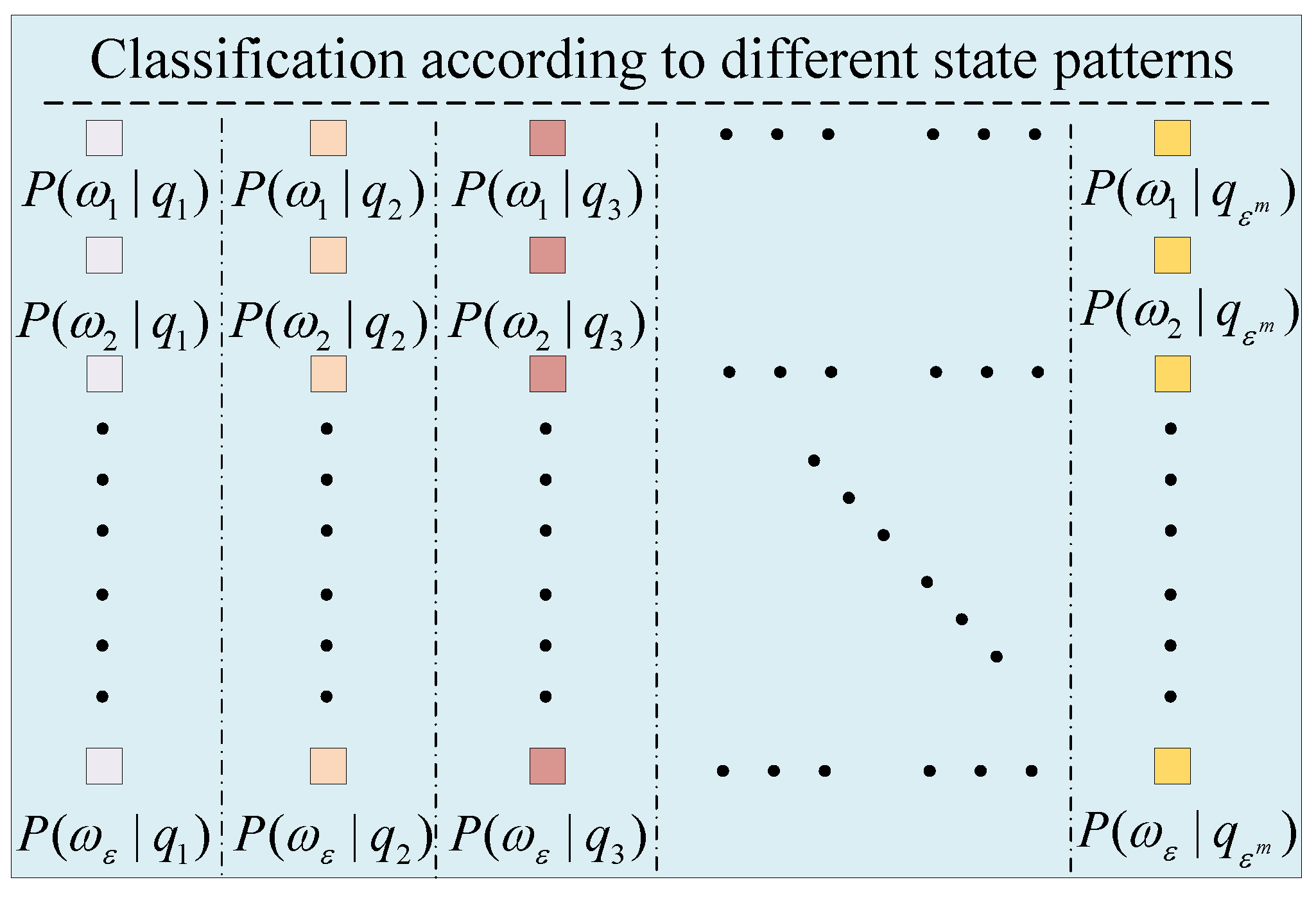
An SCE method is proposed to extract fault information in complex nonlinear time series by classifying the state modes. The information gain of the hydroacoustic signal is increased, which is more conducive to improving the prediction performance.

(2)

An IM algorithm is proposed to detect the initial prediction point, which can avoid missing pivotal information or including unnecessary noise.

(3)

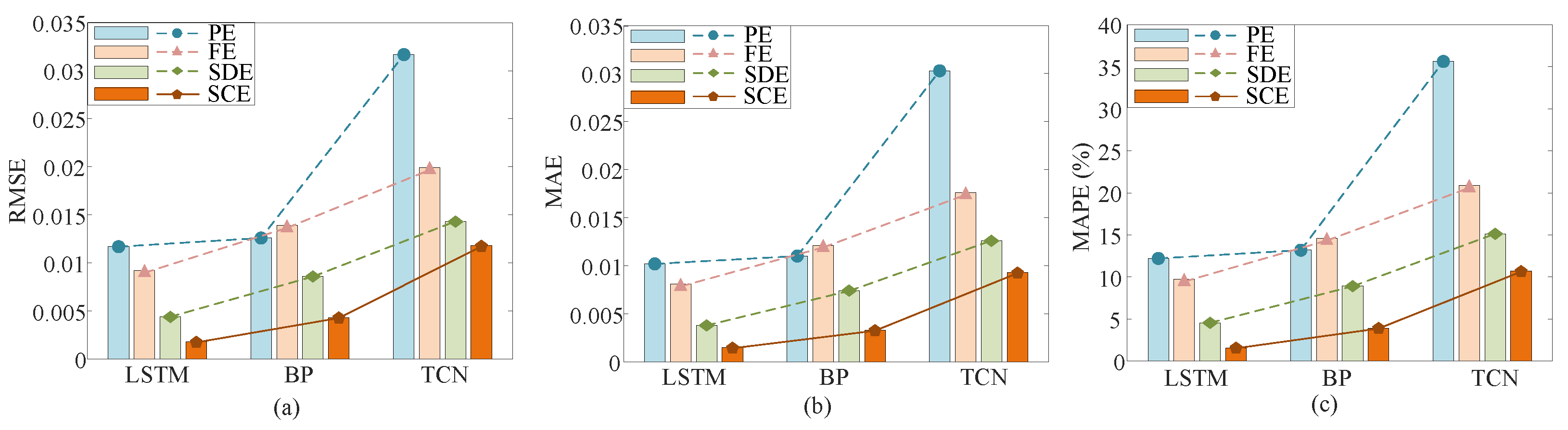
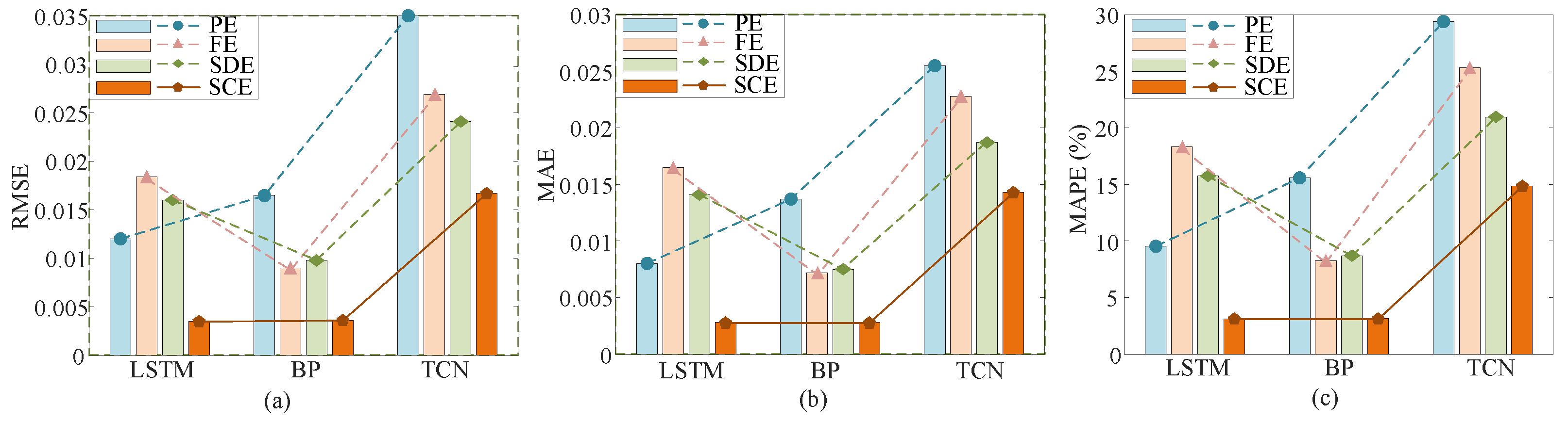
The effectiveness of the proposed method is validated with hydroacoustic signals collected from a hydraulic turbine model test bench. The results of comparisons with different prediction algorithms show that the proposed SCE has excellent trend prediction performance and high precision, as evaluated using RMSE, MAE, and MAPE as performance metrics.

The rest of this article is organized as follows. The problem descriptions of the fault case are mainly described in Section 2. Section 3 is the detailed process of the proposed SCE method. The performance of the proposed method evaluated with field data is presented in Section 4. The conclusions are given in Section 5.

2. Problem Descriptions

The basic characteristics of the hydroacoustic signal in cavitation states and the determination of the initial prediction point are described in detail in the following paragraphs.

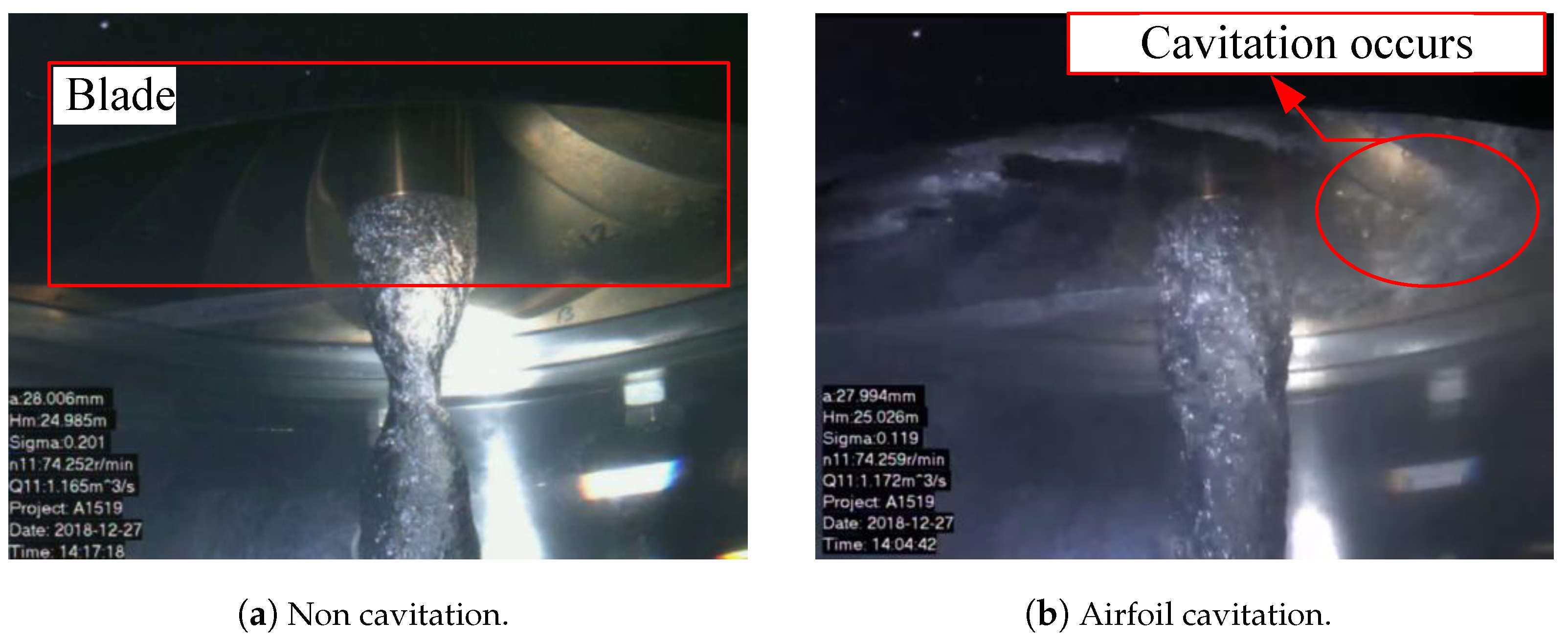
2.1. The Hydroacoustic Signal in Cavitation States

Cavitation is one of the key factors leading to the decrease in equipment performance and structural damage. Accurate prediction of incipient cavitation is crucial to ensure the safe and stable operation of the turbines. However, there are significant challenges in accurately predicting cavitation states. Because of the interference of environmental noise, the uncertainty in the signal increases. The traditional entropy method calculates Shannon entropy in the chaotic state mode. This results in the extracted cavitation features being significantly affected by noise, making it difficult to represent the evolution trend of the cavitation state accurately. Consequently, this leads to low prediction accuracy.

Cavitation includes the formation, expansion, and collapse of bubbles. The pressure at different points in the system where the fluid flows will vary according to the relative motion between the water and the mechanical edges when the turbine operates. According to Equation (1), Bernoulli’s incompressible fluid flow equation, the pressure decreases as the fluid velocity increases. The bubbles in the water expand and grow during the turbine operation [43]. The bubbles will eventually collapse.

$$p+{\displaystyle \frac{1}{2}}\rho v^2+\rho gh=\mathrm{C}$$

(1)

where the p is the fluid local pressure, $\rho$ is the water density, v is the flow velocity, g is the acceleration of gravity, h is the depth at which the fluid is located, and C is a constant.

The power of a hydraulic turbine is defined as

$$P_{out}=M{\displaystyle \frac{2\pi n}{60}}$$

(2)

where M is the torque of the turbine, and n the rotational speed in rpm. The direct result of cavitation is the erosion of turbine components, which reduces the power produced. Under typical conditions, it is expected that when cavitation occurs, the bubble is filled with water vapor, and hence, the pressure in the bubble should be equal to the pressure of saturated vapor $p_v$. To quantify the cavitation states, the cavitation dimensionless number ($\sigma$) is defined as

$$\sigma ={\displaystyle \frac{p_0-p_v}{\rho V_0^2/2}}$$

(3)

where $p_0$ is the reference pressure, which is not disturbed by the flow around the object, $V_0$ the reference flow velocity that is not disturbed by the flow around the object. Different cavitation states correspond to different values of $\sigma$. When the value of the cavitation number is high, cavitation is less likely to occur. On the contrary, when $\sigma$ is small, cavitation is more likely to occur and the degree of cavitation is more serious.

The cavitation number is an important parameter for measuring the cavitation state. A lower cavitation number means that the turbine is closer to cavitation occurring. As the hydraulic turbine transitions from a no-cavitation state to an incipient cavitation state, the cavitation number ($\sigma$) will be gradually reduced from a higher initial value. This reduction continues until it reaches a specific value corresponding to the incipient cavitation number. Therefore, introducing the cavitation number into the prediction process can effectively explain the cavitation states and help describe the dynamic cavitation evolution accurately.

The hydroacoustic signals generated during turbine operation contain various information, including environmental noise, cavitation, and radiation noise. Assuming $y\left(t\right)$ represents the actual hydroacoustic signal, it can be expressed as

$$y\left(t\right)=s\left(t\right)\otimes h\left(t\right)+w\left(t\right)$$

(4)

where $s\left(t\right)$ is the cavitation signal, $h\left(t\right)$ is the impulse response of hydroacoustic multipath channel, ⊗ represents convolution operation, and $w\left(t\right)$ is the environmental noise, mechanical noise, and other noise signals except for the cavitation signal.

In the water, the hydroacoustic signal propagates due to reflection, refraction, and scattering, leading to multipath propagation and multipath effects [44]. There are multiple paths for the sound wave to travel from the transmitting source to the receiver. Each path corresponds to a different delay time, and these paths collectively form the channel’s impulse response. This can result in signal interference, affecting the clarity and accuracy of the signal. Based on the theory of sound rays, the hydroacoustic multipath channel model can be represented as

$$h\left(t\right)=\sum _{i=1}^{N_{\mathrm{c}}}{A}_i\delta (t-{\tau }_i)$$

(5)

where $\delta \left(t\right)$ is the impulse function, $N_{\mathrm{c}}$ the number of sound lines reaching the receiving end, $A_i$ is the i-th sound line amplitude, and ${\tau }_i$ is the transmission delay between the i-th $(i\ne 1)$ sound line and the first one.

The operating environment of the hydraulic turbine is complex and affected by mechanical friction, vibration, and other noises. There are a lot of stochastic non-Gaussian impulsive noises $w\left(t\right)$ in the collected hydroacoustic signal [45]. It is difficult to extract cavitation features due to the interference of impulsive noise and the weak energy of an incipient cavitation. The prediction accuracy will be affected when the ability of the features to characterize the cavitation evolution trend is insufficient. Therefore, extracting more effective cavitation features is the key to predict incipient cavitation accurately.

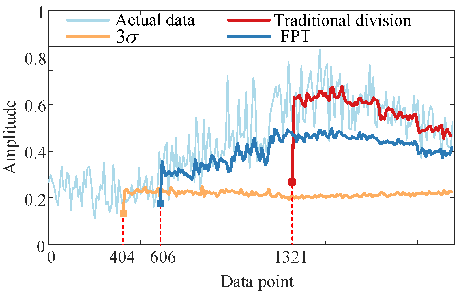
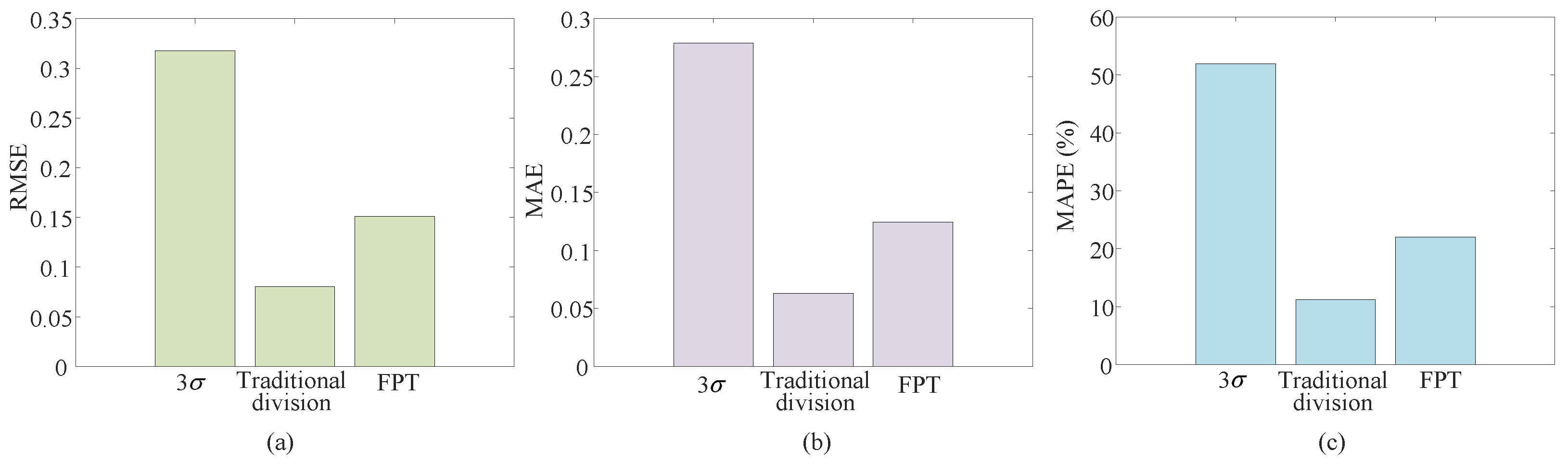
2.2. Determination of Initial Prediction Point

After obtaining the reliable indicator feature of the incipient cavitation to describe the evolution trend of the degree of cavitation, a key step before the prediction is to determine the appropriate initial prediction point [46].

Figure 1 shows the results of the SDE based on the LSTM prediction algorithm. Several methods have been used to determine the initial prediction point, as shown in Figure 1, the 3$\sigma$ criterion of normal distribution in statistics [34,35], the traditional division [36], and first predicting time (FPT) [37]. The 3$\sigma$ criterion and FPT determine the initial prediction point based on the constant threshold. The traditional division determines the initial prediction point based on experience. It can be seen from Figure 1 that the initial prediction point determined by the 3$\sigma$ criterion is too early. This results in predicting before cavitation occurs, and critical information is lost. The prediction curve deviates completely from the actual curve. The initial prediction point determined by FPT is slightly later. The prediction curve of FPT is more realistic than the prediction curve of the 3$\sigma$ criterion. The traditional division determines the latest initial prediction point, and the prediction curve is the closest to the actual curve. However, another issue is that the prediction starts too late, and the incipient cavitation has already occurred. Three different performance metrics, root mean square error (RMSE), mean absolute error (MAE), and mean absolute percentage error (MAPE), are selected to evaluate the prediction performance of the methods. The comparison results in Figure 2 also prove the conclusion in Figure 1. RMSE, MAE, and MAPE of traditional division are the smallest, followed by FPT, and the error of the 3$\sigma$ criterion is the largest. It shows that different initial prediction points significantly affect the prediction accuracy. If the initial prediction point is chosen prematurely, its trend prediction ability is inadequate. The late selection of the initial prediction point may also affect the prediction accuracy due to the inclusion of unnecessary noise. Moreover, Figure 2 shows that due to the weak acoustic energy of the incipient cavitation radiation, its cavitation feature trend is not strictly monotonic. Determining the initial prediction point based on experience or constant thresholds will lead to significant errors.

Although the existing entropy method shows certain effectiveness in some cases, it is still difficult to characterize the evolution trend of cavitation in the face of complex environmental interference accurately. Therefore, accurately predicting incipient cavitation remains challenging. Moreover, the accuracy of the prediction is affected whether it starts too early or too late. Starting too early may result in key information being missed, while starting too late may lead to excess noise being included. To address the above challenges, a method for feature extraction and better initial prediction point determination is required.

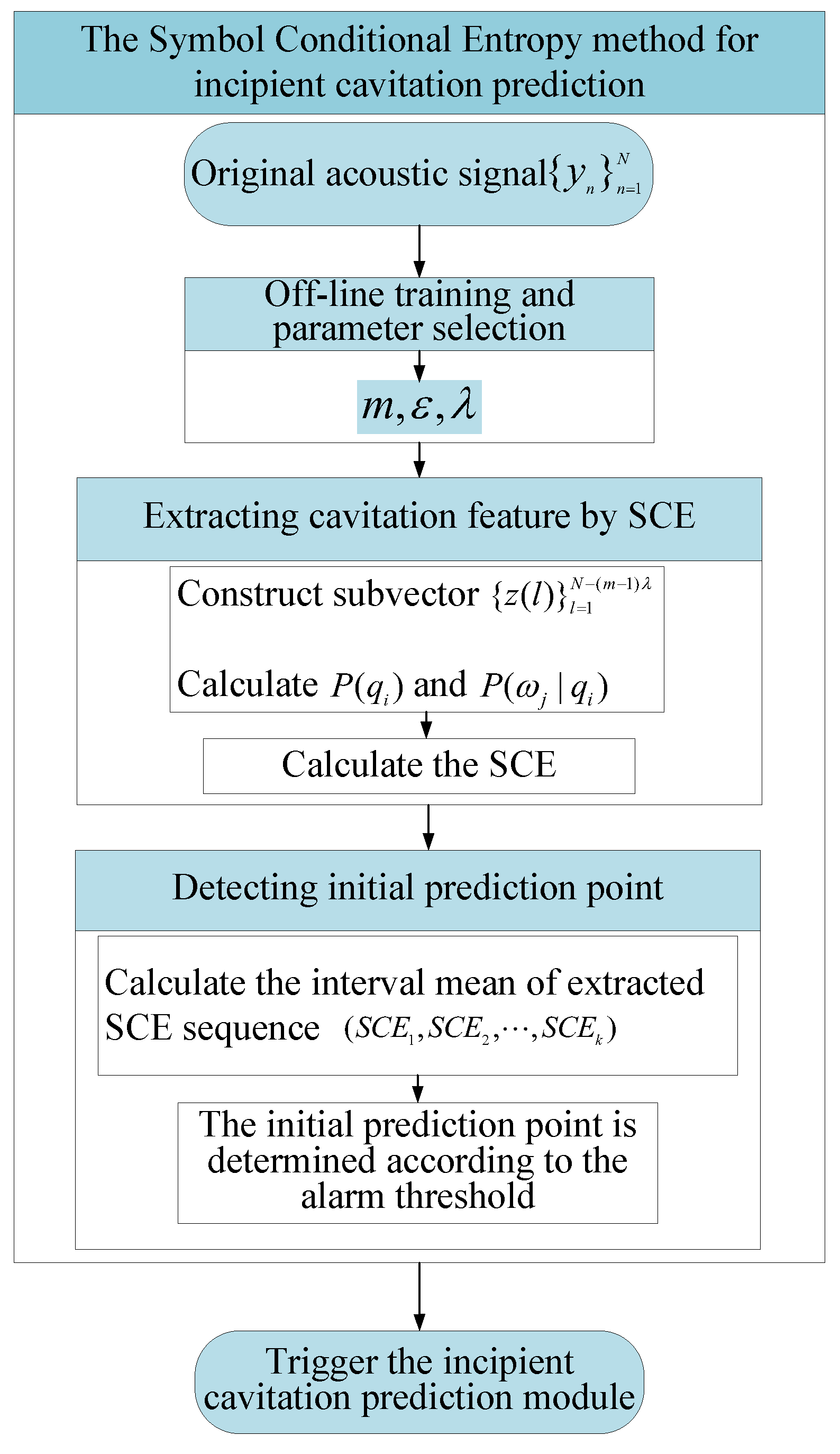
3. The Symbol Conditional Entropy (SCE)

The SCE method is proposed to address the problems of low prediction accuracy due to the difficulty in extracting cavitation features and determining the initial prediction point accurately. The SCE method will be introduced in detail in this section.

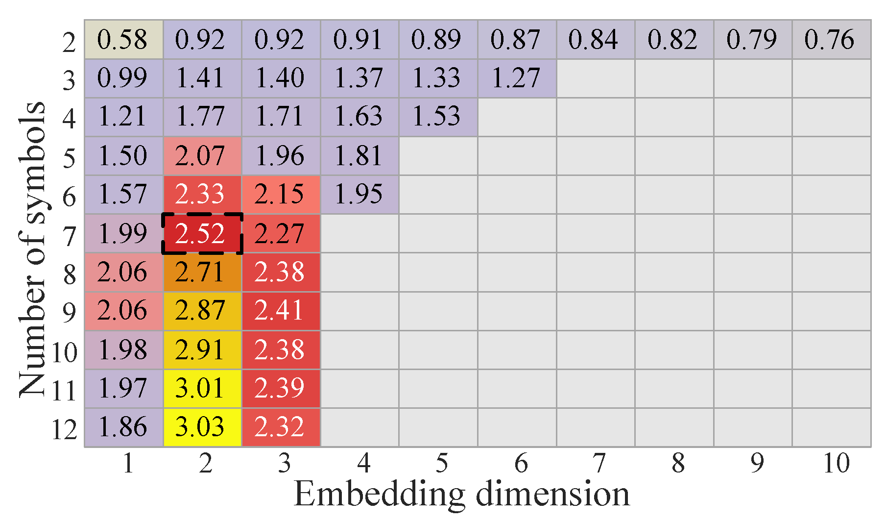
3.1. The SCE Method for Cavitation Feature Extraction

The SCE is developed to extract the fault features from nonlinear time series.

After symbolizing the time series and obtaining the state pattern and state transition matrix, SCE divides the original symbol sequence into different state patterns based on the definition of conditional entropy. After classification, the uncertainty of the entropy decreases, leading to an increase of the information gain, which is helpful for extracting fault information from complex nonlinear time series. Previously, the entropy value was calculated using the Shannon entropy definition by directly using the state pattern and state transition matrix. The information that the state pattern is known is ignored, which leads to greater uncertainty of entropy. Therefore, as shown in Figure 3, state patterns are regarded as known variables, and the original variables are classified according to different state patterns to calculate the SCE.

For a given hydroacoustic signal ${\left\{y_i\right\}}_{i=1}^{\mathrm{N}}$, the original time series is decomposed into intervals with the maximum entropy partitioning (MEP) [47]. The original time series is reconstructed into a symbol sequence $S\left\{s\right(i),i=1,2,\cdots ,\mathrm{N}\}$ by replacing each element $y_n$ with a different symbol ${\omega }_j(j=1,2,\cdots ,\epsilon )$.

Subvectors are constructed by reconstructing symbol sequences. Given the embedding dimension m and the time delay $\lambda$, the reconstructed symbol sequence can be divided into different subvectors as in Equation (6).

$$\left\{z\right(l),z(l+\lambda ),\cdots ,z(l+(m-1)\lambda \left)\right\},l=1,2,\cdots ,N-(m-1)\lambda$$

(6)

The state pattern for each subvectors is unique. Each subvector consists of m components. The reconstructed subvector includes ${\epsilon }^m$ different symbol arrangement state patterns.

The probability of each state pattern $q_i(i=1,2,\cdots ,{\epsilon }^m)$ occurring in all subvectors is

$$P\left(q_i\right)={\displaystyle \frac{\{l:l\le N-(m-1)\lambda ,type\left(S_l\right)=q_i\}}{N-(m-1)\lambda }}$$

(7)

where $type(•)$ is the mapping relationship between symbol and pattern spaces, and $\left|\right|•\left|\right|$ is the total number of items in a given set that meet the mapping relationship. A state pattern matrix can be established: ${[P\left(q_1\right),P\left(q_2\right),\dots ,P\left(q_{{\epsilon }^m}\right)]}_{1\times {\epsilon }^m}$.

The state pattern transition probability of the reconstructed symbol sequence can be calculated as

$$P\left({\omega }_j\right|q_i)={\displaystyle \frac{\{l:l\le N-m\lambda ,type\left(S_l\right)=q_i,S(l+m\lambda )={\omega }_j\}}{N-m\lambda }}$$

(8)

When a state pattern $q_i$ appears, the event that the next symbol appears adjacent to it is called the transition of the state pattern, which changes the complexity of measuring a time series from the amplitude fluctuation to the alternate appearance of the state pattern. The complexity of time series can be measured from a new perspective. Not only are numerical changes considered, but the sequence of transitions between different state patterns is also taken into account. By this method, the dynamic properties in the time series and their intrinsic structure can be captured more comprehensively.

The state pattern transition matrix is defined as

$$\left[\begin{array}{ccc}P\left({\omega }_1\right|q_1)& \dots & P\left({\omega }_{\epsilon }\right|q_1)\\ ⋮& \ddots & ⋮\\ P\left({\omega }_1\right|q_{{\epsilon }^m})& \dots & P\left({\omega }_{\epsilon }\right|q_{{\epsilon }^m})\end{array}\right]$$

(9)

The number of rows of the state pattern transition matrix is the number of state patterns. The number of columns is the number of symbols. As shown in Figure 3, the state pattern transition probability $P\left({\omega }_j\right|q_i)$ is classified according to different state patterns. SCE can be obtained based on the state pattern and state pattern transition matrixes as follows:

$$SCE(y,m,\epsilon ,\lambda )=\sum _{i=1}^{{\epsilon }^m}P\left(q_i\right)H(\omega \mid Q=q_i)$$

(10)

where $H\left(\omega \right|Q=q_i)=$ $-{\displaystyle \sum _{j=1}^{\epsilon }}P\left({\omega }_j\right|Q=q_i)ln\left(P\left({\omega }_j\right|Q=q_i)\right)$.

In Figure 3, each column has the same state pattern, which is $qi$. The elements in each column are the state pattern transition probabilities of different symbols under the state pattern $qi$. The uncertainty of signals can be quantified using entropy values. The larger the entropy value, the greater the uncertainty that is indicated. The information gain is computed as the difference between the entropy before classification and the entropy after classification. Increasing the information gain is beneficial to reduce the uncertainty of the obtained information. The information gain is increased by SCE through the classification of state patterns. This improvement leads to an enhanced capability for extracting cavitation features.

When calculating the state pattern transition probability, the conditional probability is obtained. For example, the probability of $P\left({\omega }_1\right|q_1)$ represents the probability of ${\omega }_1$ occurring in the case of $q_1$, the uncertainty of ${\omega }_1$. State pattern transition probabilities are classified according to different state patterns qi, and the SCE is calculated. The uncertainty of the state pattern is reduced and the information gain is increased.

Lemma 1.

The SCE method reduces the uncertainty and increases the information gain. Let us define the information gain as $Gai{n}_{en}$. $Gai{n}_{en}=SDE-SCE$.

Proof. 

$SDE(y,m,\lambda ,\epsilon )$

$=-{\displaystyle \sum _{i=1}^{{\epsilon }^m}}P\left(q_i\right)·lnP\left(q_i\right)-{\displaystyle \sum _{i=1}^{{\epsilon }^m}}{\displaystyle \sum _{j=1}^{\epsilon }}P\left(q_i\right)ln(P\left(q_i\right)·P({\omega }_j\mid q_i))$

$=-{\displaystyle \sum _{i=1}^{{\epsilon }^m}}P\left(q_i\right)·lnP\left(q_i\right)-{\displaystyle \sum _{i=1}^{{\epsilon }^m}}{\displaystyle \sum _{j=1}^{\epsilon }}P\left(q_i\right)·ln\left(P\left({\omega }_j{q}_i\right)\right)$

Let $P_{\mathrm{A}}=-{\displaystyle \sum _{i=1}^{{\epsilon }^m}}{\displaystyle \sum _{j=1}^{\epsilon }}P\left(q_i\right)lnP\left({\omega }_j{q}_i\right)$, and

$P_{\mathrm{B}}=-{\displaystyle \sum _{i=1}^{{\epsilon }^m}}{\displaystyle \sum _{j=1}^{\epsilon }}P\left(q_i\right)·P\left({\omega }_j\right|q_i)·lnP\left({\omega }_j\right|q_i)$.

Because these two events are not independent, $P\left({\omega }_j{q}_i\right)=P\left({\omega }_j\right|q_i)·P\left(q_i\right)<P\left({\omega }_j\right|q_i)$.

The logarithmic function is monotonically increasing. So, $lnP\left({\omega }_j{q}_i\right)<lnP\left({\omega }_j\right|q_i)<P\left({\omega }_j\right|q_i)·lnP\left({\omega }_j\right|q_i)$. Therefore, $P_{\mathrm{A}}>P_{\mathrm{B}}$. As a result, $Gai{n}_{en}=SDE-SCE>0$. □

Features that characterize the evolution of cavitation can be extracted, which is an important foundation for accurately detecting the initial prediction point. If the extracted features are heavily influenced by noise and have poor monotonicity, they cannot accurately describe the evolution of cavitation. The accuracy of detecting the initial prediction point will also be affected, leading to a decrease in prediction accuracy. The information gain is increased to ensure that the extracted features are more representative, reducing the impact of noise on feature extraction. On this basis, the initial prediction point can be detected in a way that better avoids key information being overlooked and prevents excess noise from being included. Consequently, the initial prediction point is accurately determined, and prediction accuracy is improved.

3.2. The IM Algorithm for Initial Prediction Point Detection

To achieve high-precision incipient cavitation prediction, an IM algorithm is proposed to detect the initial prediction point. The IM algorithm is utilized to define the prediction point, with an emphasis on the cavitation process that occurs after the uncertain prediction points. By using the proposed IM, the extracted indicator feature is converted to an interval mean, which can represent the stage differentiation and avoid misjudging the initial prediction points due to the not strictly monotone indicator features. The mean value in each interval is calculated by the sliding window in the IM. The alarm threshold is determined according to the reliability range of normal distribution in statistics. Based on the alarm threshold, the initial prediction point can be accurately detected to prevent the exclusion of critical information. The detailed steps of the IM are presented hereafter.

Let us assume that the extracted SCE sequence is $(SC{E}_1,SC{E}_2,\cdots ,SC{E}_k)$, and then calculate the mean $A{V}_i$ in each interval through the sliding window:

$$A{V}_i={\displaystyle \frac{{\displaystyle \sum _{j=i}^{i+size-1}}SC{E}_j}{size}}i=1,2,\cdots ,k-size+1$$

(11)

where $size$ is the sliding window size.

The interval mean subsequence is ${[A{V}_1,A{V}_2,\cdots ,A{V}_{k-w_{size}+1}]}_{1\times k-w_{size}+1}$.

The alarm threshold $T_1$ is determined according to the reliability range of normal distribution in statistics. The upper boundary is usually chosen as the observation with an upward trend, so the upper boundary is chosen as the alarm threshold:

$$T_1={\mu }_{A{V}_i}+std$$

(12)

where ${\mu }_{A{V}_i}$ and $std$ are the mean and standard deviation of the interval mean subsequence. The first point above the alarm threshold is the initial prediction point.

3.3. Incipient Cavitation Prediction

The process of feature extraction using the SCE method is depicted in Algorithm 1. The overall framework of the proposed method is depicted in Figure 4.

Algorithm 1 Feature extraction using SCE.

Input: The hydroacoustic signal ${\left\{y_i\right\}}_{i=1}^N$, the parameters $\epsilon ,m,\lambda$. Output: SCE value. 1: ${\left\{y_i\right\}}_{i=1}^N$ is reconstructed into a symbol sequence ${\left\{S_i\right\}}_{i=1}^N$ by MEP. 2: Construct the subvector ${\left\{z\left(l\right)\right\}}_{l=1}^{N-(m-1)\lambda }$. 3: Calculate the probability of each state pattern $P\left(q_i\right)$, and construct the state pattern matrix. 4: Calculate the state pattern transition probability $P({\omega }_j\mid q_i)$ of the reconstructed symbol sequence. 5: Construct the state pattern transition matrix using Equation (9). 6: Calculate the SCE using Equation (10).

The parameters are determined during the off-line stage. The Euclidean Distance (ED) is used to select the optimal parameters. The ED is intended to be utilized with SCE values to calculate the Euclidean Distance between different cavitation states of the turbine. A larger ED indicates higher distinguishability between different cavitation states, indicating a stronger ability of SCE to extract useful information from cavitation noise signals. The SCE values of each sample in the i-th class are $\{SC{E}_i\left(1\right),SC{E}_i\left(2\right),\dots ,SC{E}_i\left(n\right)\}$. The SCE values of each sample in the j-th class are $\{SC{E}_j\left(1\right),SC{E}_j\left(2\right),\dots ,SC{E}_j\left(n\right)\}$. The ED between the i-th and j-th classes is defined as

$$E{D}_{i,j}=\sqrt{\sum _{p=1}^{\mathrm{n}}{\left(SC{E}_i\left(p\right)-SC{E}_j\left(p\right)\right)}^2}$$

(13)

After determining the optimal parameters, the cavitation feature is extracted based on the SCE method. The cavitation feature is extracted to describe the evolution trend of turbine cavitation degree.

The determined initial prediction point triggers the incipient cavitation prediction module. The SCE sequence $(SC{E}_1,SC{E}_2,\cdots ,SC{E}_i)$ and its corresponding cavitation number label $({\sigma }_1,{\sigma }_2,\cdots ,{\sigma }_i)$ before the initial prediction point is input into the network for training. Finally, the prediction label sequence $({{\sigma }^{\prime }}_{i+1},{{\sigma }^{\prime }}_{i+2},\cdots ,{{\sigma }^{\prime }}_k)$ is obtained by using the trained network prediction.

4. Experimental Results and Analysis

In this section, the performance of the proposed SCE is evaluated from the aspects of robustness and monotonicity, and classical entropy algorithms such as PE, FE, and SDE are used as comparison methods. The parameter selection of SCE is also discussed. Finally, the proposed method is applied to the incipient cavitation prediction of an actual turbine.

4.1. Data Description

Real hydroacoustic signals are used to validate the effectiveness of the proposed method. The data are provided by the Harbin Institute of Large Electric Machinery. The hydroacoustic signal data of the airfoil cavitation are obtained through a B&K 8103 hydrophone mounted near 0.3D of the draft tube. The airfoil cavitation is identified as the primary cause of erosion damage to turbine runner blades. Figure 5 shows the phenomenon of both none cavitation and airfoil cavitation on the Francis turbine. It can be seen from Figure 5 that bubbles are observed on the runner blade surfaces during cavitation. The sampling rate is set to 44.1 kHz. To illustrate the reliability of the results, two typical and representative cavitation cases of hydraulic turbines are used for validation. The values of $\sigma$ for each case are shown in

Table 1. The experimental values of $\sigma$ from the hydraulic turbine model test bench.

Operating Condition	None Cavitation										Incipient Cavitation
Case 1	0.250	0.200	0.180	0.150	0.140	0.130	0.120	0.110	0.100	0.09	0.08
Case 2	0.160		0.140		0.120		0.100		0.09		0.08

. In the two cases, the incipient cavitation number is 0.08.

4.2. The Performance Evaluation of the SCE

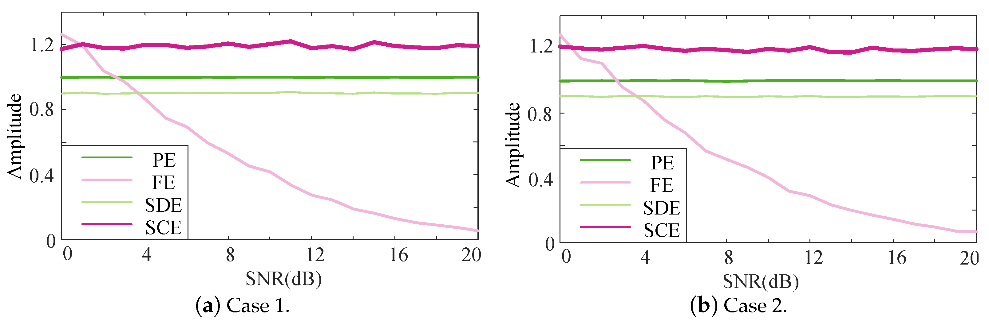
4.2.1. Robustness Test

To evaluate the robustness of the SCE, white Gaussian noise with different signal-to-noise ratios (SNRs: 20:$-1$:0 dB) is added to the hydroacoustic signal. For the parameter settings for SCE and the other comparative entropy algorithms, the embedding dimension, the symbol number, the time delay, and the tolerance are, respectively, set to $m=3$, $\epsilon =6$, $\lambda =1$, and $\gamma =0.15$. $Rob$, an indicator used to quantify the robustness of these four entropy methods, is defined as follows:

$$Rob={\displaystyle \frac{1}{L}}\sum _{j=1}^L{e}^{-{\displaystyle \frac{y_R\left(t_j\right)}{y\left(t_j\right)}}}$$

(14)

where $y_R\left(t_j\right)$ is the trend term obtained by exponential weighted moving smoothing decomposition of the signal sequence, L is the length of the signal, and $y\left(t_j\right)$ is the original signal.

The result is shown in Figure 6. The SCE is almost constant, while the FE monotonically decreases with the increased SNR. The amplitudes of PE and SDE also remain almost constant with increasing SNR. It is indicated that SCE, PE, and SDE are more robust than FE.

A higher value for $Rob$ indicates better robustness. The value range of $Rob$ is [0, 1], and the closer it is to 1, the better the robustness of the method. The $Rob$ results obtained by quantization are shown in

Table 2. Robustness of the different entropy algorithms.

Operating Condition	Methods
	PE	FE	SDE	SCE
Case 1	0.9991	0.3633	0.9976	0.9916
Case 2	0.9994	0.3684	0.9975	0.9915

. The $Rob$ of SCE, PE, and SDE are very close, with values above 0.99. SCE, PE, and SDE are all robust to the noise. In contrast, the $Rob$ of FE is significantly lower than that of SCE, PE, and SDE, indicating that FE is more susceptible to noise interference. The SCE is suitable for extracting features from signals in high-noise environments due to its superior robustness.

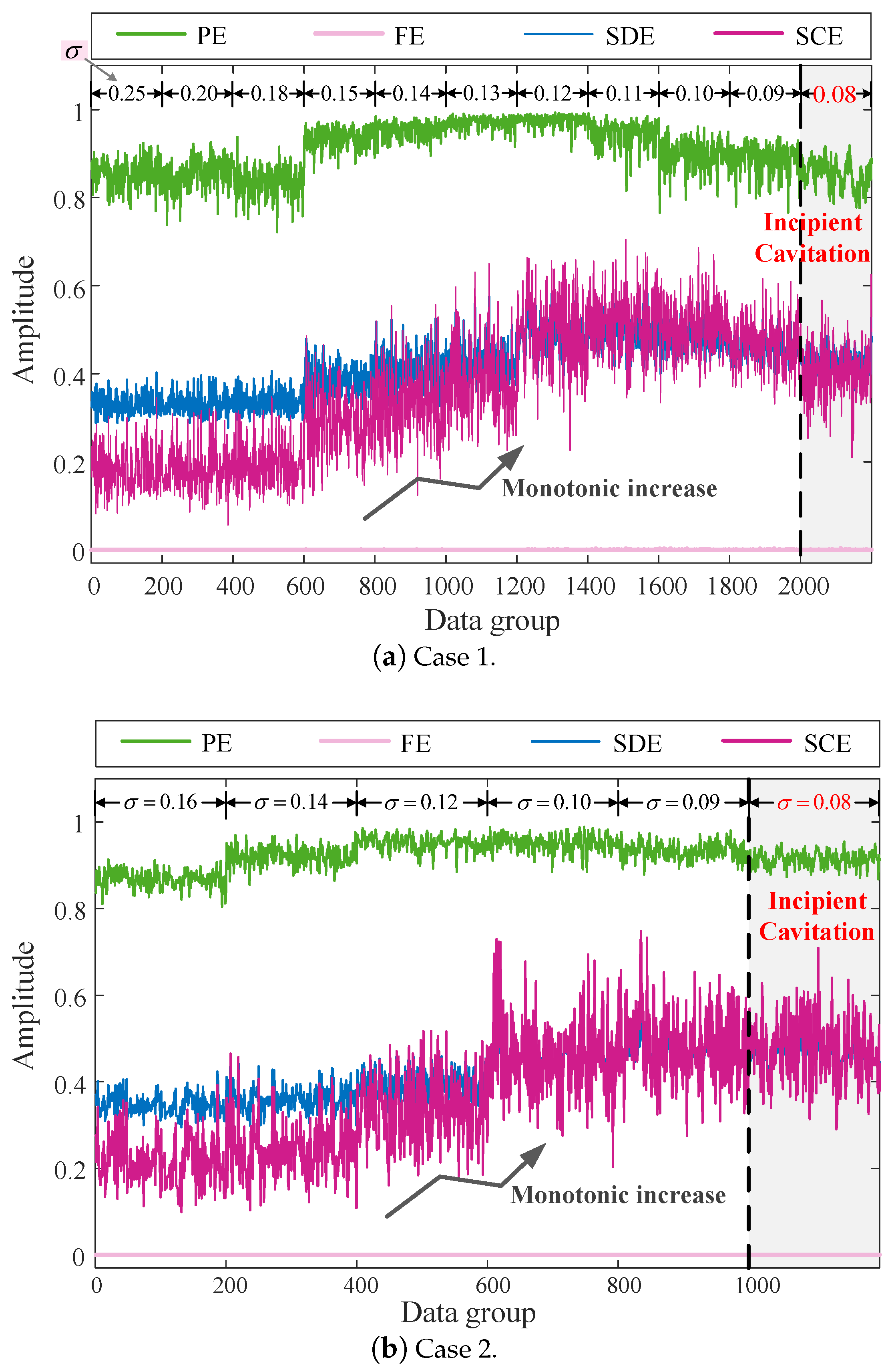
4.2.2. Monotonicity Test

The data were obtained from the hydraulic turbine model test bench under two operating conditions. For each $\sigma$, 200 samples are selected in each sliding window. The entropy of each sample is calculated. If the trend of cavitation evolution can be well characterized by the extracted features, then these features should exhibit a clear trend and monotonicity as the degree of cavitation becomes more severe. As shown in Figure 7, it can be observed that PE and FE do not exhibit a monotonous trend with the gradual increase in the degree of cavitation. For Case 1, the PE curve shows an initial increase followed by a decrease as cavitation becomes more severe. The ability to characterize the cavitation degree using this curve is poor. Additionally, the FE curve is almost a straight line, which fails to describe the evolution of cavitation. While SDE has a slightly better monotonicity, the monotonous trend is still not obvious. By contrast, SCE has a good monotonicity with the increase in the degree of cavitation under the two operating conditions, and the monotonous trend is also more consistent. The monotonicity of the four entropy algorithms is quantified by an index called monotonicity, which is defined as follows:

$$Monotonicity=\sum _{j=2}^{\mathrm{N}}f\left(y_j\right)-f\left(y_{j-1}\right)$$

(15)

where $f\left(y_j\right)$ is the extracted entropy.

The monotonicity of each entropy algorithm for the two operating conditions is shown in

Table 3. Monotonicity of the different entropy algorithms.

Operating Condition	Methods
	PE	FE	SDE	SCE
Case 1	−0.1075	0.00008	0.0715	0.1690
Case 2	−0.0713	0.00002	0.0912	0.1910

. A higher value of $Monotonicity$ indicates better monotonicity. It is obvious that the proposed SCE has a higher positive value. The value of PE is negative for $Monotonicity$ in different cases, indicating that value decreases monotonically as cavitation occurs. However, the $Monotonicity$ value of PE is still lower than that of SCE. The $Monotonicity$ value of FE is much lower than that of PE, SDE, and SCE, which is consistent with the analysis results shown in Figure 7. The monotonicity of FE is significantly lower compared to other entropy methods. Therefore, SCE exhibits the best monotonicity, suggesting that it is better suited for characterizing the trend of cavitation evolution.

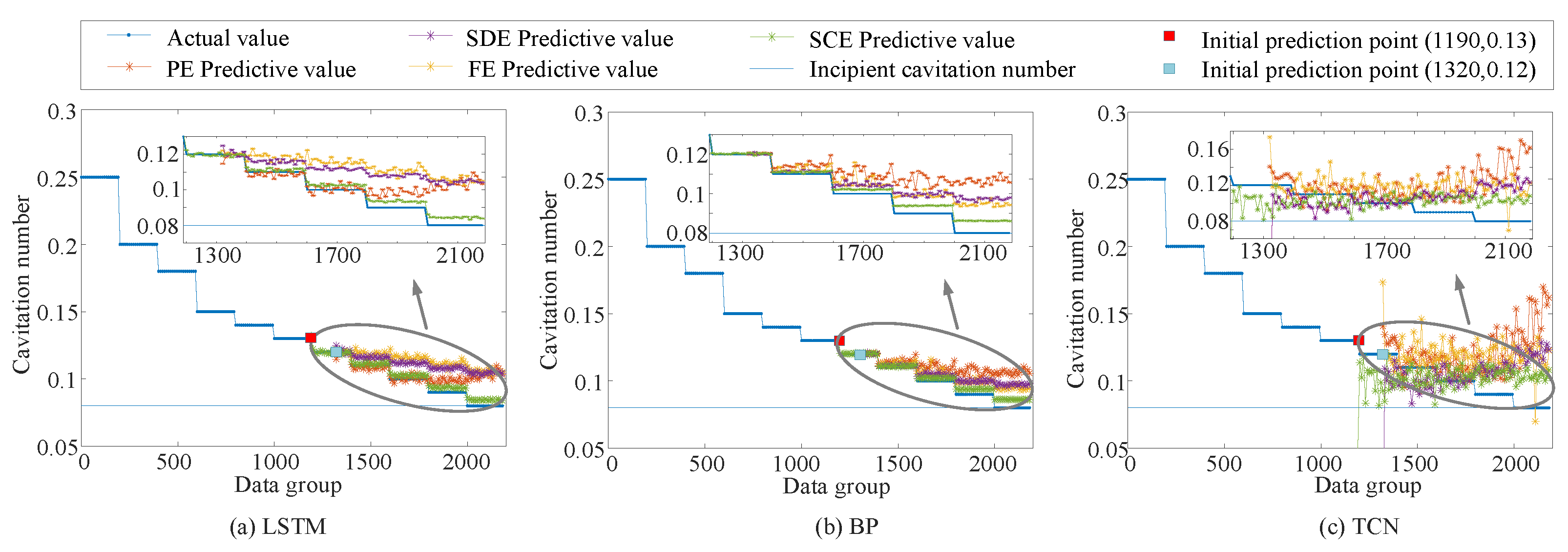
4.3. The Comparison Results of Incipient Cavitation Prediction

It can be concluded from the results in the previous section that the proposed method has superior robustness and monotonicity compared to the other one. The features extracted by the proposed method can characterize the cavitation evolution trend, and then the incipient cavitation can be predicted. The effectiveness of the proposed method will be compared with different entropy algorithms under different prediction algorithms.

The optimal setting of time delay $\lambda$ is studied by using ED. The length of the hydroacoustic signal samples is $L=1024$, with a total of $N=100$ samples, the embedding dimension and the number of symbols are set to $m=3$ and $\epsilon =6$, respectively. The ED between different cavitation states under different time delays is calculated, and the results are shown in

Table 4. The Euclidean Distance between different cavitation states with varying time delay.

$\mathit{\lambda }$	1	2	3	4	5	6
ED	2.1544	2.1505	2.1459	2.1476	2.1486	2.1473

.

It can be observed that changes in the time delay have virtually no impact on the performance of the SCE in Table 4. Therefore, for convenience, the time delay is set to 1.

Then, the optimal embedding dimension and the number of symbols should be determined. The parameters $(\epsilon ,m)$ initialized according to the criterion ${\epsilon }^m<L$ [32]. The number of symbols is set to $\epsilon \in [2,12]$, and the EDs for different cavitation states are calculated and displayed in Figure 8. The results show that the greater the number of symbols, the greater the ED value, that is, the higher the distinguishability of SCE to different cavitation states. More symbols enable a finer division of sequences and more detailed classification, which allows SCE to capture the dynamic changes in signals better. Consequently, different degrees of cavitation can be better represented. Although a larger number of symbols can make the division of the symbol sequence more fine and capture more relevant information in the original data, it will increase the computation burden.

The proposed method is implemented by using Matlab R2022b based on the Windows 11 system and 13th Gen Intel(R) Core(TM) i7-13700H. The calculation time is displayed in

Table 5. Comparison of calculation time.

$\mathit{\epsilon }$	7	8	9	10	11	12
Time (s)	0.2878	0.4417	0.3729	0.9897	1.1046	1.1453

. The results show that the calculation time becomes significantly longer as the number of symbols increases. Considering factors such as computational efficiency and ED, the embedding dimension and the number of symbols are, respectively, set to $m=2$ and $\epsilon =7$. Therefore, the selected parameters are optimal, satisfying distinguishability and calculation time objectives.

The SCE value of the hydroacoustic signal in different cases is calculated. The SCE is used as the feature of incipient cavitation prediction to describe the evolution trend of turbine cavitation intensity. For each $\sigma$, the SCE, PE, FE, and SDE are calculated by using the hydroacoustic data with different cavitation numbers selected by the sliding window, and 200 samples are obtained. The LSTM, BP, and TCN, as classical time series prediction algorithms, are used for comparison for incipient cavitation prediction. Following the classical rule of the data set, 60% is used for training and 40% for testing, respectively. To ensure the fairness of the experiment, the same hyperparameters shown in

Table 6. Hyperparameters for the experiment.

Parameter	Value
$w_{size}$	50
MaxEpochs	300
LearnRateDropPeriod	50
Number of LSTM hidden units	27
Number of TCN numFilters	128
Number of TCN filterSize	3

are used. Simultaneously, RMSE, MAE, and MAPE are used to assess the accuracy of prediction.

Figure 9 shows the prediction results for incipient cavitation by using different entropy algorithms and prediction algorithms for Case 1. The initial prediction point of PE, FE and SDE is (1320, 0.12). The first 1320 points are used for training to predict the last 870 points in Case 1. The initial prediction point found by the IM algorithm is (1190, 0.13). The initial prediction point detected by the IM algorithm is earlier, indicating that the IM algorithm includes key information in the prediction process. The first 1190 feature points are fed into the network for training to predict the last 1000 points in Case 1. As it can be observed from the results for LSTM and BP, the prediction curves of PE, FE, and SDE fail to fit the distribution of the actual feature points. The errors between the predicted and real curves gradually increase. Obviously, the prediction curve of the SCE fits better with the distribution of the actual feature points. The performance of TCN is significantly worse. It can be noted that the proposed SCE method has outstanding trend prediction performance, which is helpful to predict the evolving trend of cavitation degree.

Three performance metrics, RMSE, MAE, and MAPE, are used to evaluate the trend prediction ability of SCE. The comparison results for incipient cavitation prediction in Case 1 are presented in

Table 7. Accuracy comparison for Case 1.

Methods	LSTM			BP			TCN
	RMSE	MAE	MAPE (%)	RMSE	MAE	MAPE (%)	RMSE	MAE	MAPE (%)
PE	0.0117	0.0102	12.23	0.0126	0.0110	13.22	0.0317	0.0303	35.67
FE	0.0092	0.0081	9.72	0.0139	0.0121	14.61	0.0199	0.0176	20.91
SDE	0.0044	0.0038	4.56	0.0086	0.0074	8.92	0.0143	0.0126	15.13
Proposed SCE	0.0018	0.0015	1.59	0.0043	0.0033	3.93	0.0118	0.0093	10.69

and Figure 10. The RMSE, MAE, and MAPE of SCE are the smallest under the different prediction algorithms. However, the RMSE, MAE, and MAPE of PE, FE, and SDE are higher than those of SCE. In addition, the proposed method has the smallest incipient cavitation prediction error under the LSTM algorithm. It can be seen from Table 7 that the prediction accuracy under the LSTM algorithm is superior to that of BP and TCN, indicating that the predictive performance of LSTM is the best. The RMSE, MAE, and MAPE of the proposed SCE decreased by 84.62%, 85.29%, and 87% compared with the PE method.

Figure 11 shows the prediction results of incipient cavitation by using different entropy algorithms and prediction algorithms in Case 2. The initial prediction point of PE, FE and SDE is (720, 0.1). The first 720 points are used for training to predict the last 470 points in Case 2. The initial prediction point detected by the IM algorithm is (609, 0.1). The first 609 feature points are fed into the network for training to predict the last 581 points. As it can be seen from the results for LSTM and BP, the prediction curves of FE and PE failed to fit the distribution of the real feature points. The errors between the predicted and real curves become larger gradually. Although the prediction curve of SDE fits the distribution of real data better than that of FE and PE, the error is still large. The prediction curve of the proposed SCE successfully fits the real feature point distribution. The prediction performance of TCN is obviously worse than that of LSTM and BP. Nevertheless, the prediction curve of the SCE is still the closest to the true distribution. The proposed SCE method is excellent in predicting the cavitation evolving trend.

Likewise, the three performance metrics RMSE, MAE, and MAPE are used to evaluate the trend prediction ability of SCE. The comparison results of incipient cavitation prediction in Case 2 are shown in

Table 8. Accuracy comparison for Case 2.

Methods	LSTM			BP			TCN
	RMSE	MAE	MAPE (%)	RMSE	MAE	MAPE (%)	RMSE	MAE	MAPE (%)
PE	0.0120	0.0080	9.53	0.0165	0.0137	15.57	0.0350	0.0255	29.39
FE	0.0184	0.0165	18.34	0.0090	0.0072	8.26	0.0269	0.0228	25.32
SDE	0.0160	0.0141	15.78	0.0098	0.0075	8.7	0.0241	0.0187	20.95
Proposed SCE	0.0035	0.0028	3.11	0.0036	0.0028	3.16	0.0167	0.0143	14.88

and Figure 12. Compared with other entropy methods, the proposed SCE method has minimal error under the different prediction algorithms. The RMSE, MAE, and MAPE of PE, FE, and SDE are higher than those of SCE. The proposed SCE method has the smallest RMSE, MAE and MAPE for incipient cavitation prediction using the LSTM prediction algorithm. It can be seen from Table 8 that the prediction accuracy under the LSTM algorithm is superior to that of BP and TCN, indicating that the predictive performance of LSTM is the best.

It can be noted that the proposed SCE method has outstanding trend prediction performance, which is helpful to predict the evolving trend of cavitation. The operators can adjust the parameters in time when the cavitation degree becomes severe to prevent greater damage to the equipment. Therefore, the proposed method is suitable for the prediction of the incipient cavitation of hydraulic turbines in practical engineering.

5. Conclusions and Perspectives

A Symbol Conditional Entropy feature extraction method is proposed to analyze hydroacoustic signals. Aiming to solve the problems that the radiation acoustic energy of incipient cavitation is weak and the extracted cavitation features are easily submerged by noise, this method can extract the features that can effectively characterize the cavitation evolution trend. To avoid missing key information or including noise, an interval mean algorithm is proposed to detect the initial prediction point. The features that can represent the cavitation evolution trend are effectively extracted by SCE, and the initial prediction point is determined by the IM algorithm. Thus, the prediction accuracy can be significantly improved. The main conclusions of this article are as follows:

(1)

By classifying state patterns, the SCE method can reduce the uncertainty of information and increase the information gain of the hydroacoustic signal. The prediction performance has been enhanced due to the improved capability to extract cavitation features from complex and nonlinear time series. The RMSE, MAE, and MAPE of the proposed SCE decreased by 84.62%, 85.29%, and 87% compared with the PE method.

(2)

The SCE is used to extract cavitation features from real-time signals effectively, and the initial prediction point is determined using the IM algorithm for trend prediction. The detection of the initial prediction point can focus on cavitation information, which is useful for predicting the evolution trend. The prediction accuracy is improved consequently.

(3)

The proposed SCE is used to predict the incipient cavitation of the hydroacoustic signal collected from a hydraulic turbine test bench. The results show that the proposed method is superior to other used entropy algorithms in fitting the distribution of real feature points and predicting accuracy with different prediction algorithms.

The proposed SCE method also exhibited superior robustness and monotonicity, which are helpful in describing the evolution degree of cavitation. The experimental results showed that the proposed SCE method has outstanding trend prediction performance, high accuracy, and effectiveness. It is suitable for the prediction of the incipient cavitation of hydraulic turbines in practical engineering. This means automatic monitoring can be implemented, and an alert can be triggered when the prediction curve approaches the threshold.

In future works, it will be important to study the optimal setting of symbols and other parameters in different devices to improve the generalizability of the method. This method presents a promising and comprehensive solution for cavitation prediction in hydraulic turbines, with significant potential for engineering applications.

References

1. Zhou, T.; Kao, S.C.; Xu, W.; Gangrade, S.; Voisin, N. Impacts of climate change on subannual hydropower generation: A multi-model assessment of the United States federal hydropower plant. Environ. Res. Lett. 2023, 18, 034009. [Google Scholar] [CrossRef]
2. Kumar, K.; Saini, R.P. A review on operation and maintenance of hydropower plants. Sustain. Energy Technol. Assess. 2022, 49, 101704. [Google Scholar] [CrossRef]
3. Goyal, R.; Gandhi, B.K. Review of hydrodynamics instabilities in Francis turbine during off-design and transient operations. Renew. Energy 2018, 116, 697–709. [Google Scholar] [CrossRef]
4. Yu, A.; Tang, Y.; Tang, Q.; Cai, J.; Zhao, L.; Ge, X. Energy analysis of Francis turbine for various mass flow rate conditions based on entropy production theory. Renew. Energy 2022, 183, 447–458. [Google Scholar] [CrossRef]
5. Feng, J.; Zhao, N.; Zhu, G.; Wu, G.; Li, Y.; Luo, X. Cavitation identification in a hydraulic bulb turbine based on vibration and pressure fluctuation measurements. Mech. Syst. Signal Process. 2024, 208, 111042. [Google Scholar] [CrossRef]
6. Kadivar, E.; Timoshevskiy, M.V.; Nichik, M.Y.; el Moctar, O.; Schellin, T.E.; Pervunin, K.S. Control of unsteady partial cavitation and cloud cavitation in marine engineering and hydraulic systems. Phys. Fluids 2020, 32, 052108. [Google Scholar] [CrossRef]
7. Murovec, J.; Curovic, L.; Novakovic, T.; Prezelj, J. Psychoacoustic approach for cavitation detection in centrifugal pumps. Appl. Acoust. 2020, 165, 107323. [Google Scholar] [CrossRef]
8. Yan, Z.; Liu, J.; Chen, B.; Cheng, X.; Yang, J. Fluid cavitation detection method with phase demodulation of ultrasonic signal. Appl. Acoust. 2015, 87, 198–204. [Google Scholar] [CrossRef]
9. Firly, R.; Inaba, K.; Triawan, F.; Kishimoto, K.; Hayabusa, K.; Nakamoto, H. Numerical prediction of cavitation damage based on shock-induced single bubble collapse near solid surfaces. Eur. J. Mech. B-Fluids 2023, 98, 143–160. [Google Scholar] [CrossRef]
10. Favrel, A.; Pereira Junior, J.G.; Landry, C.; Mueller, A.; Yamaishi, K.; Avellan, F. Dynamic modal analysis during reduced scale model tests of hydraulic turbines for hydro-acoustic characterization of cavitation flows. Mech. Syst. Signal Process. 2019, 117, 81–96. [Google Scholar] [CrossRef]
11. Mousmoulis, G.; Yiakopoulos, C.; Aggidis, G.; Antoniadis, I.; Anagnostopoulos, I. Application of Spectral Kurtosis on vibration signals for the detection of cavitation in centrifugal pumps. Appl. Acoust. 2021, 182, 108289. [Google Scholar] [CrossRef]
12. Kan, K.; Binama, M.; Chen, H.; Zheng, Y.; Zhou, D.; Su, W.; Muhirwa, A. Pump as turbine cavitation performance for both conventional and reverse operating modes: A review. Renew. Sustain. Energy Rev. 2022, 168, 112786. [Google Scholar] [CrossRef]
13. Tiwari, G.; Kumar, J.; Prasad, V.; Patel, V.K. Utility of CFD in the design and performance analysis of hydraulic turbines—A review. Energy Rep. 2020, 6, 2410–2429. [Google Scholar] [CrossRef]
14. Karaalioglu, M.S.; Bal, S. Performance prediction of cavitating marine current turbine by BEMT based on CFD. Ocean. Eng. 2022, 255, 111221. [Google Scholar] [CrossRef]
15. Brijkishore; Khare, R.; Prasad, V. Prediction of cavitation and its mitigation techniques in hydraulic turbines—A review. Ocean. Eng. 2021, 221, 108512. [Google Scholar] [CrossRef]
16. Sun, H.; Si, Q.; Chen, N.; Yuan, S. HHT-based feature extraction of pump operation instability under cavitation conditions through motor current signal analysis. Mech. Syst. Signal Process. 2020, 139, 106613. [Google Scholar] [CrossRef]
17. Wu, Y.; Zhu, D.; Tao, R.; Xiao, R.; Liu, W. Analysis of two-phase flow in cavitation condition of pump-turbine based on dynamic mode decomposition method in turbine mode. J. Energy Storage 2022, 56, 106107. [Google Scholar] [CrossRef]
18. Zhu, Y.; Li, G.; Tang, S.; Wang, R.; Su, H.; Wang, C. Acoustic signal-based fault detection of hydraulic piston pump using a particle swarm optimization enhancement CNN. Appl. Acoust. 2022, 192, 108718. [Google Scholar] [CrossRef]
19. Sha, Y.; Faber, J.; Gou, S.; Liu, B.; Li, W.; Schramm, S.; Stoecker, H.; Steckenreiter, T.; Vnucec, D.; Wetzstein, N.; et al. A multi-task learning for cavitation detection and cavitation intensity recognition of valve acoustic signals. Eng. Appl. Artif. Intell. 2022, 113, 104904. [Google Scholar] [CrossRef]
20. Kang, Z.; Feng, C.; Liu, Z.; Cang, Y.; Gao, S. Analysis of the incipient cavitation noise signal characteristics of hydroturbine. Appl. Acoust. 2017, 127, 118–125. [Google Scholar] [CrossRef]
21. Feng, J.; Men, Y.; Zhu, G.; Li, Y.; Luo, X. Cavitation detection in a Kaplan turbine based on multifractal detrended fluctuation analysis of vibration signals. Ocean. Eng. 2022, 263, 112232. [Google Scholar] [CrossRef]
22. Feng, J.; Liu, B.; Luo, X.; Zhu, G.; Li, K.; Wu, G. Experimental investigation on characteristics of cavitation-induced vibration on the runner of a bulb turbine. Mech. Syst. Signal Process. 2023, 189, 110097. [Google Scholar] [CrossRef]
23. Yang, C.; Gabbouj, M.; Jia, M.; Li, Z. Hierarchical Symbol Transition Entropy: A Novel Feature Extractor for Machinery Health Monitoring. IEEE Trans. Ind. Inform. 2022, 18, 6131–6141. [Google Scholar] [CrossRef]
24. Huo, Z.; Martinez-Garcia, M.; Zhang, Y.; Yan, R.; Shu, L. Entropy Measures in Machine Fault Diagnosis: Insights and Applications. IEEE Trans. Instrum. Meas. 2020, 69, 2607–2620. [Google Scholar] [CrossRef]
25. Yang, C.; Jia, M. Hierarchical multiscale permutation entropy-based feature extraction and fuzzy support tensor machine with pinball loss for bearing fault identification. Mech. Syst. Signal Process. 2021, 149, 107182. [Google Scholar] [CrossRef]
26. Minhas, A.S.; Singh, G.; Singh, J.; Kankar, P.K.; Singh, S. A novel method to classify bearing faults by integrating standard deviation to refined composite multi-scale fuzzy entropy. Measurement 2020, 154, 107441. [Google Scholar] [CrossRef]
27. Li, Y.X.; Li, Y.A.; Chen, Z.; Chen, X. Feature Extraction of Ship-Radiated Noise Based on Permutation Entropy of the Intrinsic Mode Function with the Highest Energy. Entropy 2016, 18, 393. [Google Scholar] [CrossRef]
28. Liu, X.; Tang, Z.; Cui, H.; Wang, C. MMC-HVDC grids transmission line protection method: Based on permutation entropy algorithm. Int. J. Electr. Power Energy Syst. 2024, 162, 110296. [Google Scholar] [CrossRef]
29. Saravanan, B.; Mohanraj, V.; Senthilkumar, J. A fuzzy entropy technique for dimensionality reduction in recommender systems using deep learning. Soft Comput. 2019, 23, 2575–2583. [Google Scholar] [CrossRef]
30. Hou, S.; Zheng, J.; Pan, H.; Feng, K.; Liu, Q.; Ni, Q. Multivariate multi-scale cross-fuzzy entropy and SSA-SVM-based fault diagnosis method of gearbox. Meas. Sci. Technol. 2024, 35, 056102. [Google Scholar] [CrossRef]
31. Zhou, X.; Yuan, R.; Lv, Y.; Li, B.; Fu, S.; Li, H. Hierarchical Multiscale Fluctuation-Based Symbolic Fuzzy Entropy: A Novel Tensor Health Indicator for Mechanical Fault Diagnosis. IEEE Sens. J. 2025, 25, 5013–5030. [Google Scholar] [CrossRef]
32. Li, Y.; Yang, Y.; Li, G.; Xu, M.; Huang, W. A fault diagnosis scheme for planetary gearboxes using modified multi-scale symbolic dynamic entropy and mRMR feature selection. Mech. Syst. Signal Process. 2017, 91, 295–312. [Google Scholar] [CrossRef]
33. Yang, C.; Jia, M.; Li, Z.; Gabbouj, M. Enhanced hierarchical symbolic dynamic entropy and maximum mean and covariance discrepancy-based transfer joint matching with Welsh loss for intelligent cross-domain bearing health monitoring. Mech. Syst. Signal Process. 2022, 165, 108343. [Google Scholar] [CrossRef]
34. Chen, Z.; Xia, T.; Li, Y.; Pan, E. A hybrid prognostic method based on gated recurrent unit network and an adaptive Wiener process model considering measurement errors. Mech. Syst. Signal Process. 2021, 158, 107785. [Google Scholar] [CrossRef]
35. Li, N.; Lei, Y.; Lin, J.; Ding, S.X. An Improved Exponential Model for Predicting Remaining Useful Life of Rolling Element Bearings. IEEE Trans. Ind. Electron. 2015, 62, 7762–7773. [Google Scholar] [CrossRef]
36. Sang, L.; Xu, Y.; Long, H.; Hu, Q.; Sun, H. Electricity Price Prediction for Energy Storage System Arbitrage: A Decision-Focused Approach. IEEE Trans. Smart Grid 2022, 13, 2822–2832. [Google Scholar] [CrossRef]
37. Li, N.; Xu, P.; Lei, Y.; Cai, X.; Kong, D. A self-data-driven method for remaining useful life prediction of wind turbines considering continuously varying speeds. Mech. Syst. Signal Process. 2022, 165, 108315. [Google Scholar] [CrossRef]
38. Liu, Q.; Xie, C.; Cheng, B. Butterfly valve erosion prediction based on LSTM network. Flow Meas. Instrum. 2024, 98, 102652. [Google Scholar] [CrossRef]
39. Wu, Y.; Tao, R.; Zhu, D.; Xiao, R. Analysis and prediction of force characteristics of tubular turbine based on Hankel-DMD-LSTM. Eng. Appl. Comput. Fluid Mech. 2025, 19, 2443122. [Google Scholar] [CrossRef]
40. Wang, Y.; Shao, J.; Yang, F.; Zhu, Q.; Zuo, M. Optimization design of centrifugal pump cavitation performance based on the improved BP neural network algorithm. Measurement 2025, 245, 116553. [Google Scholar] [CrossRef]
41. Zhao, Z.; Lin, W. Short-term electric load forecasting based on empirical wavelet transform and temporal convolutional network. IET Gener. Transm. Distrib. 2024, 18, 1672–1683. [Google Scholar] [CrossRef]
42. Li, Y.; Xiao, L.; Wei, H.; Li, D.; Li, X. A Comparative Study of LSTM and Temporal Convolutional Network Models for Semisubmersible Platform Wave Runup Prediction. J. Offshore Mech. Arct. Eng.-Trans. ASME 2025, 147, 011202. [Google Scholar] [CrossRef]
43. Shamsuddeen, M.M.; Park, J.; Choi, Y.S.; Kim, J.H. Unsteady multi-phase cavitation analysis on the effect of anti-cavity fin installed on a Kaplan turbine runner. Renew. Energy 2020, 162, 861–876. [Google Scholar] [CrossRef]
44. Ma, C.; Wang, L.; Gao, J.; Cui, Y.; Peng, C.; Zhang, S. Time of arrival estimation for underwater acoustic signal using multi-feature fusion. Appl. Acoust. 2023, 211, 109475. [Google Scholar] [CrossRef]
45. Wang, J.; Li, J.; Yan, S.; Shi, W.; Yang, X.; Guo, Y.; Gulliver, T.A. A Novel Underwater Acoustic Signal Denoising Algorithm for Gaussian/Non-Gaussian Impulsive Noise. IEEE Trans. Veh. Technol. 2021, 70, 429–445. [Google Scholar] [CrossRef]
46. Yang, L.; Wang, Z.; Li, Y.; Dong, L.; Du, W.; Wang, J.; Zhang, X.; Shi, H. Two-stage prediction technique for rolling bearings based on adaptive prediction model. Mech. Syst. Signal Process. 2024, 206, 110931. [Google Scholar] [CrossRef]
47. Rajagopalan, V.; Ray, A. Symbolic time series analysis via wavelet-based partitioning. Signal Process. 2006, 86, 3309–3320. [Google Scholar] [CrossRef]
Figure 1. Prediction results for different initial prediction points.
Jmse 13 00538 g001
Figure 2. Comparison of prediction performance (a) RMSE (b) MAE (c) MAPE.
Jmse 13 00538 g002
Figure 3. The classification of state pattern transition probability.
Jmse 13 00538 g003
Figure 4. Flowchart of the proposed SCE method.
Jmse 13 00538 g004
Figure 5. Phenomenon of (a) non-cavitation and (b) airfoil cavitation on Francis turbines.
Jmse 13 00538 g005
Figure 6. Robustness of different entropy algorithms to signal-to-noise ratio change.
Jmse 13 00538 g006
Figure 7. Monotonicity of different entropy algorithms to cavitation degree change.
Jmse 13 00538 g007
Figure 8. ED for different parameters, m and ε .
Jmse 13 00538 g008
Figure 9. Prediction results of the different methods for Case 1.
Jmse 13 00538 g009
Figure 10. Comparison of different methods for Case 1 (a) RMSE (b) MAE (c) MAPE.
Jmse 13 00538 g010
Figure 11. Prediction results of the different methods for Case 2.
Jmse 13 00538 g011
Figure 12. Comparison of different methods for Case 2 (a) RMSE (b) MAE (c) MAPE.
Jmse 13 00538 g012