Variability in Diurnal Internal Tides and Near-Inertial Waves in the Southern South China Sea Based on Mooring Observations

Abstract

Temporal variations in diurnal internal tides (ITs) and near-inertial waves (NIWs) in the southern South China Sea (SCS) are characterized, based on two 13-month moored current observations. Diurnal ITs, dominated by O₁ and K₁, are found to exhibit spring–neap cycles of about 14 days and significant seasonal variations. The incoherent components explain 54% and 56% of the total energy in the diurnal band, which further complicates its temporal variabilities. As for NIWs, wind energy input serves as the primary energy source and three strong events are observed. Tropical cyclone RAI passed through two moorings during the event 1 period, and triggered a peak near-inertial kinetic energy of 19.55 J m⁻³ (18.82 J m⁻³) at two moorings. After generation, the NIWs propagated downward to around 300 m, becoming the most intense event observed at DA2. In contrast, the NIWs response to tropical cyclone NOCK’s passage during event 3 was relatively weaker. The near-inertial KE generated by NOCK was confined to depths shallower than 150 m, with the average near-inertial KE being only 85% (52%) of that during event 1 for two moorings, despite the near-inertial energy input from NOCK being nearly 400% that of RAI. The modulation of background vorticity is considered the primary factor resulting in the difference in intensity of two NIW events. The penetrating depth of NIWs under the modulation of anticyclonic eddies was more than twice that under the cyclonic eddies. Furthermore, the strongest NIWs during event 2 that were observed below 350 m at mooring 2 (183% stronger than average) were also related to a strong anticyclonic eddy.

1. Introduction

Internal waves occur in stratified ocean waters with a frequency that is between the local inertial frequency and the buoyancy frequency [1,2], which are the major drivers of diapycnal mixing in the global ocean, and play an important role in different climate relevant processes, such as the transport of heat, and nutrients [2,3,4]. It has been demonstrated that the breaking of internal waves is thought to supply 2.1 TW of energy into diapycnal mixing to maintain abyssal stratification, making it a major driver of global meridional overturning circulation [5]. Internal tides (ITs) and near-inertial internal waves (NIWs) are the two most active fluctuations in the internal wave spectrum, serving as a bridge between the large/mesoscale dynamic processes and turbulence mixing [3,5,6]. ITs are usually generated when barotropic tidal currents flow over rough topographical features, such as the continental shelf break, or ridges [7]. For NIWs, tropical cyclones are one of the most efficient energy sources [8]. Wind stress impulses or fluctuations with frequencies in the near-inertial band can resonantly force inertial motions to occur in the surface mixed layer in addition to sea surface temperature cooling, then NIWs are generated [9,10,11,12].

The South China Sea (SCS), known as the largest marginal sea in the Western Pacific, features a highly complex bathymetry, encompassing extensive continental shelves and deep ocean basins, a strong wind field, and frequent typhoon passages, hence, the internal waves in the SCS are some of the strongest documented in global oceans [2,13]. For ITs, the Luzon Strait, one of the world’s most important sources of IT generation due to its two-ridge system and strong barotropic tides, contributes approximately 90% and 74% of the baroclinic energy for M₂ and K₁ in the SCS [14,15]. After they are generated, high-mode ITs usually dissipate locally due to their strong shear instabilities [16,17]. Meanwhile, low-mode diurnal ITs can propagate southwestward over 1600 km, reaching the southern SCS [15]. As for semidiurnal ITs, they bifurcate into two beams and radiate west to north mainly [18]. Liang [19] showed that the ITs in the northern SCS generated at the Luzon Strait have a time-varying characteristic of spring–neap oscillations of about 14 days and seasonal variations of enhancement in summer. During the process of ITs’ propagation, the phase and amplitude are influenced by the background field, the buoyancy frequency and other factors, resulting in a decrease in the proportion of the coherent part and an increase in the proportion of the incoherent part of ITs, which shows randomness and unpredictability [20,21]. Previous studies [2,22] revealed that the diurnal ITs in the SCS are more susceptible to the influence of multiscale ocean dynamic processes than semidiurnal ITs, resulting in more complicated paths and a wider scope, which further increases the difficulty of their simulation and prediction.

As for NIWs, the SCS is adjacent to the main development region of Western Pacific typhoons, with approximately 12.7 typhoons passing through annually [23,24]. Together with the summer monsoons, strong winds inject significant energy into NIWs [25]. Generally, the magnitude of wind-induced NIWs in the northern SCS varies from 10 to 40 cm/s, which can persist for several days before decaying after the passage of the TC [26,27]. Compared with ITs, the NIWs are more intermittent, which makes the spatial and temporal distributions of the NIWs in the SCS more complicated [8,28,29,30,31]. Previous studies [31,32,33,34,35] show that NIWs are more likely to interact with the mesoscale eddies than ITs owing to their slower group velocities. When NIWs are generated inside anticyclonic eddies with a negative relative vorticity (ζ), the effective Coriolis frequency (${\mathrm{f}}_{\mathrm{e}\mathrm{f}\mathrm{f}}=\mathrm{f}+\mathsf{\zeta }/2$) of the NIWs is lower than the local inertial frequency [36], leading to NIWs being trapped within anticyclonic eddies while being repelled away from cyclonic eddies in both horizontal and vertical directions. Anticyclonic eddies can serve as an important channel for directing energy from the mixed layer to the deeper layer [1,34,37]. Xu et al. [38] observed redshift NIWs concentrated within an anticyclonic eddy core (200 m to 300 m) with current amplitudes exceeding 0.2 m s⁻¹. Under the trapping effect of the anticyclonic eddy, near-inertial kinetic energy usually decays roughly in a Gaussian form along the eddy radius and propagates southwestward for hundreds of kilometers together with the eddy [38]. In addition, NIWs have also been found to engage in nonlinear interactions with ITs [39,40,41].

In general, ITs and NIWs play a significant role in triggering diapycnal mixing and shaping ocean circulation in the SCS. Previous studies have mostly focused on the northern SCS. Nevertheless, by driving a high-resolution numerical model, Xu et al. [20] demonstrated that the diurnal tidal beams generated from the Luzon Strait can travel across the deep basin and finally arrive at the Vietnam coast and Nansha Island more than 1000–1500 km away. Liu et al. [42] found that coherent diurnal variance accounted for approximately 58% of the diurnal motion from two sets of 18-month mooring current records in the southern SCS, and revealed that the generation of incoherent internal tides here may be associated with the scattering or reflection of the topography near the Nansha Islands. For NIWs, the southern SCS is also a tropical cyclone prone area which inputs significant near-inertial energy into the ocean.

However, due to the scarcity of observational data, characteristics of diurnal ITs and NIWs are less explored in the southern SCS. If the energy source of NIWs in the southern SCS is similar to that in the northern SCS, as well as the variability in ITs calculated by the numerical model, this needs further investigation and validation. Thus, the study of the variability of ITs and NIWs in the southern SCS based on mooring observation is necessary. Given these considerations, two 13-month moored current observations deployed in the southern SCS are used to characterize the variability in diurnal ITs and NIWs in this study. The remainder of the paper is organized as follows. Section 2 describes the data and methods, the results are presented in Section 3 which describes the variability in diurnal ITs and NIWs, and the discussion is provided in Section 4.

2. Materials and Methods

2.1. Data

Two moorings (DA2 and DA4), located at 13.01° N, 112.87° E and 12.54° N, 113.24° E in the southwestern South China Sea (SCS), were deployed from June 2016 to August 2017 (Figure 1). The water depths at the mooring sites are 3620 m for DA2 and 4270 m for DA4. TRDI Acoustic Doppler Current Profilers (ADCPs) from America operating at 75 kHz were used to measure upper-ocean velocities. These provided effective observations at depths of approximately 75–550 m for DA2 and 90–650 m for mooring DA4, with all ADCPs configured to sample at 8 m vertical intervals and hourly time resolutions, and a four-beam arrangement was configured which can effectively compensate for the velocity errors caused by roll and pitch. Additionally, to capture velocity and temperature data in the abyssal ocean, RCMs, NTKs, and CTDs were deployed from a depth of 1000 m to the seabed. Although the two moorings were situated relatively close to one another, subtle differences in their deployment locations exist. Detailed information about each mooring is provided in

Table 1. Characteristics of the mooring systems of DA2 and DA4.

Morring	ADCP (up)	RCM	NTK	RCM	NTK	RCM
DA2	550 m	1000 m	2000 m	2500 m	3000 m	3500 m
DA4	650 m	1150 m	2150 m	3150 m	3650 m	4150 m

.

Figure 2 presents the preprocessed [43] raw current data in the eastward and northward directions. The observations reveal that the zonal velocity is stronger than the meridional component and exhibits a distinct semiannual variation. The eastward flow peaks during November to December, while the westward flow is strongest from May to June, primarily driven by variations in the intensity of the southwest monsoon [44]. Furthermore, both mooring systems record rich multi-scale dynamic processes. Frequent mesoscale eddy activities are observed within the upper 350 m, while enhanced upper-ocean current velocities following TCs are likely linked to near-inertial motions.

The Altimeter satellite data including sea-level anomaly (SLA) and geostrophic currents, with a spatial resolution of 0.25°, are obtained from the Copernicus Marine Environment Monitoring Service (CMEMS), which can be obtained from https://data.marine.copernicus.eu/products, and was accessed on 2 October 2023. These data are used to characterize eddy features from September 2016 to January 2017.

The best track dataset for tropical cyclones is obtained from the Joint Typhoon Warning Center (JTWC), which can be obtained from https://www.metoc.navy.mil/jtwc/jtwc.html, and was accessed on 16 January 2023. During the mooring period, two tropical cyclones influenced the observation area. RAI formed in the South China Sea on 11 September 2016 and reached its closest point to the mooring systems on 12 September 2016, passing 30 nautical miles from DA4 and 18 nautical miles from DA2 with a tropical depression strength. Both moorings are located on the left side of the cyclone’s track. NOCK formed in the western Pacific on 20 December 2016 and moved westward. By 28 December 2016, it reached its closest approach to the mooring systems, passing 16 nautical miles from DA4 and 36 nautical miles from DA2, then weakening to a tropical depression. The two moorings are positioned on opposite sides of the cyclone’s track. The tracks of these tropical cyclones are illustrated in Figure 1, where six-hour positions of the typhoon center are denoted by dots and time is labeled every 24 h, and the intensity of the tropical cyclone is represented by various colors, as shown in the legend. To obtain wind field data during the TC period, Cross-Calibrated Multi-Platform (CCMP) wind data [45] are utilized which can be obtained from https://www.remss.com/measurements/ccmp/, and were accessed on 2 October 2023. The wind-input near-inertial energy is calculated by a slab model.

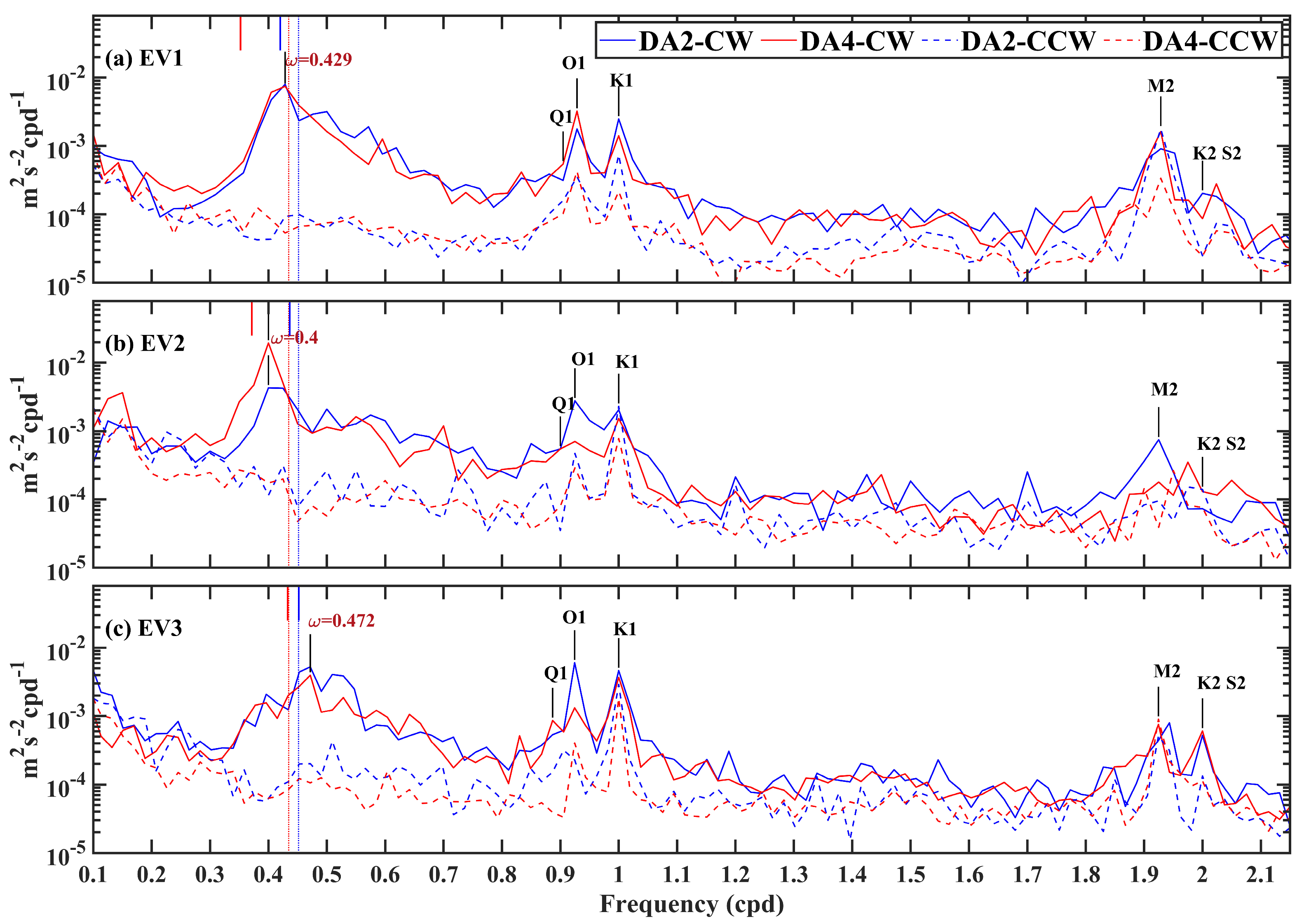
2.2. Velocity Rotary Spectra

Rotary spectra are used to describe the rotation components of current motions at various frequencies [46]. For any horizontal current, where u is zonal velocity and v is meridional velocity,

$$U\left(t\right)=u\left(t\right)+iv\left(\mathrm{t}\right)$$

(1)

Perform the Fourier transform of $U\left(t\right)$.

$$\sum _{k=0}^N{A}_{(1,k)}cos\left({\omega }_{k}t\right)+A_{(2,k)}sin\left({\omega }_{k}t\right)+i\times \sum _{k=0}^N{B}_{(1,k)}cos\left({\omega }_{k}t\right)+B_{(2,k)}sin\left({\omega }_{k}t\right)$$

(2)

where ${\omega }_{\mathrm{k}}=2\pi \mathrm{k}/\mathrm{T}$ (T is the length of the dataset) is the angular frequency, A and B are the amplitudes of u and v at k. The current ellipse is the sum of the of clockwise (−) and anticlockwise (+) components. The kinetic energy spectra or total rotary amplitude spectra is defined as [39,46]:

$$P_{KE}\left(\mathsf{\omega }\right)=P_{-}\left(\mathsf{\omega }\right)+P_{+}\left(\mathsf{\omega }\right)$$

(3)

where P₊(ω) is the anti-clockwise rotary spectrum, where $W_k^{+}$ and $W_k^{-}$ denote the amplitudes of Fourier transform at ${\omega }_k$:

$$P_{+}\left(\mathsf{\omega }\right)={\left(W_k^{+}\right)}^2/T$$

(4)

where P₋(ω) is the anti-clockwise rotary spectrum:

$$P_{-}\left(\mathsf{\omega }\right)={\left(W_k^{-}\right)}^2/T$$

(5)

Figure 3a,b illustrates the P_KE of moorings DA2 and DA4 throughout the observation period. It is evident that the diurnal tidal components (O₁ and K₁) have a pronounced impact on DA2 which is denoted by the black vertical dashed lines, particularly in the shallow to mid-depth range (100–300 m). DA4 exhibits a stronger tidal response. Both moorings display broadband characteristics in the near-inertial frequency band. For DA2, the peak in the near-inertial band which is delineated by the dotted gray line is primarily concentrated in the upper 250 m, while for DA4, it occurs at greater depths (300–650 m), accompanied by a distinct redshifted spectral peak. Additionally, peaks corresponding to the semidiurnal tidal components (M₂ and S₂) are observed, though their intensities are relatively weaker. Therefore, our study focuses on diurnal ITs and NIWs to describe their spatiotemporal variability and the underlying driving mechanisms.

2.3. Calculation of Coherent and Incoherent Motions

A fourth-order Butterworth filter is applied to the time series of the residual currents at each depth to extract the diurnal ITs’ currents (u and v). The cut-off frequencies of the diurnal bands are set to [0.79, 1.15] cpd (1 cpd = 2π/86,400/s).

Then, we separate the purely deterministic current signal from the 13−month ADCP record by applying a sharp harmonic filter [42,47]. Define the deterministic currents u₀ as the sum of a series of primary tidal currents at harmonic constituent frequencies:

$$u_0=\sum U_n\mathit{cos}\left({\psi }_n+{\omega }_{n}t\right)$$

(6)

where ω_n = Q₁, O₁, P₁, and K₁ are the dominant components in diurnal tidal motions in the SCS [48], and U_n are the amplitudes, ${\mathsf{\psi }}_{\mathrm{n}}$ are the phases, and similar definitions apply for v. In this way, we can extract the parts of the ITs which are coherent with the local barotropic tide phase. The residual currents containing incoherent ITs are defined as follows:

$$u^{\prime }=u-u_0$$

(7)

3. Results

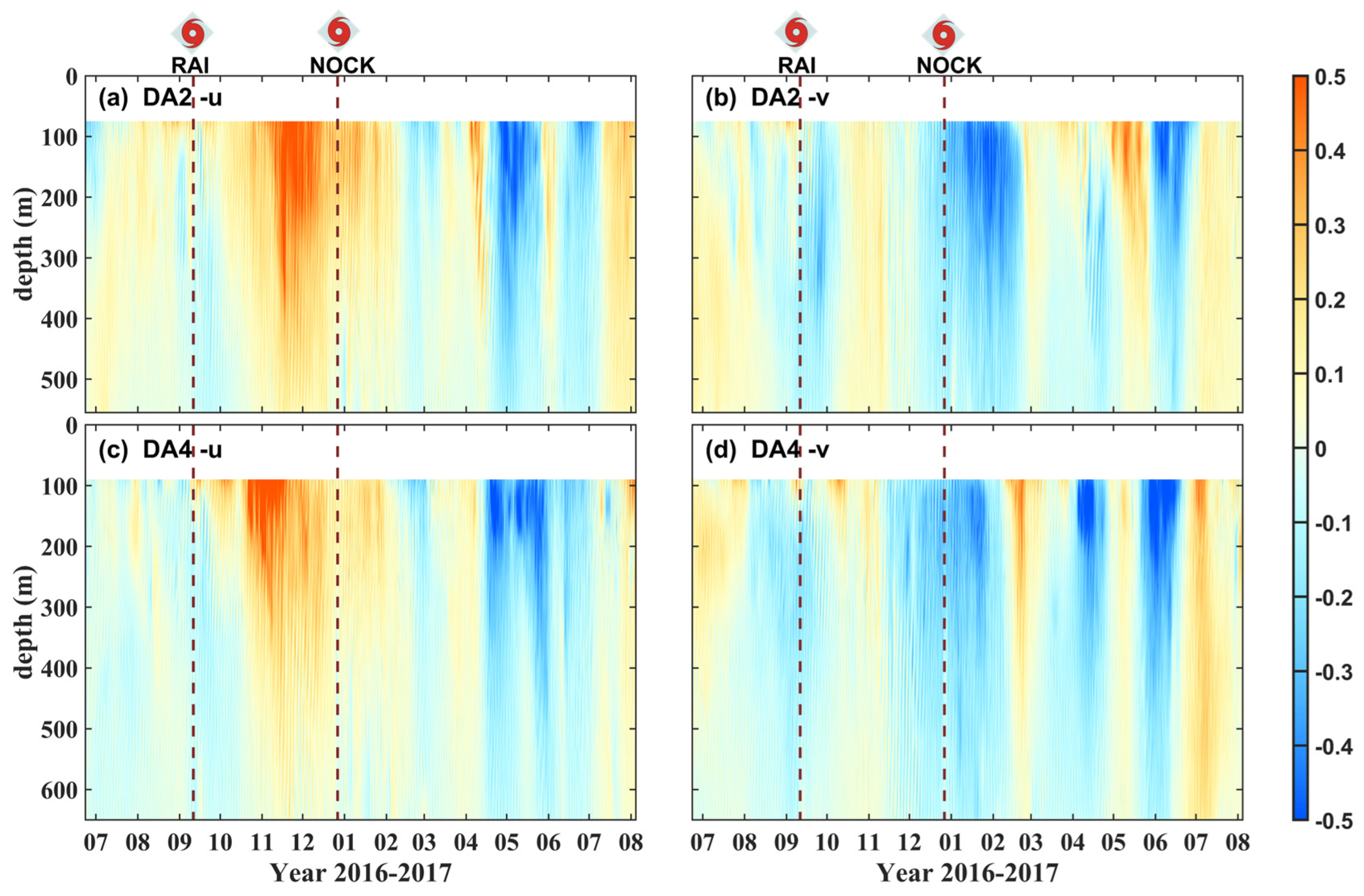
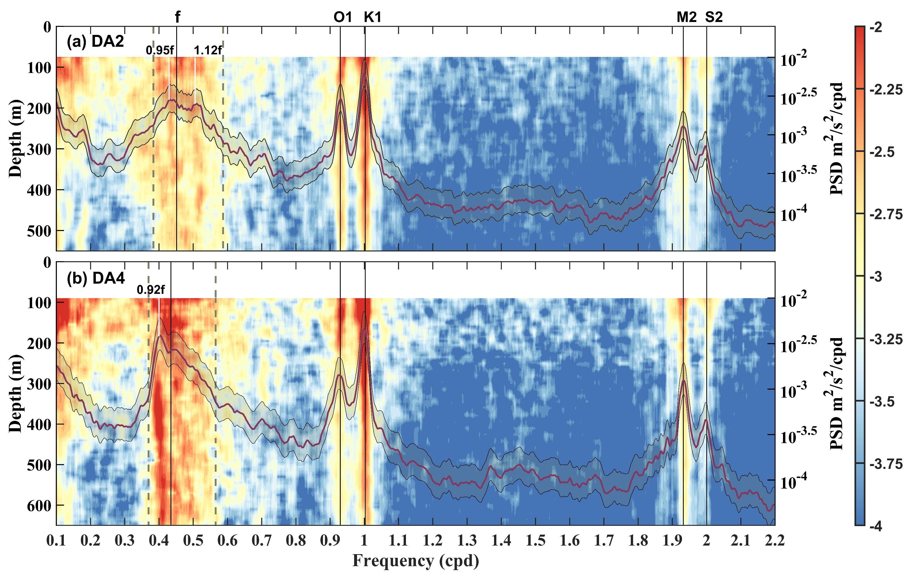
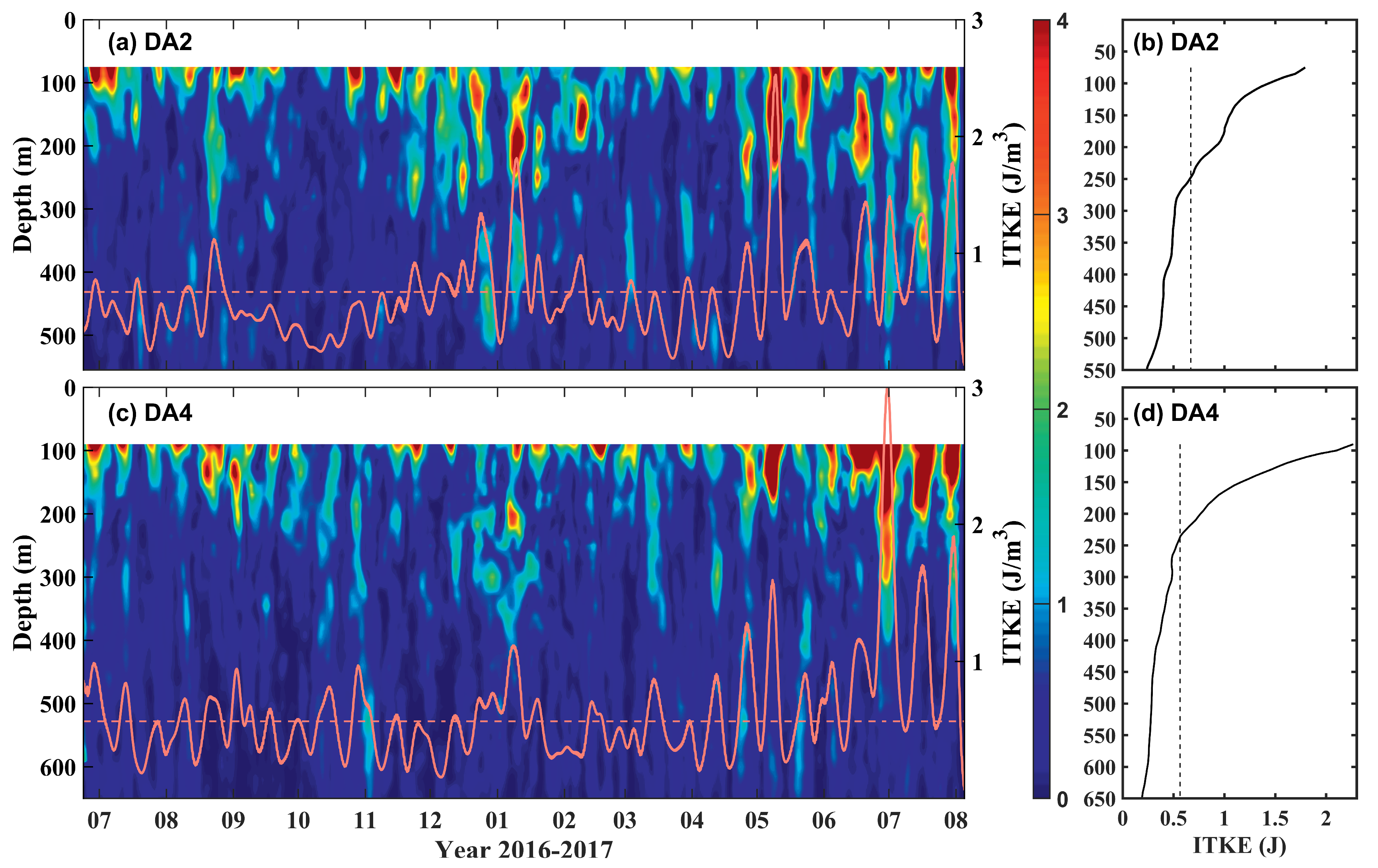
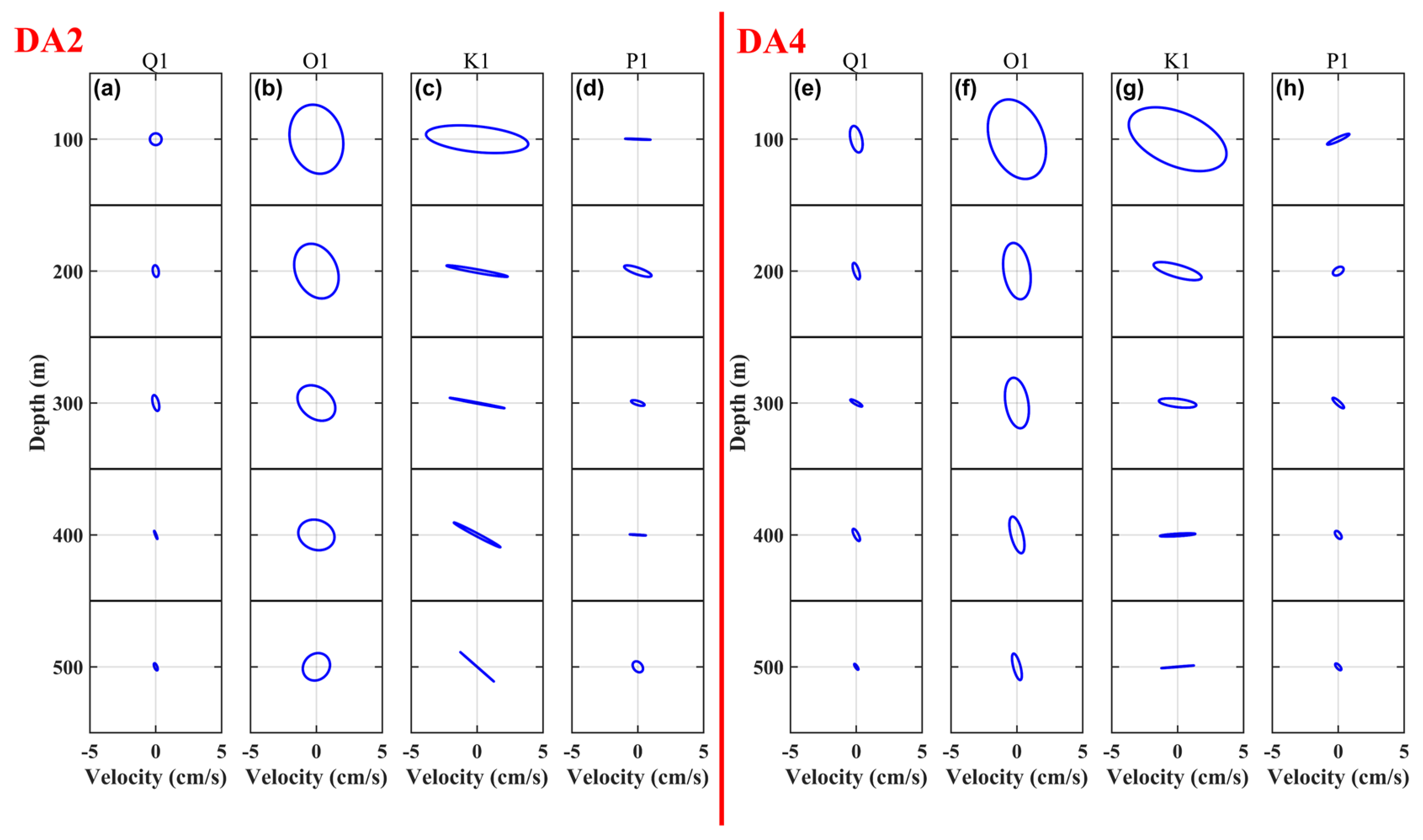
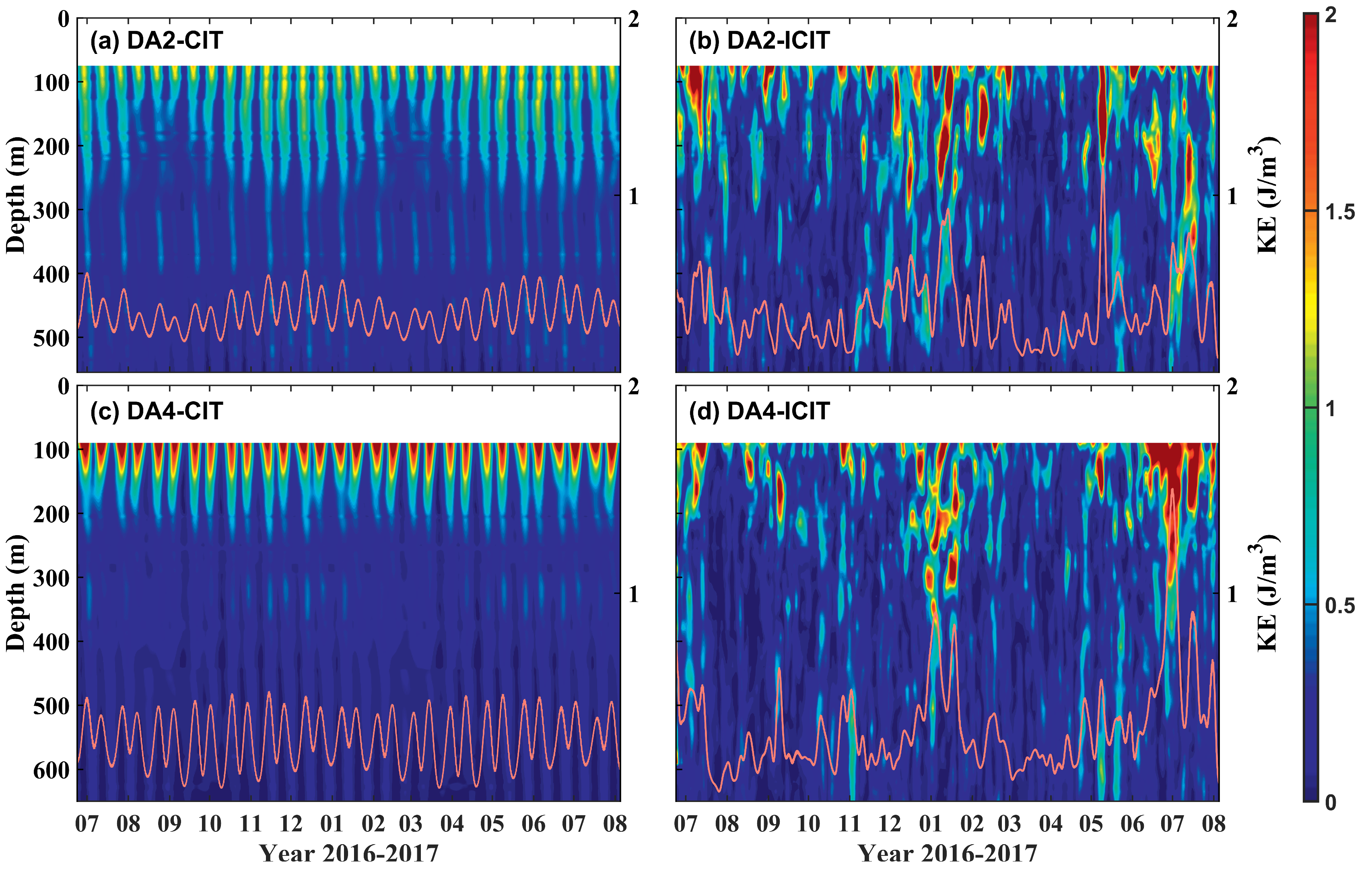
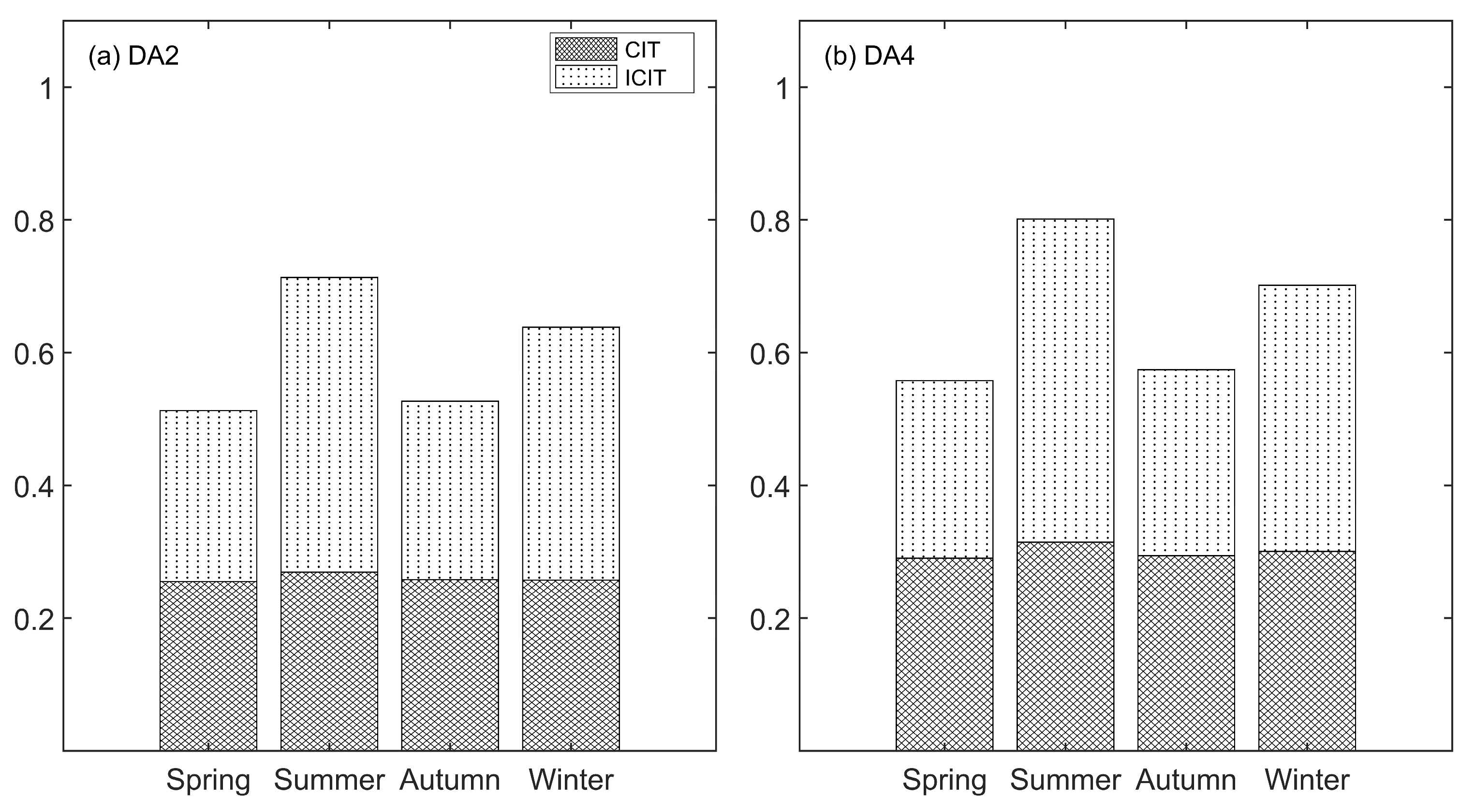
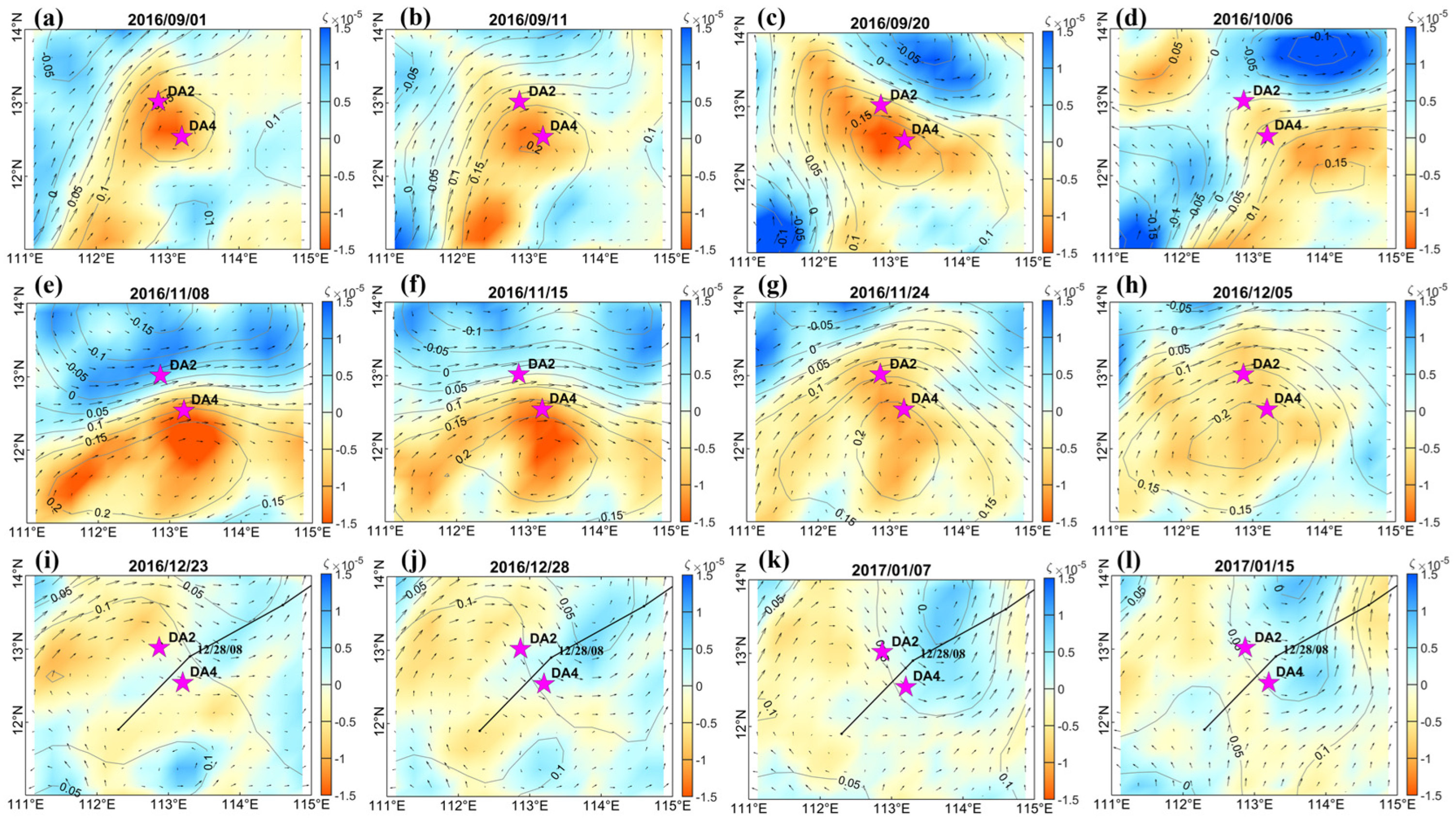
3.1. Evolution of Diurnal Internal Tides

This section analyses the spatial and temporal distributions of diurnal ITs. Based on ADCP observations and using an average seawater density of 1024 ${\mathrm{k}\mathrm{g}/\mathrm{m}}^3$, the depth and time-averaged horizontal kinetic energy (KE) of diurnal ITs is calculated as 0.56 ${\mathrm{J}/\mathrm{m}}^3$ (0.67 ${\mathrm{J}/\mathrm{m}}^3$) for DA2 (DA4). As shown in Figure 4, the time-varying characteristics of diurnal KE at the two moorings are synchronized, displaying a clear cycle of spring–neap oscillations with a period of approximately 14 days, which is primarily caused by the interfering effect of the K₁ and O₁ ITs. Additionally, the diurnal KE at both moorings is enhanced during May to July 2016 and December 2016 to February 2017, exhibiting a semiannual modulation due to the interference of K₁ and P₁ internal tides. The strongest diurnal KE during the observation period occurred around 10 May 2017 for DA2 and early July 2017 for DA4. In terms of vertical distribution, the KE at both sites is primarily concentrated at depths shallower than 250 m, with a rapid decrease below this depth, indicating the dominance of low-mode ITs propagating from the far field. The similarity in the spatial and temporal distributions of diurnal KE at the two moorings suggests that they may originate from the same generation site.

To further investigate the vertical distribution and horizontal propagation direction of the diurnal ITs in the southern SCS, the S_Tide toolbox is employed for standard harmonic analysis [49] to obtain the vertical distribution of tidal current ellipses for each constituent. As shown in Figure 5, the local baroclinic phase-locked tidal currents are stronger than the barotropic tidal currents, with the O₁ and K₁ constituents being comparable and significantly larger than that of Q₁ and P₁. Notably, O₁ exhibits characteristics of rotary tidal currents, whereas K₁ tends to display rectilinear tidal currents, especially at depths below 200 m. In terms of baroclinic current velocity, the maximum K₁ tidal current reaches 2.08 ${\mathrm{c}\mathrm{m}\mathrm{s}}^{-1}$ for DA2 and 1.86${\mathrm{c}\mathrm{m}\mathrm{s}}^{-1}$ for DA4, while the maximum O₁ tidal current reaches 2.25 ${\mathrm{c}\mathrm{m}\mathrm{s}}^{-1}$ for DA2 and 2.28 ${\mathrm{c}\mathrm{m}\mathrm{s}}^{-1}$ for DA4. All tidal constituents show a monotonic decrease with increasing depth, exhibiting characteristics of mode-1. The propagation direction of the O₁ constituent exhibits a dominant north–south component compared to the east–west component, whereas the K₁ constituent shows a stronger east–west component. For the K₁ constituent, the north–south component is stronger at DA4 than at DA2. Both constituents exhibit a monotonic decrease in intensity with depth, reflecting the characteristics of low-mode internal tides.

Despite the presence of a spring–neap cycle, strong irregularity in the diurnal ITs is still observed (Figure 4); both DA2 and DA4 exhibit intermittent peaks at depths shallower than 250 m. Considering that the propagation of diurnal ITs is susceptible to being modulated by multi-scale dynamic processes such as eddies and circulations, the coherent and incoherent components of diurnal ITs are separately decomposed (Figure 6). For the coherent ITs, the KE at DA2 is primarily concentrated at depths shallower than 300 m and gradually decreases with increasing depth. During spring tides, weaker peaks are also observed in deeper layers around 400 m. Temporally, the intensity of coherent ITs exhibits a distinct semiannual cycle. The KE of the coherent component in the upper layer of DA4 is stronger than that of DA2, but its contour line of KE = 0.6 ${\mathrm{J}\mathrm{m}}^{-3}$ is shallower. The enhanced KE at DA4 is primarily concentrated within the upper 180 m. This results in the depth-averaged energy at DA2 (0.34 ${\mathrm{J}\mathrm{m}}^{-3}$) being higher than that at DA4 (0.30 ${\mathrm{J}\mathrm{m}}^{-3}$). For incoherent diurnal ITs, the incoherent component accounts for 54% and 56% of the total KE at DA2 and DA4, respectively, which is lower compared to the results from the northern SCS [19]. This finding is consistent with the conclusions of Liu et al. [42], and the high incoherence can be attributed to energy dissipation during the propagation [15]. The diurnal KE is dominated by the incoherent component which contributes to most of the strong internal tide events.

We further investigate the seasonal variation in diurnal KE. In this study, the seasonal division is defined as follows: The seasonal analysis of diurnal KE reveals a “two-strong, two-weak” variation pattern, with significantly stronger diurnal internal tidal kinetic energy in summer and winter compared to autumn and spring, leading to a semiannual cycle of variation (Figure 7). Although the coherent and incoherent components are comparable, the seasonal-scale variation is primarily contributed by incoherent ITs, accounting for 99.3% of the variance at DA2 and 99.5% at DA4, while the seasonal variation in coherent ITs at the two mooring sites is not significant.

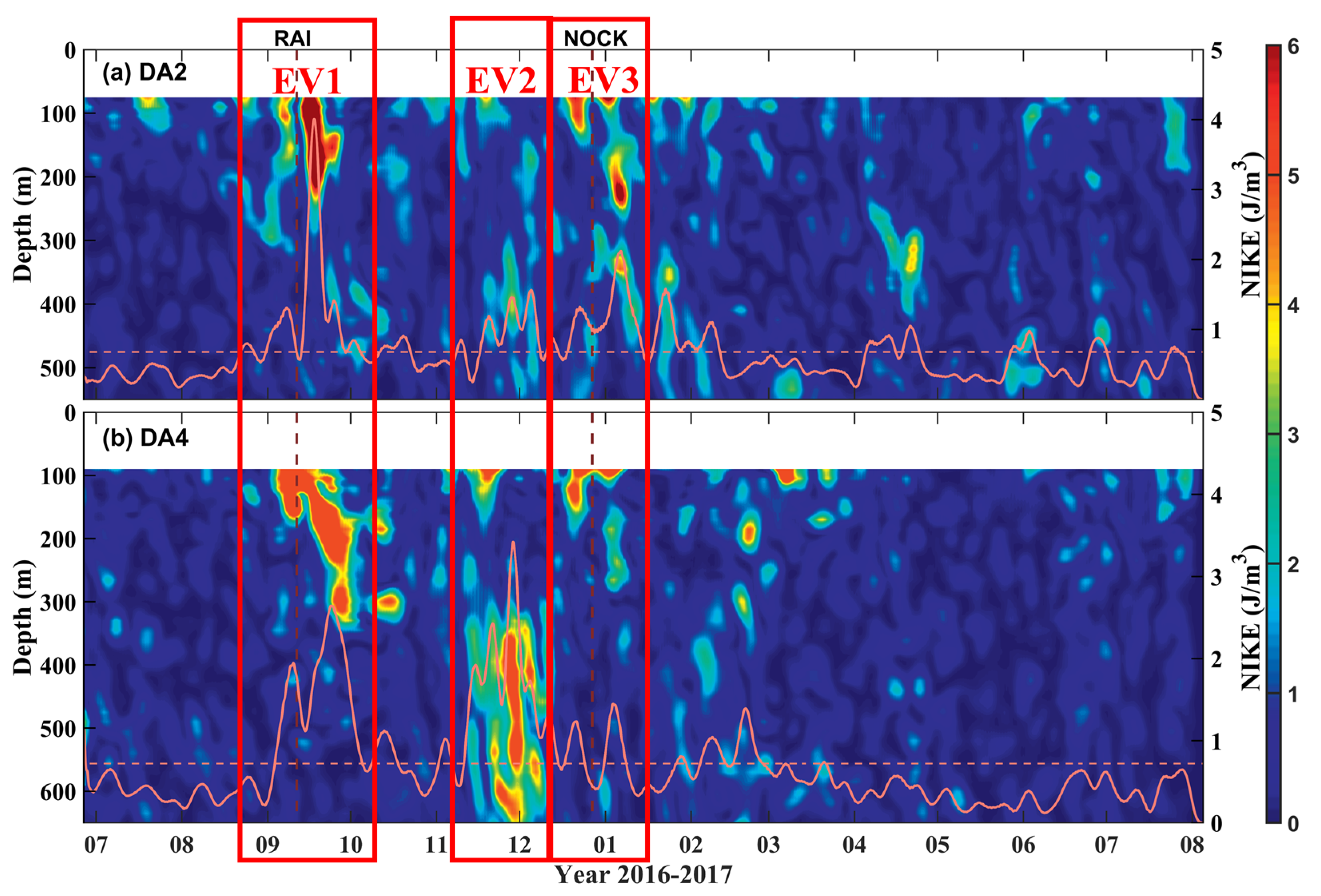
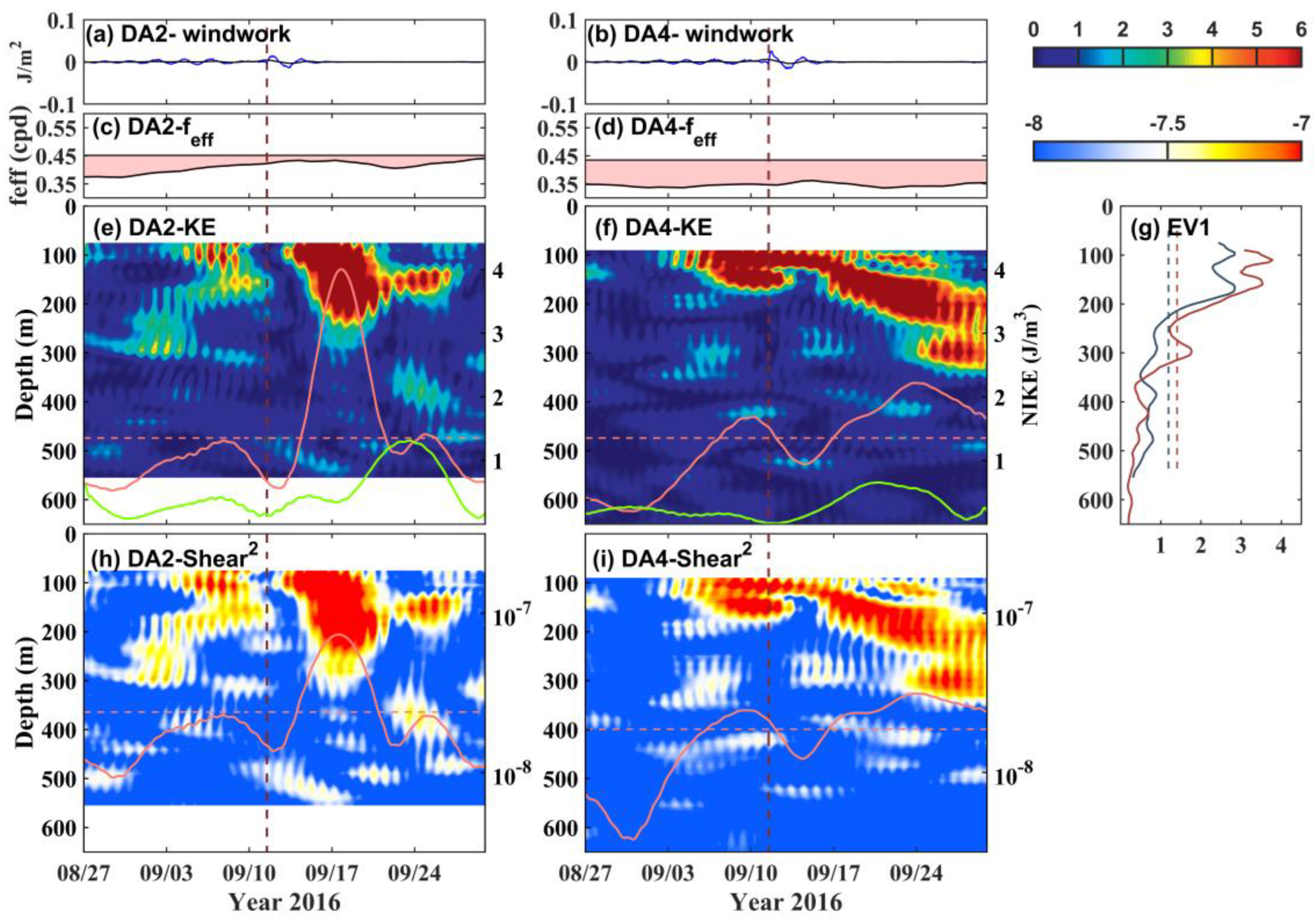
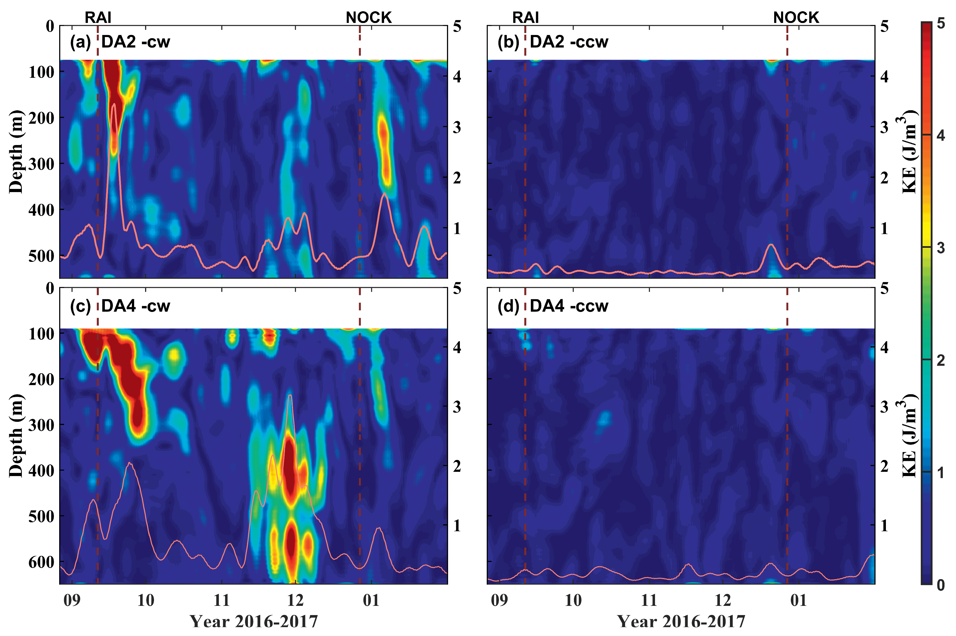
3.2. Near-Inertial Waves Induced by Tropical Cyclone RAI (Event 1)

Figure 8 shows the depth–time distribution of near-inertial KE during the observation period at moorings DA2 and DA4, the purple horizontal dashed line indicates the average value of this time series, and the brown dotted line indicates the latest time from RAI and NOCK to the station. Near-inertial KE exhibits strong temporal intermittency, with concentrations from September 2016 to March 2017, aligning with the timing of tropical cyclones in the SCS. During the passage of two TCs, intense NIWs are generated at the two mooring sites. However, due to the differences in the characteristics of the TCs, distances between TC centers and the moorings, and local conditions, the characteristics of NIWs at the two moorings also vary, which will be discussed in detail later. In addition to the TC-induced NIWs, though no TCs were reported close to the mooring sites, an unexpected NIW burst event was observed between November and December 2016. In this study, the near-inertial events induced by RAI and NOCK are referred to as event 1 (1 September to 6 October) and event 3 (15 December to 15 January), respectively. The NIW burst event observed from November to December is referred to as event 2 (5 November to 15 December).

Four days prior to the passage of RAI, a relatively weak peak in near-inertial KE was observed in the upper 300 m at DA2, exceeding the mean level by only 5%. Approximately 30 h after the TC’s passage, surface the near-inertial KE rapidly intensified, reaching a maximum value of 19.55 ${\mathrm{J}\mathrm{m}}^{-3}$. Over the next two inertial periods (approximately five days), this intensification propagated to a depth of 300 m, resulting in an increase of over 300% in depth-averaged near-inertial KE within the mooring. The distribution of near-inertial shear was similar as that of near-inertial KE, with significant enhancement observed at a depth of 250 m following RAI’s passage (Figure 9e). This NIW event is the strongest at DA2, with the NIW induced by TC RAI persisting for approximately 14 days. In contrast, the near-inertial KE at DA4 appeared to be more continuous. Near-inertial KE values exceeding 5 ${\mathrm{J}/\mathrm{m}}^3$ are more widely distributed and exhibit few interruptions in the upper layers in the depth–time plot (the purple solid line in Figure 9f). Beginning about one week before RAI, prominent near-inertial oscillations were observed in the shallow region above 170 m at DA4, with the magnitude of near-inertial KE being approximately 1.4 times the mean value. Following the TC’s passage, near-inertial KE was intensified rapidly above 130 m, reaching a maximum value of 18.82 ${\mathrm{J}\mathrm{m}}^{-3}$. However, within the first four days after RAI, no further downward propagation occurred, and the shear remained confined above 130 m (Figure 9h,i). It was not until 16 September that the near-inertial KE began to propagate deeper, eventually reaching a depth of 330 m by 28 September. After the TC’s passage, enhanced NIWs at DA4 persisted for 22 days.

Comparing the near-inertial responses at the two moorings during event 1, DA2 exhibits a stronger increase in near-inertial KE following RAI’s passage, likely due to its closer distance to the cyclone. However, the post tropical cyclone near-inertial KE at DA4 persisted for approximately 10 days longer than at DA2. In terms of the vertical near-inertial KE distribution, the values at DA4 decayed below the mean value below 320 m, with several peaks observed at 100 m, 150 m, and 300 m. In contrast, the propagation depth of near-inertial KE at DA2 was shallower, reaching only 220 m, with peaks at 100 m and 170 m. In summary, while RAI induced stronger NIWs in the upper ocean at DA2, the NIWs observed at DA4 lasted longer and propagated to greater depths (Figure 9g).

As shown in Figure 9c,d, both mooring systems are influenced by a negative background vorticity field during event 1. Figure 10a,d illustrate that event 1 coincides with the weakening phase of a jet stream off the eastern coast of the Vietnam Peninsula. On 1 September, the axis of the jet stream shifted from east to northeast within the range of 109° E–113° E, with positive vorticity dominating the northwest side and negative vorticity on the southeast side. As the jet stream axis gradually weakened, the anticyclonic eddy expanded northwestward with increasing intensity. Simultaneously, the cyclonic eddy northeast of the anticyclonic eddy also developed, forming a mesoscale eddy pair near DA2 by 20 September. By 25 September, the anticyclonic eddy reached its maximum intensity before beginning to weaken. Throughout the event 1 period, both DA2 and DA4 were located within the influence of the anticyclonic eddies; however, the negative vorticity at DA4 consistently exceeded that at DA2. As previously analyzed, TC RAI passed closer to DA2, leading to the higher near-inertial KE peaks recorded at this site. Nevertheless, the trapping effect of the anticyclonic eddies at DA4 contributed to a greater propagation depth and a longer duration of NIWs compared to DA2.

Rotary spectral results indicate that during the passage of RAI, the near-inertial frequency peaks at DA2 and DA4 are significantly enhanced, as shown in Figure 11, with the clockwise component dominating and surpassing the energy levels of $D_1$ITs and $D_2$ITs internal tides (Figure 11a). Both moorings display a pronounced redshift in their near-inertial frequency peaks. At DA2, three distinct peaks are identified, with the largest and second-largest peaks exhibiting clear redshifts at 0.95f and 0.89f, respectively. At DA4, two peaks are observed within the near-inertial frequency band, with the largest peak occurring at 0.98f, matching the frequency of the largest peak at DA2, while the second-largest peak is identified at 0.93f. The redshifted peaks at DA2 and DA4 indicate the existence of an anticyclonic eddy, which lowers the near-inertial band and tends to trap NIWs.

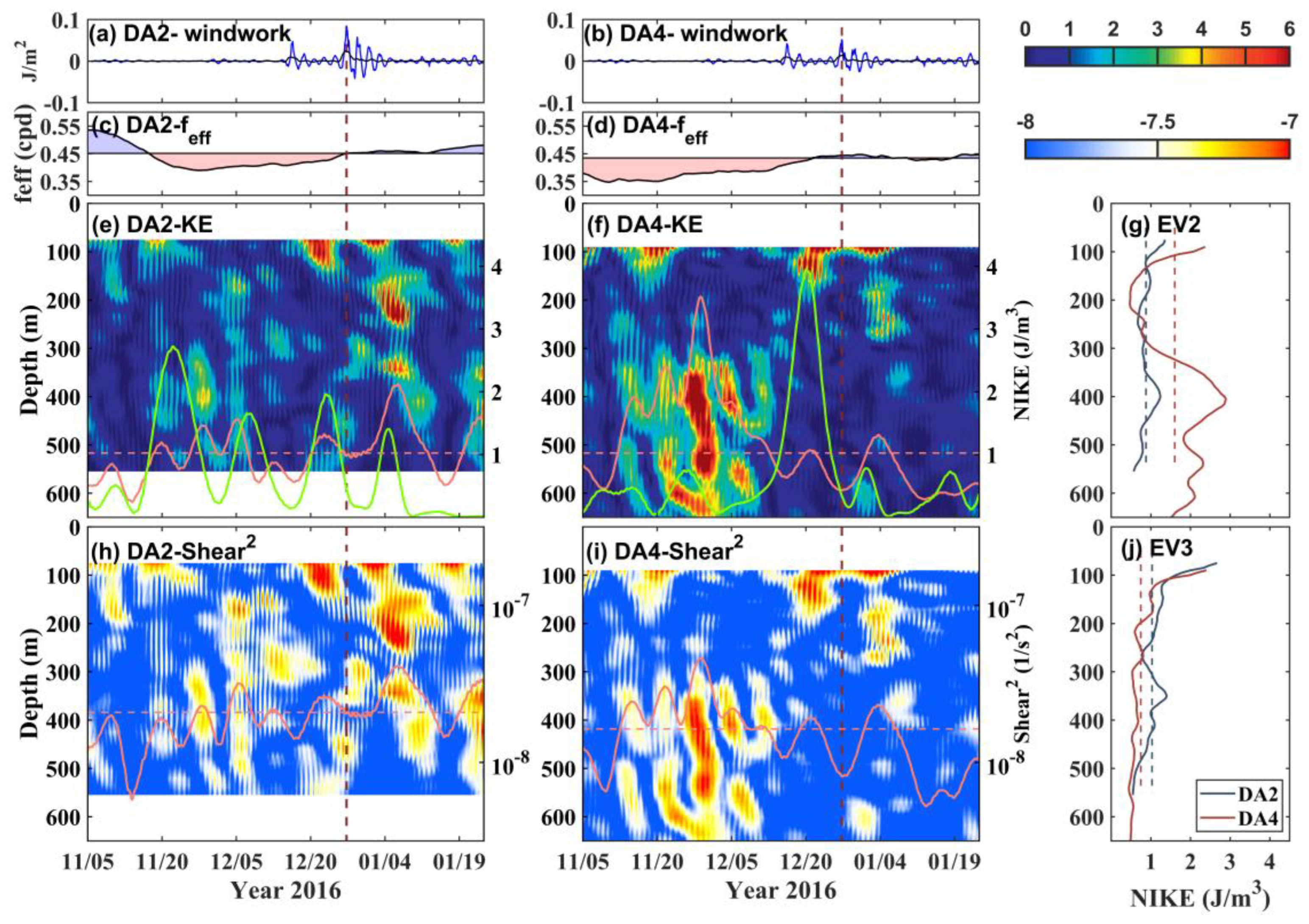
3.3. Near-Inertial Waves from November to December (Event 2)

During event 2, no TC passed near either mooring system; the peak in wind work observed from 15 to 20 December was induced by changes in the monsoon. At DA2, three step-like increases in near-inertial KE are observed on 20 November, 28 November, and 5 December, with peaks exceeding the average value by 70% (Figure 12e). However, the intensity of event 2 is significantly weaker compared to event 1 and event 3 induced by the two TCs. Notably, DA4 records its strongest NIW event during this period (Figure 12f), surpassing event 1 and event 3 in terms of propagation depth and duration, and the magnitudes of near-inertial KE at DA4 are greater than the average level from 12 November to 12 December and are significantly enhanced under 350 m. Similarly, three step-like near-inertial KE peaks are observed at DA4 on 13 November, 22 November, and 30 December, with the strongest peak reaching approximately 2.5 times the average value, occurring about five days earlier than the corresponding peaks at DA2. In terms of vertical distribution, the energy at DA2 is primarily concentrated between 360 m and 460 m. However, at DA4, near-inertial KE is distributed between 300 and 650 m, with the strongest NIW of the year at 1000 m occurring 25 days after the maximum appears in the upper layer (the green solid line in Figure 12g).

Due to the proximity of the mooring systems to the critical latitude for the parametric subharmonic instability (PSI) of the diurnal ITs [40,50], we decompose the near-inertial KE into clockwise and counterclockwise components to rule out PSI as a primary mechanism. As shown in Figure 12, throughout the observation period, downward-propagating components dominate the near-inertial waves at both mooring systems. During event 2, the downward-propagating near-inertial KE at DA2 and DA4 is more than an order of magnitude stronger than the upward-propagating component. This contrasts with the characteristics of waves generated by the PSI mechanism, where the ratio of counterclockwise to clockwise components is typically comparable. Although previous study [3] suggests that PSI could occur up to 20 km beyond the critical latitude under the modulation of relative vorticity, our observations during event 2 seem to suggest a different scenario. While the background field is characterized by negative vorticity, the downward-dominant characteristics of near-inertial KE at both moorings imply that PSI may not be the primary mechanism responsible for the enhancement of near-inertial KE.

Therefore, the contribution of lateral near-inertial KE propagation to this event is considered. At the early stage of event 2, a west-to-east extending jet stream is located between DA2 and DA4, with a cyclonic eddy region to the north of the axis and an anticyclonic eddy region to the south (Figure 10e–h). The two moorings are positioned at the edges of the cyclonic eddy and anticyclonic eddy, respectively. Subsequently, the anticyclonic eddy on the southern side gradually migrates northward and takes control of DA2 by 18 November. After the background field of DA2 transitions from the cyclonic eddy to the anticyclonic eddy, the near-inertial KE above 500 m rapidly intensifies. Subsequently, the anticyclonic eddy continues to expand its size, with its vorticity gradually weakening. Different from DA2, DA4 remains closer to the center of the anticyclonic eddy, where the negative vorticity is stronger, leading to the lower f_eff. Due to the “inertial chimney” effect of the anticyclonic eddy, a more intense near-inertial KE which propagates deeper is observed at DA4 (Figure 12). Significantly enhanced near-inertial KE is observed at DA4 between 300 and 650 m. Meanwhile, 25 days after the peak observed in the upper layers at DA4 on November 25th, the current meter at a depth of 1000 m also detects significantly enhanced NIWs. Considering the vertical propagation speed of near-inertial internal waves (30 $\mathrm{m}/\mathrm{d}\mathrm{a}\mathrm{y}$), we conclude that the NIWs in the upper layers propagate to depths greater than 1000 m under the trapping effect of anticyclonic eddies. The time-averaged near-inertial KE at DA4 is nearly twice that of DA2, which is directly proportional to the distance from the center of anticyclonic eddy. This further indicates that the anticyclonic eddy plays a role in regulating the lateral and vertical propagation of NIWs. Compared to event 1, although both events are influenced by negative background vorticity, event 2 is characterized by a larger anticyclonic eddy with a longer duration. This enables the anticyclonic eddy to trap near-inertial KE over a broader area and provides a longer amount of time for near-inertial KE to propagate into the deep ocean.

During event 2, the clockwise spectra (Figure 11b) at DA4 are dominated by near-inertial frequencies, with the near-inertial peak nearly an order of magnitude higher than the spectral values at the O₁ and K₁ frequencies. In contrast, the near-inertial KE at DA2 is weaker than the diurnal KE. The significant near-inertial peak is dominated by the clockwise component which has clear redshifts (0.886 f for DA2 and 0.92 f for DA4), while the counterclockwise spectra in the near-inertial band remain weak. Additionally, during event 3, DA2 also exhibits a peak in the clockwise spectrum at 0.5 cpd.

3.4. Near-Inertial Waves Induced by Tropical Cyclone NOCK (Event 3)

During event 3, DA2, located on the right side of the tropical cyclone’s path, observes a near-inertial KE peak five days before NOCK’s passage, reaching 1.1 times the mean value and propagating to 150 m (Figure 12). On the first day after NOCK, the near-inertial KE intensifies above 100 m and persists for six days without further downward propagation. By the seventh day after NOCK, downward-propagating near-inertial KE appears at depths of 200–300 m and lasts for about seven days. During this period, the depth-averaged near-inertial KE exceeds the mean value by 80%. Based on the distribution of near-inertial KE, the energy below 200 m is not directly transmitted from the upper 100 m (Figure 12e). At DA4, located on the left side of the TC’s path, the temporal and spatial variations in near-inertial KE are generally similar as those at DA2, with the post-TC near-inertial KE peak occurring slightly earlier than at DA2, likely due to DA4’s closer proximity to NOCK’s center. However, the near-inertial KE at DA4 is weaker and has a shorter duration, which is consistent with theoretical expectations of enhanced near-inertial waves on the left side of a TC’s path [8]. In terms of vertical distribution, the energy at DA2 is primarily concentrated above 230 m, with an additional peak observed near 350 m. At DA4, the energy is mainly concentrated above 200 m, with only a weaker peak in the 250–300 m depth range.

The vorticity field during event 3 is shown in Figure 10e–h, which reveal that both mooring systems are initially under the influence of weak negative vorticity. Meanwhile, a region of positive vorticity located northeast of the moorings gradually expands southwestward. By the time of NOCK’s passage, the areas around both moorings are essentially in a vorticity-neutral state. After the tropical cyclone passed, the cyclonic eddy northeast of the moorings intensified, reaching its peak strength on 5–6 January, before starting to weaken. During this time, both moorings were situated on the edges of the cyclonic eddy. During event 3, surface-enhanced near-inertial KE was observed before the arrival of NOCK. The background field was filled with negative vorticity conditions, which enabled NIWs to propagate to greater depths compared to the post-TC period. In comparison to event 1, although NOCK was stronger than RAI, and thus the wind-induced near-inertial energy input was also higher for NOCK, the near-inertial KE observed during event 1 at both moorings was significantly greater in intensity and propagation depth.

During event 3, the rotary spectra indicate that the near-inertial band energy at both moorings is enhanced during NOCK’s passage (Figure 11c). However, the overall intensity is weaker and does not exceed the peak energy of the diurnal O₁ frequency. At DA2, the peaks exhibit a blue shift, appearing at 1.045, 1.00, and 1.169f. At DA4, the near-inertial peaks appear at 1.086 f and 0.996 f, with the maximum peak frequency matching that observed at DA2.

4. Discussion

In this study, the variability of diurnal internal tides and near-inertial waves are investigated by two moorings located in the southern South China Sea. During the observation period, both settings exhibited dominant diurnal ITs and NIWs in the internal wave frequency band, and weaker peaks were also observed for the semidiurnal tides (Figure 3). The averaged diurnal KE between 100 and 500 m is 0.56 ${\mathrm{J}/\mathrm{m}}^3$ for DA2 and 0.67 ${\mathrm{J}/\mathrm{m}}^3$ for DA4, with the O₁ and K₁ tidal constituents being dominant. Under the interference of the two tidal constituents, diurnal KE exhibits a clear spring–neap modulation cycle (Figure 4). The semiannual cycle of diurnal KE (with stronger values in summer and winter than in spring and autumn) is caused by the interference between the P₁ and K₁ tidal constituents. The irregularity of diurnal KE over time is caused by incoherent ITs, which control several strong diurnal IT events. Vertically, diurnal KE is concentrated more shallowly than 250 m and rapidly decreases below the average as depth increases which suggests that the majority of low-mode internal tides propagate from the far field (Figure 4b,d).

Three concentrated NIW events were captured (Figure 8). The velocity decomposition results indicate that the downward component at both DA2 and DA4 is much larger than the upward component, suggesting that wind-driven NIWs are the primary source of NIWs in this region (Figure 13). Event 1 is associated with TC RAI, which is the closest to the stations on 12 September. During event 1, near-inertial KE reached a maximum of 19.55 J m⁻³ for DA2 and 18.82 J m⁻³ for DA4 at 100 m and 110 m, respectively, and gradually decreased with depth. For DA2, event 1 was the strongest event observed during its monitoring period (Figure 9). The NIWs generated by RAI propagated to a depth of 220 m, and the depth-averaged near-inertial KE remained above the average value for 13 days before decreasing below the average. For DA4, the energy of event 1 was transmitted to a depth of 320 m and lasted for 22 days. Event 3 was associated with TC NOCK, which passed the mooring stations on December 28. The two moorings were located on different sides of the best path of NOCK (Figure 1). DA2 was located on the right side of the path, and observed a stronger near-inertial KE than DA4, which was consistent with the theoretical expectation of enhanced near-inertial waves on the right side of the path. Although the near-inertial energy input into the ocean by NOCK was much stronger than that of RAI, the near-inertial KE intensity observed during event 3 was significantly weaker than that of event 1, and the duration was also shorter, lasting around 10 days. Additionally, the NIWs observed by both moorings at shallower than 100 m did not propagate downward. In the depth–time distribution of near-inertial KE and the near-inertial KE observed at depths of 200–300 m on the seventh day after the typhoon’s passage were not continuous with the near-inertial KE that appeared in the upper 100 m layer after NOCK.

We thought that the modulation effect of cyclonic eddies and anticyclonic eddies influenced the horizontal and vertical propagation of NIWs. During event 1, the stronger negative vorticity at DA4 allowed the NIWs to propagate more deeply, and the strongest near-inertial event was observed at DA4 during event 3 (with a peak also occurring at a depth of 1000 m). Through rotation spectrum analysis, it was found that during the anticyclonic eddies-controlled period, the maximum value of the near-inertial frequency band on the rotation spectrum redshifted relative to f, with the redshift becoming more pronounced as the anticyclonic eddies intensified (Figure 11). In contrast, under conditions of no eddy or cyclonic eddy control, the peak frequency of the NIWs shifted blueward. Based on the above analysis, mesoscale eddy processes have a significant impact on the propagation and spatio-temporal variation characteristics of NIWs. Mesoscale eddies modulate the frequency of locally generated NIWs by altering the effective inertial frequency. Anticyclonic eddies promote the downward transfer of near-inertial energy through the “inertial chimney”, while cyclonic eddies suppress the downward propagation of NIWs.

The findings of this study have significant practical implications for oceanographic research and environmental management. First, understanding the behavior of ITs and NIWs is crucial for predicting the ocean mixing and energy distribution in the southern SCS, particularly in deep-ocean regions. This would make existing climate models closer to the real ocean when a tropical cyclone path goes through this region, or during spring tide events, thereby improving predictions of future climate change, especially in the context of increasingly intense global warming and the increase in extreme disasters. Finally, the results could be applied in optimizing the deployment of oceanographic instrumentation for monitoring internal waves. However, several limitations should be noted: A simplified slab model was used to calculate wind-driven near-inertial energy, which may not fully capture the complexity of wind–wave interactions, especially in regions dominated by mesoscale eddies and complex stratification. Future research could adopt advanced numerical models that integrate 3D ocean dynamics and higher-resolution wind field data to improve the accuracy of near-inertial energy predictions and enhance the understanding of wave propagation processes. This study also highlights the need for further exploration of the modulation of ITs and NIWs by mesoscale eddies. Future investigations could delve deeper into the interactions between eddies and waves, particularly considering nonlinear interactions and their impact on deep-ocean mixing processes.

References

1. Mohapatra, S.C.; Guedes Soares, C. Boussinesq Model for Two-Fluid System with Surface- and Interfacial Tension. Appl. Ocean Res. 2024, 152, 104183. [Google Scholar] [CrossRef]
2. Alford, M.H.; Peacock, T.; MacKinnon, J.; Nash, J.D.; Buijsman, M.C.; Centurioni, L.R.; Chao, S.-Y.; Chang, M.-H.; Farmer, D.M.; Fringer, O.B.; et al. The formation and fate of internal waves in the South China Sea. Nature 2015, 521, 65–69. [Google Scholar] [CrossRef]
3. Moehlis, J.; Smith, S.L. Radiation of Mixed Layer Near-Inertial Oscillations into the Ocean Interior. J. Phys. Oceanogr. 2001, 31, 1550–1560. [Google Scholar] [CrossRef]
4. Jochum, M.; Briegleb, B.P.; Danabasoglu, G.; Large, W.G.; Norton, N.J.; Jayne, S.R.; Alford, M.H.; Bryan, F.O. The impact of oceanic near-inertial waves on climate. J. Clim. 2013, 26, 2833–2844. [Google Scholar] [CrossRef]
5. Munk, W.; Wunsch, C. Abyssal recipes II: Energetics of tidal and wind mixing. Deep. Sea Res. Part I Oceanogr. Res. Pap. 1998, 45, 1977–2010. [Google Scholar] [CrossRef]
6. Alford, M.H. Improved global maps and 54-year history of wind-work on ocean inertial motions. Geophys. Res. Lett. 2003, 30, 1424. [Google Scholar] [CrossRef]
7. St. Laurent, L.; Garrett, C. The role of internal tides in mixing the deep ocean. J. Phys. Oceanogr. 2002, 32, 2882–2899. [Google Scholar] [CrossRef]
8. Alford, M.H.; MacKinnon, J.A.; Simmons, H.L.; Nash, J.D. Near-inertial internal gravity waves in the ocean. Annu. Rev. Mar. Sci. 2016, 8, 95–123. [Google Scholar] [CrossRef] [PubMed]
9. Price, J.F. Upper ocean response to a hurricane. J. Phys. Oceanogr. 1981, 11, 153–175. [Google Scholar] [CrossRef]
10. Gill, A.E. On the behavior of internal waves in the wake of storms. J. Phys. Oceanogr. 1984, 14, 1129–1151. [Google Scholar] [CrossRef]
11. D’Asaro, E.A.; Sanford, T.B.; Niiler, P.P.; Terrill, E.J. Cold wake of Hurricane Frances. Geophys. Res. Lett. 2007, 34, L15609. [Google Scholar] [CrossRef]
12. Wunsch, C.; Ferrari, R. Vertical mixing, energy, and the general circulation of the oceans. Annu. Rev. Fluid Mech. 2004, 36, 281–314. [Google Scholar] [CrossRef]
13. Duda, T.F.; Rainville, L. Diurnal and semidiurnal internal tide energy flux at a continental slope in the South China Sea. J. Geophys. Res. Oceans 2008, 113, C03025. [Google Scholar] [CrossRef]
14. Chang, M.H.; Lien, R.C.; Tang, T.Y.; D’Asaro, E.A.; Yang, Y.J. Energy flux of nonlinear internal waves in northern South China Sea. Geophys. Res. Lett. 2006, 33, L03607. [Google Scholar] [CrossRef]
15. Alford, M.H.; Zhao, Z. Global patterns of low-mode internal wave propagation. Part I: Energy and energy flux. J. Phys. Oceanogr. 2007, 37, 1829–1848. [Google Scholar] [CrossRef]
16. Yang, Q.; Zhao, W.; Liang, X.; Tian, J. Three-Dimensional Distribution of Turbulent Mixing in the South China Sea. J. Phys. Oceanogr. 2016, 46, 769–788. [Google Scholar] [CrossRef]
17. Zhao, Z. Southward Internal Tides in the Northeastern South China Sea. J. Geophys. Res. Oceans 2020, 125, e2020JC016324. [Google Scholar] [CrossRef]
18. Zhao, Z. Internal tide radiation from the Luzon Strait. J. Geophys. Res. Oceans 2014, 119, 5434–5448. [Google Scholar] [CrossRef]
19. Liang, H. Observational Study on the Internal Tides and Near-Inertial Internal Waves in the Northern South China Sea. Ph.D. Thesis, Ocean University of China, Qingdao, China, 2015. [Google Scholar]
20. Xu, Z.; Liu, K.; Yin, B.; Zhao, Z.; Wang, Y.; Li, Q. Long-range propagation and associated variability of internal tides in the South China Sea. J. Geophys. Res. Oceans 2016, 121, 8268–8286. [Google Scholar] [CrossRef]
21. Zaron, E.D. Mapping the nonstationary internal tide with satellite altimetry. J. Geophys. Res. Oceans 2017, 122, 539–554. [Google Scholar] [CrossRef]
22. Song, P.; Chen, X. Investigation of the internal tides in the Northwest Pacific Ocean considering the background circulation and stratification. J. Phys. Oceanogr. 2020, 50, 3113–3133. [Google Scholar] [CrossRef]
23. Guan, S.; Jin, F.-F.; Tian, J.; Lin, I.-I.; Pun, I.-F.; Zhao, W.; Huthnance, J.; Xu, Z.; Cai, W.; Jing, Z.; et al. Ocean Internal Tides Suppress Tropical Cyclones in the South China Sea. Nat. Commun. 2024, 15, 3903. [Google Scholar] [CrossRef] [PubMed]
24. Liu, P.; Guan, S.; Lin, I.-I.; Huang, M.; Jin, F.; Wang, Q.; Lu, Z.; Zhao, W.; Tian, J. Response and Feedback of Mesoscale Eddies to Tropical Cyclones over the South China Sea. J. Geophys. Res. Atmos. 2025, 130, e2024JD041414. [Google Scholar] [CrossRef]
25. Wan, Y.-J.; Chen, G.-X.; Shu, Y.-Q.; Wang, Q.; Chen, R.-Y.; Wang, D.-X. Near-Inertial Oscillations Induced by Tropical Cyclones under the Background of South China Sea Winter Monsoon Surge: A Case Study of Mirinae (0921). J. Trop. Oceanogr. 2015, 34, 11–18. [Google Scholar] [CrossRef]
26. Chen, G.; Xue, H.; Wang, D.; Xie, Q. Observed near-inertial kinetic energy in the northwestern South China Sea. J. Geophys. Res. Oceans 2013, 118, 4965–4977. [Google Scholar] [CrossRef]
27. Li, J.; Xu, J.; Liu, J.; He, Y.; Chen, Z.; Cai, S. Correlation of near-inertial wind stress in typhoon and typhoon-induced oceanic near-inertial kinetic energy in the upper South China Sea. Atmosphere 2019, 10, 388. [Google Scholar] [CrossRef]
28. Liu, Q.; Cui, J.; Shang, X.; Xie, X.; Wu, X.; Gao, J.; Mei, H. Observation of Near-Inertial Internal Gravity Waves in the Southern South China Sea. Remote Sens. 2023, 15, 368. [Google Scholar] [CrossRef]
29. Mao, H.; Qi, Y.; Chen, Y.; Yu, J. Enhanced Mixing Induced by Near-Inertial Waves Inferred by Glider Observation in the Northern South China Sea. J. Mar. Sci. Eng. 2023, 11, 2141. [Google Scholar] [CrossRef]
30. Yang, B.; Hu, P.; Hou, Y. Observed Near-Inertial Waves in the Northern South China Sea. Remote Sens. 2021, 13, 3223. [Google Scholar] [CrossRef]
31. Lee, D.K.; Niiler, P.P. The inertial chimney: The near-inertial energy drainage from the ocean surface to the deep layer. J. Geophys. Res. Oceans 1998, 103, 7579–7591. [Google Scholar] [CrossRef]
32. Martínez-Marrero, A.; Barceló-Llull, B.; Pallàs-Sanz, E.; Aguiar-González, B.; Estrada-Allis, S.N.; Gordo, C.; Grisolía, D.; Rodríguez-Santana, A.; Arístegui, J. Near-Inertial Wave Trapping Near the Base of an Anticyclonic Mesoscale Eddy Under Normal Atmospheric Conditions. J. Geophys. Res. Oceans 2019, 124, 8455–8467. [Google Scholar] [CrossRef]
33. Conn, S.; Fitzgerald, J.; Callies, J. Interpreting Observed Interactions Between Near-Inertial Waves and Mesoscale Eddies. J. Phys. Oceanogr. 2023, 54, 485–502. [Google Scholar] [CrossRef]
34. Lelong, M.-P.; Cuypers, Y.; Bouruet-Aubertot, P. Near-inertial energy propagation inside a Mediterranean anticyclonic eddy. J. Phys. Oceanogr. 2020, 50, 2271–2288. [Google Scholar] [CrossRef]
35. Zhao, B.; Liu, Z.; Xu, Z.; Yin, B.; Zheng, Q. Spontaneous near-inertial wave generation from mesoscale eddy: Nonlinear forcing mechanism. Phys. Fluids 2023, 35, 076609. [Google Scholar] [CrossRef]
36. Kunze, E.; Schmitt, R.W.; Toole, J.M. The energy balance in a warm-core ring’s near-inertial critical layer. J. Phys. Oceanogr. 1995, 25, 942–957. [Google Scholar] [CrossRef]
37. Zhai, X.; Greatbatch, R.J.; Zhao, J. Enhanced vertical propagation of storm-induced near-inertial energy in an eddying ocean channel model. Geophys. Res. Lett. 2005, 32, L18602. [Google Scholar] [CrossRef]
38. Xu, X.; Zhao, W.; Huang, X.; Hu, Q.; Guan, S.; Zhou, C.; Tian, J. Observed Near-Inertial Waves Trapped in a Propagating Anticyclonic Eddy. J. Phys. Oceanogr. 2022, 52, 2029–2043. [Google Scholar] [CrossRef]
39. Xie, X.; Shang, X.; Chen, G. Nonlinear interactions among internal tidal waves in the northeastern South China Sea. Chin. J. Oceanol. Limnol. 2010, 28, 996–1001. [Google Scholar] [CrossRef]
40. Xie, X.; Shang, X.; Haren, H.V.; Chen, G. Observations of enhanced nonlinear instability in the surface reflection of internal tides. Geophys. Res. Lett. 2013, 40, 1580–1586. [Google Scholar] [CrossRef]
41. Guan, S.; Zhao, W.; Huthnance, J.; Tian, J.; Wang, J. Observed upper ocean response to typhoon Megi (2010) in the Northern South China Sea. J. Geophys. Res. Oceans 2014, 119, 3134–3157. [Google Scholar] [CrossRef]
42. Liu, Q.; Xie, X.; Shang, X.; Chen, G. Coherent and incoherent internal tides in the southern South China Sea. Chin. J. Oceanol. Limnol. 2016, 34, 1374–1382. [Google Scholar] [CrossRef]
43. Chen, Z.; Ren, Q.; Nan, F.; Wang, J.; Xu, A.; Yu, F. Quality Control of Deep-Sea Mooring ADCP Data Processing. J. Ocean Univ. China 2021, 20, 8. [Google Scholar]
44. Chen, G.; Hou, Y.; Zhang, Q.; Chu, X. The eddy pair off eastern Vietnam: Interannual variability and impact on thermohaline structure. Cont. Shelf Res. 2010, 30, 715–723. [Google Scholar] [CrossRef]
45. Mears, C.; Lee, T.; Ricciardulli, L.; Wang, X.; Wentz, F. Improving the Accuracy of the Cross-Calibrated Multi-Platform (CCMP) Ocean Vector Winds. Remote Sens. 2022, 14, 4230. [Google Scholar] [CrossRef]
46. Gonella, J. A rotary-component method for analysing meteorological and oceanographic vector time series. Deep Sea Res. Oceanogr. Abstr. 1972, 19, 833–846. [Google Scholar] [CrossRef]
47. Dronkers, J.J. Tidal Computations in Rivers and Coastal Waters; North-Holland: Amsterdam, The Netherlands, 1964. [Google Scholar]
48. Shang, X.; Liu, Q.; Xie, X.; Chen, G.; Chen, R. Characteristics and seasonal variability of internal tides in the southern South China Sea. Deep-Sea Res. Part I Oceanogr. Res. Pap. 2015, 98, 43–52. [Google Scholar] [CrossRef]
49. Pan, H.; Lv, X.; Wang, Y.; Matte, P.; Chen, H.; Jin, G. Exploration of tidal-fluvial interaction in the Columbia River estuary using S_TIDE. J. Geophys. Res. Oceans 2018, 123, 6598–6619. [Google Scholar] [CrossRef]
50. Wang, Y.; Guan, S.; Zhang, Z.; Zhou, C.; Xu, X.; Guo, C.; Zhao, W.; Tian, J. Observations of parametric subharmonic instability of diurnal internal tides in the Northwest Pacific. J. Phys. Oceanogr. 2024, 54, 849–870. [Google Scholar] [CrossRef]
Figure 1. Track of tropical cyclones (TCs) RAI and Nock are marked with colored solid lines. The background represents the sea−level anomaly after tropical cyclone RAI, with red pentagrams indicating the locations of the moorings. The black arrows denote the wind field on 12 September 2016, when RAI was nearest to the mooring system.
Jmse 13 00577 g001
Figure 2. Observation of (a) zonal and (b) meridional total velocities of DA2; (c) zonal and (d) meridional total velocities of DA4 (unit: m s−1). The brown dotted line indicates the latest time from RAI and NOCK to the station.
Jmse 13 00577 g002
Figure 3. Log of PKE of currents at mooring (a) DA2 and (b) DA4 as a function of frequency and depth. Time series of the depth−averaged plot as a red solid line (0.1 cpd sliding), and the corresponding 95% confidence interval is represented by the gray shaded area.
Jmse 13 00577 g003
Figure 4. Observation of diurnal kinetic energy (KE) ( J   m 3 ) at (a) DA2 and (c) DA4. The purple solid line represents the time series of the depth-averaged diurnal KE from 100 to 500 m. The purple horizontal dashed line indicates the average value of this time series. The time−mean diurnal KE of (b) DA2 and (d) DA4 is plotted as a function of depth. The black vertical dashed line indicates the average value.
Jmse 13 00577 g004
Figure 5. The vertical distribution of diurnal ITs’ ellipses for four major constituents (Q1, O1, K1, P1) of (ad) DA2 and (eh) DA4.
Jmse 13 00577 g005
Figure 6. Depth–time plot of diurnal coherent KE ( J   m 3 ) at (a) DA2 and (c) DA4. Depth–time plot of diurnal incoherent KE (J m−3) at (b) DA2 and (d) DA4. The purple solid line represents the time series of the depth-averaged diurnal KE from 100 to 500 m.
Jmse 13 00577 g006
Figure 7. The seasonal average results of diurnal KE (J m−3) at (a) DA2 and (b) DA4 are shown, with grid-patterned shading representing coherent ITs, and dot-patterned shading representing incoherent ITs.
Jmse 13 00577 g007
Figure 8. Observation of near-inertial KE (J m−3) at (a) DA2 and (b) DA4. The purple solid line represents the time series of the depth-averaged value. The time ranges of the three events are marked by the red rectangular boxes.
Jmse 13 00577 g008
Figure 9. Wind−work at (a) DA2 and (b) DA4. Effective inertial frequency (feff) of (c) DA2 and (d) DA4, with red (blue) shading indicating the area controlled by negative (positive) vorticity. Observation of near-inertial KE ( J   m 3 ) at (e) DA2 and (f) DA4. Near−inertial shear square at (h) DA2 and (i) DA4. (g) Time−mean near−inertial KE during event 1 of (e) DA2 and (f) DA4 plotted as a function of depth. The purple dashed line in this figure represents the average value of the solid during the time period, and the red vertical line indicates the time when the TC is closest to the moorings.
Jmse 13 00577 g009
Figure 10. Relative vorticity (ζ) at the sea surface calculated from geostrophic velocities (black quiver) from event 1 to event 3, with purple pentagrams indicating the locations of the moorings, (al). Sea-level anomalies are contoured by the gray line. The tracks of RAI and Nock are marked with black solid lines.
Jmse 13 00577 g010
Figure 11. Spectra for clockwise (solid lines) and anticlockwise (dash lines) components of the averaged depth of DA2 (blue) and DA4 (red) during (a) event 1, (b) event 2 and (c) event 3.
Jmse 13 00577 g011
Figure 12. Similar information to that in Figure 9, but for event 2 and event 3.
Jmse 13 00577 g012
Figure 13. Depth–time plot of clockwise near-inertial KE at (a) DA2 and (c) DA4. Depth–time plot of counterclockwise near-inertial KE at (b) DA2 and (d) DA4.
Jmse 13 00577 g013