Optimization Strategy for Container Transshipment Between Yards at U-Shaped Sea-Rail Intermodal Terminal

Abstract

The U-shaped automated container terminal (U-ACT) meets the requirements of sea-rail intermodal transportation with its unique layout. However, this layout also presents challenges, such as complex container transshipment planning and challenging equipment scheduling, which limit further improvements in overall efficiency. This paper focuses on the integrated scheduling of horizontal transportation and container-handling equipment for container transshipment at U-ACT. To minimize operation time and energy consumption while addressing path conflicts among container trucks, we designed a two-layer scheduling model to generate an optimal scheduling scheme for each automated device. Given the complexity of the problem, we developed a reinforcement learning-driven hyper-heuristic algorithm (RLHA) capable of efficiently searching for near-optimal solutions. Small-scale experiments demonstrate that our RLHA outperforms other algorithms, improving optimization results by 5.14% to 28.87% when the number of container operation tasks reaches 100. Finally, large-scale experiments were conducted to analyze key factors impacting sea-rail intermodal transport operations at U-ACT, providing a foundation for practical optimization.

1. Introduction

Intermodal transportation has become the mainstream development trend of international freight transport. According to data from the World Bank, the proportion of intermodal transport is already 36% of all modes of transport [1]. Sea-rail intermodal transportation is a significant form of intermodal transportation that offers the benefits of low cost, high efficiency, easy management, and quick turnaround. The rapid development of terminals, such as the introduction of railroad loading and unloading yards at terminals, has effectively increased the proportion of sea-rail intermodal transportation and realized the connection between ports and railroads [2].

As a crucial component of modern ports, automated container terminals (ACTs) handle the loading and unloading of both imported and exported containers. However, traditional ACT layouts—whether parallel or vertical—have notable drawbacks in equipment interaction frequency and operational efficiency. While the parallel layout reduces interaction complexity, it also increases energy consumption and operating time due to longer transportation distances. Conversely, the vertical layout shortens transportation distances but results in less frequent interaction between cranes and horizontal transport equipment, thereby lowering overall efficiency. With global trade volumes continuing to rise, container terminal operations face increasing pressure, making the improvement of operational efficiency and reduction in energy consumption urgent challenges.

To address this issue, Shanghai Zhenhua Heavy Industry Group introduced the U-shaped automated terminal (U-ACT) layout, as shown in Figure 1. In the figure, CT refers to container truck, AGV refers to automated guided vehicle, DCRC refers to double cantilever rail crane, and RGC refers to rail gantry crane. This design enhances the frequency of interactions between automated equipment and shortens transportation distances, particularly in container transshipment between the quay crane and the yard, and between the railroad and terminal yards, thereby significantly improving operational efficiency and reducing energy consumption. Under the sea-rail intermodal transportation model, U-ACT demonstrates substantial advantages. However, the increased complexity in equipment coordination poses a new challenge in efficiently scheduling automated equipment to further enhance operational efficiency and minimize energy consumption.

Therefore, this paper launches a study on the sea-rail intermodal transportation operation of containers at U-ACT. Focusing on container loading, unloading, and horizontal transport between two yards, we investigate the integrated scheduling of rail gantry cranes (RGCs) in railway yards (RYs), double cantilever rail cranes (DCRCs) in U-shaped yards (UYs), and container trucks (CTs). A two-layer scheduling model is established, with operating time and energy consumption as optimization objectives. This study systematically analyzes various factors affecting terminal operational efficiency and energy consumption, providing a theoretical foundation for optimized equipment scheduling at U-ACT.

The remainder of this paper is organized as follows: Section 2 reviews relevant research and identifies existing gaps; Section 3 describes the construction of the two-layer scheduling model and its optimization objectives; Section 4 presents experimental validation, assessing the model’s effectiveness and the competitiveness of the RLHA; finally, Section 5 concludes the paper and discusses potential future research directions.

2. Literature Review

This paper reviews the existing literature from two key perspectives: automated terminal multilevel operations and sea-rail intermodal transportation, with a focus on identifying contributions and gaps in current research.

2.1. Automated Terminal Multilevel Operations

ACTs rely heavily on horizontal transportation devices like CTs and AGVs. Previous research has extensively analyzed the path planning and scheduling of these transport vehicles within terminals [3,4,5]. Some scholars have optimized the path of CTs between terminals to minimize operational costs [6,7]. Vinh et al. [8] combined image processing with genetic algorithms to detect driving lanes for CTs. Jin et al. [9] applied deep reinforcement learning to optimize CT scheduling within the terminal. Chu et al. [10] addressed the conflict-free path planning problem for AGVs and terminal trucks within the terminal using the A* algorithm.

As transportation scales increase, energy consumption and carbon emissions have become critical concerns that require attention [11,12,13]. Therefore, many scholars have also carried out research on the integrated scheduling of the terminal. It involves different scheduling methods for vehicles, quay cranes and yard cranes [14,15,16,17,18]. There are also many scholars to optimize the optimization algorithm, including two-layer genetic algorithms [19], hybrid GA-PSO algorithms [20], and alternating-direction multiplier methods [21]. While these methods provide viable solutions, their application in real-world operational environments has yet to be thoroughly explored.

Recent research has also shifted towards investigating the novel U-ACT concept. Xiang et al. [22] identified several operational challenges at U-ACTs, such as traffic congestion, unbalanced task allocation, and varied berth layouts. However, existing studies primarily focus on AGVs [23,24,25,26], with limited consideration of integrating sea-rail intermodal operations into U-ACT.

2.2. Sea-Rail Intermodal Transportation

Sea-rail intermodal transportation has become essential for leveraging the high capacity and energy efficiency of both rail and sea transport. As global trade expands, this method plays an increasingly important role in reducing transportation costs and improving logistics efficiency. Madudova et al. [27] identified three critical factors—environmental efficiency, time, and transport capacity—that influence container transportation by rail and sea. Many scholars have conducted research on sea-rail intermodal transportation from a macro perspective, with a particular focus on train operation planning [28,29] and the optimization of intermodal networks [30,31].

In addition to macro-level studies, many scholars have also conducted research on the operational processes within sea-rail intermodal terminals. These studies have primarily focused on optimizing container transshipment [32,33] and equipment scheduling [34,35]. However, existing research has yet to integrate the U-ACT with sea-rail intermodal transportation.

From the above analysis, several key research gaps have been identified:

• CT scheduling at seaport terminals: Although CTs play a crucial role in terminal operations, especially in sea-rail intermodal transportation, few studies have explicitly addressed CT scheduling within seaport terminals. Most research focuses on isolated aspects, failing to consider the comprehensive scope of terminal operations.
• Multi-level operations in sea-rail intermodal transportation: Most research on terminal operations is limited to the loading and unloading of containers from vessels, with very few studies addressing the multi-level operations of sea-rail intermodal transportation.
• Integration of U-ACT and sea-rail operations: Although U-ACT offers significant potential advantages, such as streamlined operations and space optimization, existing research lacks a comprehensive evaluation of how sea-rail intermodal transportation can be integrated into U-ACT frameworks. The potential benefits of such integration remain underexplored.

To bridge these research gaps, this paper investigates the transshipment process between RY and UY, with a focus on the integrated scheduling of RGCs, DCRCs, and CTs. We propose an efficient algorithm to handle the multi-objective nature and complexity of this scheduling problem.

3. Mathematical Model Formulation

This section introduces the scheduling model for container transshipment in sea-rail intermodal transportation. The integrated scheduling problem, involving CTs, RGCs, and DCRCs, is formulated as a two-layer model: the upper layer represents the integrated scheduling model, and the lower layer focuses on CT path planning. The objective is to minimize overall operating time and energy consumption at the U-shaped automated terminal.

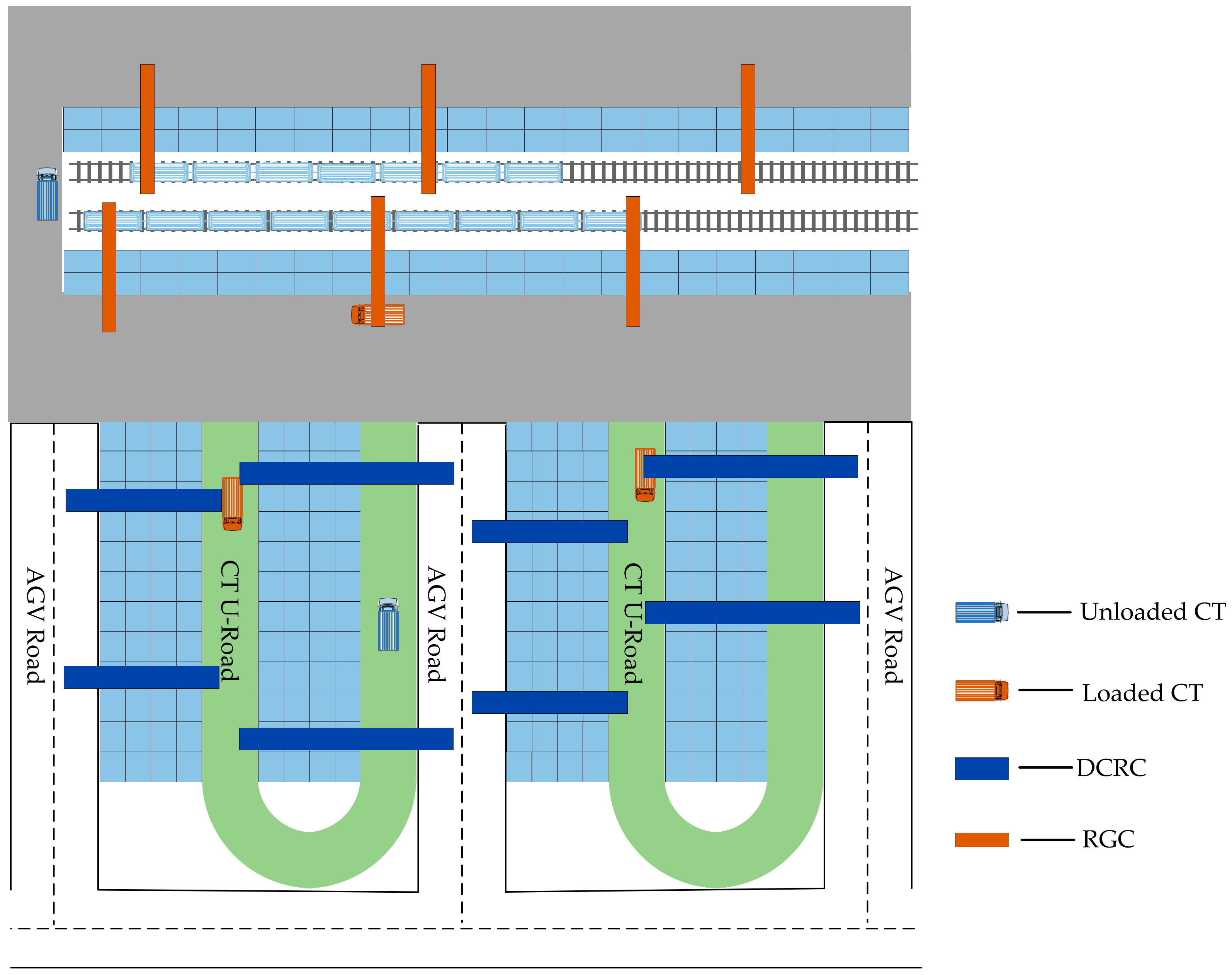
3.1. Problem Description

At U-ACT, the CTs facilitate container transfers for both the RGC in the RY and the DCRC in the UY, handling both import and export containers. Export containers arrive at the RY by train, where the RGCs load them onto CTs, which then transport them to designated storage points in the UY. Import containers, stored in the UY, are loaded onto CTs by the DCRC and transported to designated storage points in the RY. Based on the characteristics of U-ACT, the following decisions can be made:

• Scheduling of DCRC: The UY consists of multiple container blocks, each equipped with two DCRCs. Unlike traditional operations, DCRCs do not have to return to the ends of the yard after each operation. Instead, they can conduct loading and unloading operations directly inside the yard. This approach can effectively reduce the idle time of the DCRC, which effectively improves the efficiency of the operation and reduces its energy consumption.
• Scheduling of CTs: The utilization rate of CTs is related to the efficiency and energy consumption of the overall operation. Therefore, the idle distance of CTs should be minimized. CTs should be allowed to transport export containers and import containers alternately, forming a double-cycle pattern.
• Scheduling of RGC: U-ACT is equipped with yards for train operation, and each yard is equipped with three RGCs. Normally, the train transporting export containers will arrive at the terminal in advance and temporarily be stored in the RY through the RGC. The operations of the RGC are in side loading and unloading mode, which can reduce the waiting time of CT and the empty time of RGC. This mode effectively improves the operation efficiency and reduces the operation’s energy consumption.
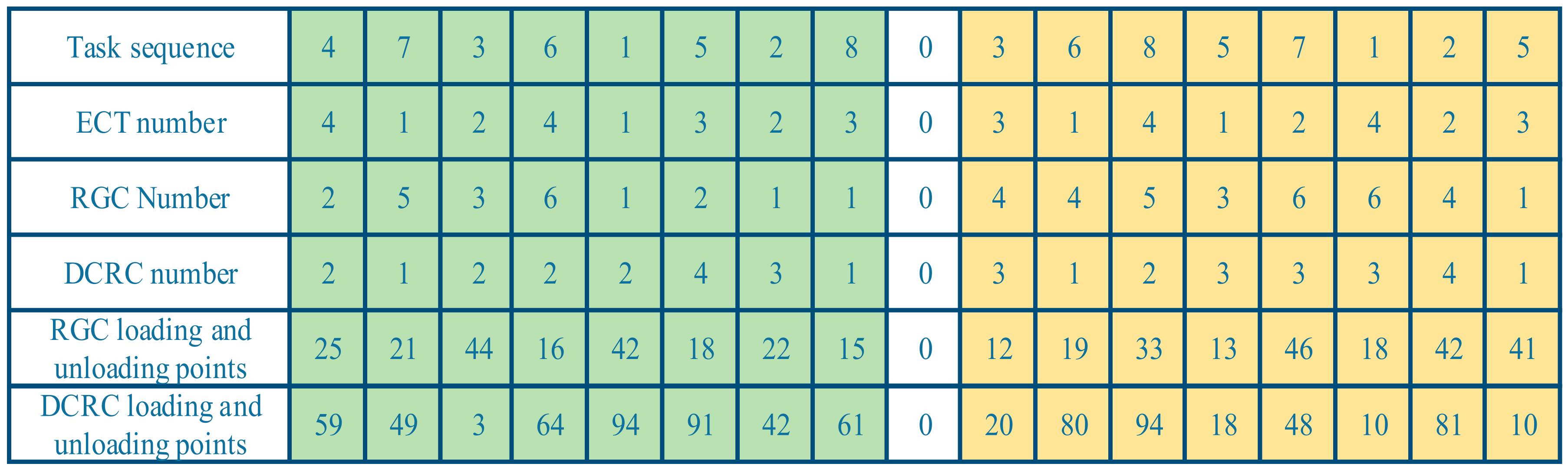
• Assignment of tasks: Task assignment in U-ACT is flexible, encompassing both the selection of CTs and the sequencing of tasks. Therefore, tasks should be distributed as evenly as possible to avoid congestion caused by centralized operations.

3.2. Assumptions

Given that the integrated scheduling problem of RGCs, CTs, and DCRCs in container transshipment at U-ACT is a complex NP-hard problem, making reasonable assumptions can facilitate its resolution:

• Each CT, RGC, and DCRC can handle only one container at a time.
• The operating speeds of CTs, RGCs, and DCRCs are known and remain constant.
• The transshipment of containers within the yard is not considered.
• All container storage points can be determined according to the distribution plan.

3.3. Notations

The notations of the model are shown in

Table 1. Sets and parameters.

Notation	Description of Notation
$I$	Set of import containers to be transferred
$O$	Set of export containers to be transferred
$C_e$	Set of containers to be transported by CT
$C$	Set of all containers, $C=I\cup O$, indexed by $i,i\prime \in C$
$E$	Set of CTs, indexed by $e,e^{\prime }\in E$
$R$	Set of RGCs, indexed by $r,r^{\prime }\in R$
$Y$	Set of DCRCs, indexed by $y,y^{\prime }\in Y$
$C_y$	Set of DCRC Tasks
$C_r$	Set of RGC Tasks
$K$	Set of paths, indexed by $k\in K$
$M$	Set of nodes, indexed by $j,j^{\prime }\in M$
$M_i^{start}$	The starting node of the container $i$
$M_i^{end}$	The destination node for the container $i$
$M_k$	Set of all nodes on the path $k$
$T_{M_k}$	Set of times for CT to reach all nodes on the path $k$
$M_{(k_1,k_2)}$	Set of conflicting nodes in space for path $k_1$ and path $k_2$
$T_{M_{(k_1,k_2)}}$	Set of times for CT to reach conflicting nodes in path $k_1$ and path $k_2$
$v_e$	Speed of CT
$v_r$	Speed of RGC
$v_y$	Speed of DCRC
$f_e$	Energy consumption per unit time for CT operation
$f_{ew}$	Energy consumption per unit time for CT waiting
$f_r$	Energy consumption per unit time for RGC operation
$f_c$	Energy consumption per unit time for DCRC operation
$m_i$	RGC processing time for container $i$
$n_i$	DCRC processing time for container $i$
$d_{j{j}^{\prime }}$	Distance from node $j$. to node $j^{\prime }$

,

Table 2. Non-decision variables.

Notation	Description of Notation
$E_1$	Total energy consumption of CT
$E_2$	Total energy consumption of DCRC
$E_3$	Total energy consumption of RGC
$a_i$	The time when CT arrives at the designated loading point for the container $i$
$p_i$	The time when CT starts processing the container $i$, which means the CT receives the container from the RGC or DCRC
$s_i$	The time when CT arrives at the designated unloading point for the container $i$
$q_i$	The time when CT completes the container task $i$
$s_i^y$	The time when DCRC $y$. moves to the designated loading and unloading point of the container $i$
$p_i^y$	The time when DCRC $y$ begins processing the container $i$
$q_i^y$	The time when DCRC $y$ completes processing the container $i$
$s_i^r$	The time when RGC $r$ moves to the designated loading and unloading point of the container $i$
$p_i^r$	The time when RGC $r$ begins processing the container $i$
$q_i^r$	The time when RGC $r$ completes processing the container $i$
$T_e$	The total time for CTs to complete container transfers
$t_{jj\prime }^k$	The time taken by CT to choose path $k$ from node $j$ to $j\prime$
$\stackrel{-}{L}$	When a path conflict occurs for the CT, the distance that needs to be passed by changing speed
$L_{safe}$	The safe distance between two CTs

and

Table 3. Decision variables.

Notation	Description of Notation
${\delta }_i^e$	When the container $i$ is to be transferred by CT $e$, ${\delta }_i^e=1$, otherwise ${\delta }_i^e=0$
$a_{j,j^{\prime }}^e$	When CT $e$. passes node $j$ and then passes through node $j^{\prime }$, $a_{j,j^{\prime }}^e=1$, otherwise $a_{j,j^{\prime }}^e=0$
$x_{i{i}^{\prime }}^e$	When the CT $e$ performs container task $i$ and then performs container task $i^{\prime }$$, x_{i{i}^{\prime }}^e=1$ otherwise, $x_{i{i}^{\prime }}^e=0$
$x_{i{i}^{\prime }}^y$	When the DCRC $y$ performs container task $i$ and then performs container task $i^{\prime }$$, x_{i{i}^{\prime }}^y=1$; otherwise, $x_{i{i}^{\prime }}^y=0$
$x_{i{i}^{\prime }}^r$	When the RGC $r$ performs container task $i$ and then performs container task $i^{\prime }$$, x_{i{i}^{\prime }}^r=1$; otherwise, $x_{i{i}^{\prime }}^r=0$

.

3.4. Integrated Scheduling Model

The integrated scheduling model aims to optimize equipment task assignment at U-ACT, primarily coordinating the operation sequence and resources of CT, RGC, and DCRC. Through the implementation of a rational scheduling scheme, the efficient coordination of multiple devices can be ensured to complete tasks while simultaneously minimizing both completion time and energy consumption. The objective function and model design are presented as follows:

$$\min F=\rho F_1+(1-\rho )F_2$$

(1)

$$F_1=\underset{i\in C}{\max }\left\{q_i^y,q_i^r\right\}$$

(2)

$$F_2=E_1+E_2+E_3$$

(3)

The objective function and model design are as follows. Equation (1) aims to minimize the objective function $F$, which consists of two components: the completion time and the total operational energy consumption. $\rho$ is a weight parameter used to adjust the preference. In Equation (2), $F_1$ represents the completion time, which is determined by the RGC or DCRC that completes the last container task. In Equation (3), $F_2$ represents the total operational energy consumption, which is composed of the energy consumption of the AGV operations, DCRC operations, and RGC operations.

$$\begin{array}{l}{E}_1={\displaystyle \sum _{e\in E}{\displaystyle \sum _{i,i^{\prime }\in C}[(s_i-p_i)+(a_i-q_{i^{\prime }})x_{i^{\prime }i}^e]\cdot {\delta }_i^e\cdot f_e}}\\ +{\displaystyle \sum _{e\in E}{\displaystyle \sum _{i,i^{\prime }\in C}[(p_i-a_i)+(q_i-s_i)]\cdot {\delta }_i^e\cdot f_{ew}}}\end{array}$$

(4)

$$E_2={\displaystyle \sum _{y\in Y}{\displaystyle \sum _{i,i^{\prime }\in C}(s_i^y-q_{i^{\prime }}^y)}}\cdot x_{i{i}^{\prime }}^y\cdot f_y$$

(5)

$$E_3={\displaystyle \sum _{r\in R}{\displaystyle \sum _{i,i^{\prime }\in C}(s_i^r-q_{i^{\prime }}^r)}}\cdot x_{i{i}^{\prime }}^r\cdot f_r$$

(6)

$${\displaystyle \sum _{e\in E}{\delta }_i^e}=1,\forall i\in C_e$$

(7)

$$x_{i{i}^{\prime }}^e+x_{i\prime i}^e\le 1,\forall e\in E,\forall i,i^{\prime }\in C_e,i\ne i^{\prime }$$

(8)

$$x_{i{i}^{\prime }}^r+x_{i^{\prime }i}^r\le 1, \forall r\in R, \forall i, i^{\prime }\in C_r, i\ne i^{\prime }$$

(9)

$$x_{i{i}^{\prime }}^y+x_{i^{\prime }i}^y\le 1, \forall y\in Y, \forall i, i^{\prime }\in C_y, i\ne i^{\prime }$$

(10)

Constraints (4)–(6) are the energy consumption calculations for CT, RGC, and DCRC, respectively. Constraint (7) ensures that each container is assigned to only one CT for transshipment. Constraints (8)–(10) ensure that CT, RGC, and DCRC operations are continuous and conflict-free.

$${\displaystyle \sum _{i\in C_e}{x}_{0i}^e}=1, \forall e\in E$$

(11)

$${\displaystyle \sum _{i\in C_e}{x}_{i0}^e}=1, \forall e\in E$$

(12)

$${\displaystyle \sum _{i\in C_r}{x}_{0i}^r}=1, \forall r\in R$$

(13)

$${\displaystyle \sum _{i\in C_r}{x}_{i0}^r}=1, \forall r\in R$$

(14)

$${\displaystyle \sum _{i\in C_y}{x}_{0i}^y}=1, \forall y\in Y$$

(15)

$${\displaystyle \sum _{i\in C_y}{x}_{i0}^y}=1, \forall y\in Y$$

(16)

$${\displaystyle \sum _{e\in E}{\displaystyle \sum _{i\in C_e\cup \left\{0\right\}}{x}_{i{i}^{\prime }}^e}=1, \forall i^{\prime }\in C_e}$$

(17)

$${\displaystyle \sum _{e\in E}{\displaystyle \sum _{i^{\prime }\in C_e\cup \left\{0\right\}}{x}_{i{i}^{\prime }}^e}=1, \forall i\in C_e}$$

(18)

$${\displaystyle \sum _{r\in R}{\displaystyle \sum _{i\in C_r\cup \left\{0\right\}}{x}_{i{i}^{\prime }}^r}=1, \forall i^{\prime }\in C_r}$$

(19)

$${\displaystyle \sum _{r\in R}{\displaystyle \sum _{i^{\prime }\in C_r\cup \left\{0\right\}}{x}_{i{i}^{\prime }}^r}=1, \forall i\in C_r}$$

(20)

$${\displaystyle \sum _{y\in Y}{\displaystyle \sum _{i\in C_y\cup \left\{0\right\}}{x}_{i{i}^{\prime }}^y}=1, \forall i^{\prime }\in C_y}$$

(21)

$${\displaystyle \sum _{y\in Y}{\displaystyle \sum _{i^{\prime }\in C_y\cup \left\{0\right\}}{x}_{i{i}^{\prime }}^y}=1, \forall i\in C_y}$$

(22)

$${\displaystyle \sum _{i\in C_e\cup \left\{0\right\}}{x}_{i{i}^{\prime }}^e}={\displaystyle \sum _{i^{″}\in C_e\cup \left\{0\right\}}{x}_{i^{\prime }{i}^{″}}^e}, \forall e\in E, \forall i^{\prime }\in C_e$$

(23)

$${\displaystyle \sum _{i\in C_r\cup \left\{0\right\}}{x}_{i{i}^{\prime }}^r}={\displaystyle \sum _{i^{″}\in C_r\cup \left\{0\right\}}{x}_{i^{\prime }{i}^{″}}^r}, \forall r\in R, \forall i^{\prime }\in C_r$$

(24)

$${\displaystyle \sum _{i\in C_y\cup \left\{0\right\}}{x}_{i{i}^{\prime }}^y}={\displaystyle \sum _{i^{″}\in C_y\cup \left\{0\right\}}{x}_{i^{\prime }{i}^{″}}^y}, \forall y\in Y, \forall i^{\prime }\in C_y$$

(25)

Constraints (11)–(16) ensure that there is one starting task and one ending task for each CT, RGC, and DCRC. Constraints (17)–(22) ensure that for each operational task of the CT, RGC, and DCRC, there is one and only one immediately preceding task and one succeeding task. Constraints (23)–(25) ensure that the container flow is balanced.

$${\displaystyle \sum _{r\in R}(q_{i^{\prime }}^r+d_{j^{\prime }j}/v_r)\cdot x_{i^{\prime }i}^r}=s_i^r, \forall i\in O, i^{\prime }\in C_r, \forall j^{\prime }\in M_{i^{\prime }}^{end}, j\in M_i^{start}$$

(26)

$$s_i^r=p_i^r, \forall i\in O, \forall r\in R$$

(27)

$$p_i^r+m_i\le q_i^r, \forall i\in O, \forall r\in R$$

(28)

$${\displaystyle \sum _{e\in E}(q_{i^{\prime }}+t_{j{j}^{\prime }}^k)\cdot x_{i^{\prime }i}^e}=a_i, \forall i\in O, i^{\prime }\in I, \forall k\in K, \forall j^{\prime }\in M_{i^{\prime }}^{end}, j\in M_i^{start}$$

(29)

$$a_i\le q_i^r, \forall i\in O, \forall r\in R$$

(30)

$$p_i=q_i^r, \forall i\in O, \forall r\in R$$

(31)

Constraints (26)–(31) are constraints on the time before the CT $e$ starts transferring the export container $i$. Constraint (26) defines the time when the RGC $r$ moves to the loading point of the container $i$ after completing the previous task. Constraint (27) is the time when the RGC $r$ starts moving the export container $i$. Constraint (28) ensures that the time when RGC $r$ completes the export container task $i$ is not earlier than the time required for handling. Constraint (29) defines the time for the CT $e$ to move to the loading point of the export container $i$ after completing the previous task. Constraint (30) ensures that the time when the RGC $r$ completes the export container task $i$ is not earlier than the arrival time of the CT $e$. Constraint (31) implies that the time when the RGC $r$ completes the export container task $i$ is equal to the time when the CT starts transferring the export container $i$.

$$p_i+{\displaystyle \sum _{e\in E}{t}_{j{j}^{\prime }}^k\cdot {\delta }_i^e}=s_i, \forall i\in O\cap C_e, \forall k\in K, \forall j\in M_i^{start}, j^{\prime }\in M_i^{end}$$

(32)

$${\displaystyle \sum _{y\in Y}(q_{i^{\prime }}^y+d_{j^{\prime }j}/v_y)\cdot x_{i^{\prime }i}^y}=s_i^y, \forall i\in O, i^{\prime }\in C_y, \forall j\in M_i^{end}, j^{\prime }\in M_{i^{\prime }}^{end}$$

(33)

$$p_i^y=\max \left\{s_i^y,s_i\right\}, \forall i\in O, \forall y\in Y$$

(34)

$$q_i=p_i^y, \forall i\in O, \forall y\in Y$$

(35)

$$p_i^y+n_i=q_i^y, \forall i\in O, \forall y\in Y$$

(36)

Constraints (32)–(36) are constraints on the temporal relationship of the export container tasks between CT and DCRC. Constraint (32) constrains the time when the CT $e$ moves the export container $i$ to the designated unloading point. Constraint (33) defines the time when the DCRC $y$ moves to the unloading point of the export container $i$ after completing the previous task. Constraint (34) ensures that the DCRC $y$ starts moving the export container $i$ no earlier than the arrival time of the CT $e$ and the arrival time of the DCRC $y$. Constraint (35) implies that the CT $e$ completes its current task when the DCRC $y$ starts moving the export container $i$. Constraint (36) defines the time when the DCRC $y$ finishes moving the export container $i$.

$${\displaystyle \sum _{y\in Y}(q_{i^{\prime }}^y+d_{j^{\prime }j}/v_y)\cdot x_{i^{\prime }i}^y}=s_i^y, \forall i\in I, i^{\prime }\in C_y, \forall j^{\prime }\in M_{i^{\prime }}^{end}, j\in M_i^{start}$$

(37)

$$s_i^y=p_i^y, \forall i\in I, \forall y\in Y$$

(38)

$$p_i^y+n_i\le q_i^y, \forall i\in I, \forall y\in Y$$

(39)

$${\displaystyle \sum _{e\in E}(q_{i^{\prime }}+t_{j{j}^{\prime }}^k)\cdot x_{i^{\prime }i}^e}=a_i, \forall i\in I, i^{\prime }\in O, \forall k\in K, \forall j^{\prime }\in M_{i^{\prime }}^{end}, j\in M_i^{start}$$

(40)

$$a_i\le q_i^y, \forall i\in I, \forall y\in Y$$

(41)

$$p_i=q_i^y, \forall i\in I, \forall y\in Y$$

(42)

Constraints (37)–(42) are constraints on the time before the CT $e$ starts transferring the import container $i$. Constraint (37) defines the time when the DCRC $y$ moves to the loading point of the import container $i$ after completing the previous task. Constraint (38) is the time when the DCRC $y$ starts moving the import container $i$. Constraint (39) ensures that the DCRC $y$ completes the import container task $i$ not earlier than the time required for handling. Constraint (40) defines the time for the CT $e$ to move to the loading point of the import container task $i$ after completing the previous task. Constraint (41) ensures that the time when the DCRC $y$ completes the import container task $i$ is not earlier than the arrival time of the CT $e$. Constraint (42) implies that the time when the DCRC $y$ completes the import container task $i$ is equal to the time when the CT $e$ starts transferring the import container $i$.

$$p_i+{\displaystyle \sum _{e\in E}{t}_{j{j}^{\prime }}^k\cdot {\delta }_i^e}=s_i, \forall i\in I\cap C_e, \forall k\in K, \forall j\in M_i^{start}, j^{\prime }\in M_i^{end}$$

(43)

$${\displaystyle \sum _{r\in R}(q_{i\prime }^r+d_{j^{\prime }j}/v_r)\cdot x_{i^{\prime }i}^r}=s_i^r, \forall i\in I, i^{\prime }\in C_r, \forall j\in M_i^{end}, j^{\prime }\in M_{i^{\prime }}^{end}$$

(44)

$$p_i^r=\max \left\{s_i^r,s_i\right\}, \forall i\in I, \forall r\in R$$

(45)

$$q_i=p_i^r, \forall i\in I, \forall r\in R$$

(46)

$$p_i^r+n_i=q_i^r, \forall i\in I, \forall r\in R$$

(47)

Constraints (43) and (44) are constraints on the temporal relationship of the import container tasks between CT and RGC. Constraint (43) constrains the time when the CT $e$ moves the import container $i$ to the designated unloading point. Constraint (44) defines the time when the RGC $r$ moves to the unloading point of the import container task $i$ after completing the previous task. Constraint (45) ensures that the time when the RGC $r$ starts moving the import container $i$ is not earlier than the arrival time of the CT $e$ and the arrival time of the RGC $r$. Constraint (46) implies that the CT $e$ completes its current task when the RGC $r$ starts moving the import container $i$. Constraint (47) defines the time when the RGC $r$ finishes moving the import container $i$.

$$a_i, p_i, s_i, q_i, p_i^y, q_i^y, s_i^r, p_i^r, q_i^r, t_{j{j}^{\prime }}^k\ge 0$$

(48)

$$a_{j,j^{\prime }}^e, {\delta }_i^e, x_{i{i}^{\prime }}^e, x_{i{i}^{\prime }}^y, x_{i{i}^{\prime }}^r\in \left\{0,1\right\}$$

(49)

Constraints (48) and (49) ensure the scope of individual variables.

3.5. Path Planning Model

The path planning model is responsible for optimizing the travel path of a CT in a U-ACT. As a key horizontal transportation equipment in the transshipment process, the travel path of the CT has a great impact on the operation. Selecting the right route can greatly reduce the travel time of the CT. Under the U-shaped layout, the use of unidirectional pathways can decrease the occurrence of conflicts. The traffic area can be divided into a topological network consisting of 238 nodes. Connections between nodes represent passable paths as shown in Figure 2.

CT conflicts may occur during transportation. Conflicts can be divided into node conflicts during transportation and occupancy conflicts at loading and unloading points. When a conflict occurs, the CT is controlled to accelerate, decelerate, or stop and wait to avoid collisions. Therefore, the model is established with the objective of minimizing travel time and considering vehicle conflicts.

$$\min T_e={\displaystyle \sum _{e\in E}{\displaystyle \sum _{k\in K}{\displaystyle \sum _{i\in I}{t}_{j{j}^{\prime }}^k\cdot }}}{\delta }_i^e$$

(50)

Subject to

$${\displaystyle \sum _{j,j^{\prime }\in M}{\displaystyle \sum _{i\in C}{a}_{j,j^{\prime }}^e\cdot {\delta }_i^e=1}, \forall e\in E}$$

(51)

$${\displaystyle \sum _{j,j^{\prime }\in M}{\displaystyle \sum _{i\in C}{a}_{j,j^{\prime }}^e\cdot {\delta }_i^e}}-{\displaystyle \sum _{j,j^{\prime }\in M}{\displaystyle \sum _{i\in C}{a}_{j^{\prime },j}^e\cdot {\delta }_i^e}=\{\begin{array}{l}1,j\in O_i\\ 0,other\\ -1,j\in {O_i}^{\prime }\end{array}, \forall e\in E}$$

(52)

Since the paths are unidirectional at the U-ACT, constraint (51) means that the CT does not pass through a node repeatedly during a transshipment. Constraint (52) ensures that the node flow is balanced.

$$M_{(k_1,k_2)}=M_{k_1}\cap M_{k_2}$$

(53)

$$T_{M_{(k_1,k_2)}}=T_{M_{k_1}}\cap T_{M_{k_2}}$$

(54)

$$\stackrel{-}{L}=(L_{safe}+{\displaystyle \frac{v_0^2-v_e^2}{2a}})$$

(55)

$$t_{com}=(v_0-v_e)/a-\stackrel{-}{L}/v_0$$

(56)

$$t_{j{j}^{\prime }}^k={\displaystyle \sum _{\begin{array}{l}j\in M_i^{start},\\ j^{\prime }\in M_i^{end}\end{array}}{\displaystyle \sum _{i\in I}(d_{j{j}^{\prime }}\cdot {\delta }_i^e)/v_e}}+t_{com}$$

(57)

The constraint (53) means detecting whether there is a conflicting section between two paths. Constraint (54) means detecting whether there is a temporal conflict between two conflicting paths. Constraint (55) means that when two CTs are in spatial-temporal conflict, the path conflict is resolved by accelerating and decelerating under a guaranteed safe distance. Vehicles with high priority speed up to pass, and vehicles with low priority slow down to pass. $v_0$ represents the changed velocity. Constraint (56) indicates the time compensation. Constraint (57) defines the time taken by the CT $e$ to select the path $k$ to complete the transshipment of the container $i$.

$${(t_{In,ki})}_{je}<{(t_{In,k^{\prime }{i}^{\prime }})}_{j(e+1)}, \forall i, i^{\prime }\in I, \forall k, k^{\prime }\in K, \forall e\in E, \forall j\in M_i^{start}\cup M_i^{end}$$

(58)

$${(t_{Out,ki})}_{je}<{(t_{Out,k^{\prime }{i}^{\prime }})}_{j(e+1)}, \forall i, i^{\prime }\in I, \forall k, k^{\prime }\in K, \forall e\in E, \forall j\in M_i^{start}\cup M_i^{end}$$

(59)

Constraints (58) and (59) represent the temporal relationship between two consecutive CTs leaving or arriving at the same loading and unloading point.

4. Solution Approach

Numerous heuristic algorithms have been developed for the integrated scheduling problem of ACT. For example, Song et al. [36] addressed flexible AGV scheduling under a charging strategy using an Adaptive Large Neighborhood Search algorithm (ALNS), while Yang et al. [37] proposed an Adaptive Co-evolutionary Genetic Algorithm (ACGA) to optimize DCRC operations at U-ACT. However, selecting the most suitable algorithm for a specific scheduling problem remains challenging.

This paper proposes a hyper-heuristic algorithm, reinforcement learning-driven hyper-heuristic algorithm (RLHA), which incorporates the idea of reinforcement learning to dynamically adapt to complex scheduling problems. The incorporation of reinforcement learning endows RLHA with enhanced adaptability, demonstrating superior performance in handling multifaceted scheduling challenges compared to traditional algorithms.

RLHA is designed with a three-layer structure: a selection layer, a scheduling layer, and a path planning layer. The selection layer applies reinforcement learning to choose the appropriate heuristic algorithm based on problem characteristics; the scheduling layer performs computations using the selected heuristic; and the path planning layer determines the transportation path for CTs. Leveraging the idea of reinforcement learning, RLHA efficiently searches for scheduling schemes within a complex solution space. The process is illustrated in Figure 3.

4.1. Selection Layer Algorithm Design

4.1.1. Hyper-Heuristic Algorithm

The core principle of the hyper-heuristic algorithm (HHA) lies in dynamically selecting low-level heuristic algorithms to address complex optimization problems through adaptive strategy mechanisms. Unlike traditional heuristic algorithms that operate within specific problem solution spaces, HHA orchestrates the selection, combination, and adaptation of low-level heuristics [38]. In this paper, the heuristic algorithms are selected based on weights:

$$P_i=w_i/{\displaystyle \sum _{j=1}^n{w}_j}$$

(60)

$P_i$ is the probability of selecting the $i$ heuristic algorithm, and $w_i$ is the weight of that heuristic algorithm. The weights are dynamically adjusted to control the probability that a heuristic algorithm is selected.

The weight parameters can be updated. In this paper, we combine the Q-value in reinforcement learning as an update strategy, and the equation is:

$${w_i}^{\prime }=w_i+R(s,a,s^{\prime })$$

(61)

$w_i$ is the current weights, ${w_i}^{\prime }$ is the updated weights, and $R(s,a,s^{\prime })$ is the reward value obtained from the algorithm performance. Reward value is higher, and algorithm performance is better.

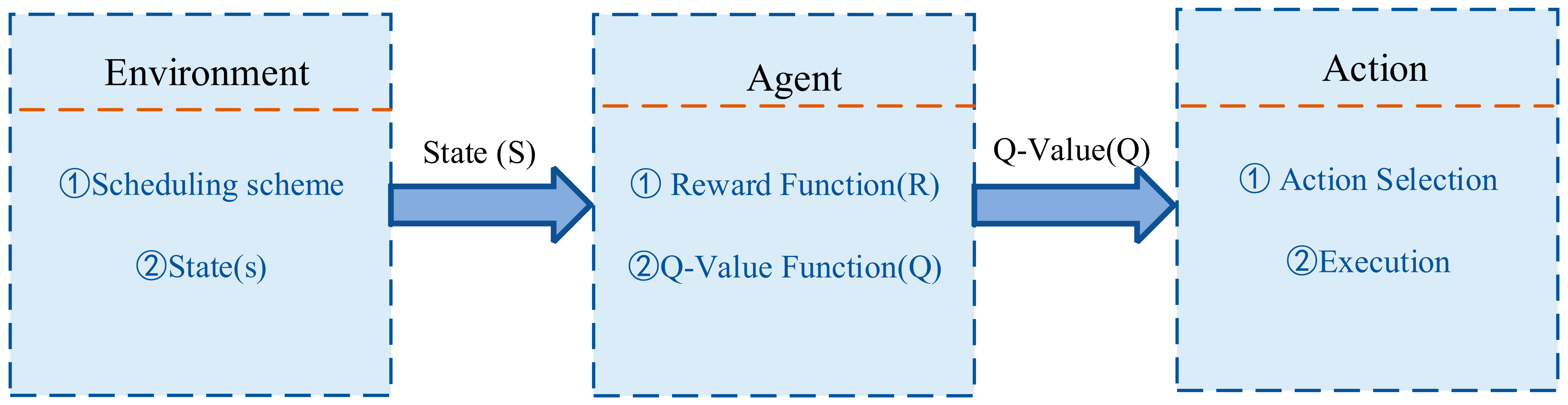
4.1.2. Q-Learning Algorithm

Q-learning is a classical reinforcement learning algorithm. The key components of Q-learning include state, action, reward function, and Q-value update mechanism, as shown in Figure 4 [39].

In this study, the Q-learning principle is only utilized as the selection mechanism of the hyper-heuristic algorithm, without involving Q-learning training. During each iteration of the hyper-heuristic algorithm, the solution generated is compared with the solution from the previous iteration. The weight of the selected heuristic algorithm is then updated based on the reward function. As the problem pertains to scheduling, the reward evaluates the quality of the scheduling result obtained by applying the current heuristic algorithm.

In reinforcement learning, state and action are two core concepts. The state is a variable that describes the current situation of a system. In this paper, state is reflected as the completion time and energy consumption. The state space can be defined as $S=\left\{\mathrm{Completion} \mathrm{Time},\mathrm{Energy} \mathrm{Consumption}\right\}$. Action is how an agent interacts with the environment. In this paper, action is reflected as the selection of heuristic algorithms for computation. The action space can be defined as $A=\{\mathrm{GA},\mathrm{AGA},\mathrm{ALNS},\dots \}$:

Each time a heuristic algorithm is selected and executed, a reward value is assigned based on the scheduling results. Accordingly, the reward function can be defined as:

$$R(s,a,s^{\prime })=-\alpha \cdot F(s^{\prime })+\beta \cdot \Delta F$$

(62)

$\alpha$ and $\beta$ are weight parameters, and $F(s^{\prime })$ is the objective value in state $s^{\prime }$. The objective value is obtained from the completion time and energy consumption in the state space. $\Delta F$ is the amount of change in the objective value.

The formula for updating the Q value is as follows:

$$Q(s,a)\leftarrow (1-\theta )\cdot Q(s,a)+\theta \cdot [R(s,a,s^{\prime })+\gamma \cdot {\max }_{a^{\prime }}Q(s^{\prime },a^{\prime })]$$

(63)

$Q(s,a)$ is the Q-value of performing action $a$ in state $s$. $s^{\prime }$ represents the next state of the agent after performing action $a$. $a^{\prime }$ represents the next action selected by the agent in the new state $s^{\prime }$. ${\max }_{a^{\prime }}Q(s^{\prime },a^{\prime })$ represents the selection of an action $a^{\prime }$ that maximizes the Q-value in the new state $s^{\prime }$. $R(s,a,s^{\prime })$ is the reward value after performing action $a$. $\gamma$ is the discount factor, and $\theta$ is the learning rate.

The $\epsilon$-greedy policy is used to select the next action:

$$\mathrm{Select} \mathrm{Action}\{\begin{array}{l}\mathrm{Randomly} \mathrm{Select} \mathrm{Action} a if \mathrm{rand}\le \epsilon \\ \arg {\max }_{a}Q(s,a) \mathrm{otherwise}\end{array}$$

(64)

The learning rate can be set to:

$${\theta }_t={\theta }_0(1-t/T)$$

(65)

${\theta }_t$ is the learning rate at $t$ iterations, ${\theta }_0$ is the initial learning rate, $T$ is the total number of iterations.

The HHA based on Q-learning can achieve significant performance improvement in solving complex optimization problems by combining the learning ability of reinforcement learning and the property of heuristic algorithms to search for global solutions. The steps are as follows:

I.

The Q-value is initialized and all state-actions are set to zero.

II.

The heuristic algorithm is selected based on the selection layer. Then, solve and compute the model described in Chapter 3 to generate the current solution.

III.

Based on the results of the scheduling program, the reward value is calculated and the Q-value is updated.

IV.

Iterate and optimize the scheduling scheme until the termination criteria are reached.

4.2. Scheduling Layer Algorithm Design

In this paper, seven distinct heuristic algorithms were developed: Single-Point Crossover Genetic Algorithm (SPCGA), Multi-Point Crossover Genetic Algorithm (MPCGA), Greedy Strategy Genetic Algorithm (GSGA), Adaptive Genetic Algorithm (AGA), Co-evolutionary Genetic Algorithm (CGA), Simulated Annealing Algorithm (SA), and Adaptive Large Neighborhood Search Algorithm (ALNS).

The scheduling layer algorithm is determined by the action values generated from the selection layer, while the scheduling layer’s output solution, in turn, updates the Q-values in the selection layer, forming an interdependent relationship between the two layers. The primary objective is to minimize job completion time and energy consumption, ultimately achieving the optimal scheduling solution.

As GA, SAA, and ALNS typically use integer and sequential coding for scheduling problems, the solution employs a unified chromosome coding scheme, as illustrated in Figure 5. This multilayer chromosome structure can also be represented as a matrix, where the green section denotes export container tasks and the yellow section indicates import container tasks, separated by ‘0’.

4.3. Path Planning Layer Algorithm Design

CTs require path planning. Based on the topology diagram in Figure 2, this paper applied the Dijkstra algorithm to find the shortest path for CTs in transshipment tasks. Conflicts between CTs are then detected both spatially and temporally. Conflict types are divided into two categories: node conflicts and occupancy conflicts. A node conflict, a spatiotemporal conflict, occurs when CTs arrive at the same node simultaneously. In such cases, vehicles closer to the endpoint are given higher priority, accelerating to pass, while those further from the endpoint decelerate. An occupancy conflict arises when a CT arrives at a loading/unloading point already occupied by another vehicle; in this case, the CT must wait for the preceding vehicle to complete its operation.

The path planning layer is related to the task sequence output from the scheduling layer. In turn, the CT paths obtained by the path planning layer affect the scheduling plan of the scheduling layer. Therefore, the two layers are interdependent.

5. Simulation Experiments and Analysis

This section verifies the validity of the model and algorithm through computational experiments. RLHA is implemented through MATLAB 2020b running on the WINDOW11 operating system, Intel (R) Core (TM) i7-10875H CPU @ 2.30 GHz, 16 GB RAM. A small-scale experiment and a large-scale experiment were set up; the results of the small-scale experiment were used to verify the validity of RLHA, while the results of the large-scale experiment were used for the operational analysis of the terminal.

5.1. Parameter Design

The data design in this paper is based on an actual survey conducted at the Qinzhou Automated Container Terminal in Beibu Gulf. This terminal is the first in the world to apply a U-shaped layout. The U-ACT investigated in this study is set up with two stacking areas at the RY, and each area is equipped with three RGCs. Four container blocks are considered at the UY yard, each with 100 available bays and equipped with two DCRCs. The number of available CTs is 10~20. The speed of CT is 5 m/s and the energy consumption is 0.05 kWh/s. The speed of RGC is 1 m/s and the energy consumption is 0.025 kWh/s. The speed of DCRC is 1 m/s and the energy consumption is 0.03 kWh/s. The tasks to be processed are 20~2000. The time for RGC to process a container obeys the uniform distribution of (20 s, 30 s) and the time for DCRC to process a container obeys the uniform distribution of (30 s, 40 s).

The mixed integer model established in this paper includes minimizing the completion time of container transshipment and the total energy consumption of multiple automated devices. The objective function can be processed as shown in Equation (1).

5.2. Algorithm Comparison

This section verifies the feasibility of the proposed model and algorithm through small-scale experiments. We compare the RLHA algorithm with GA, CGA, ALNS, and BCOHH. These algorithms represent well-established benchmarks in optimization research. The performance of the five algorithms is analyzed based on objective value (OBJ) and required computation time (CPT). The value of $\rho$ in the small-scale experiment is 0.3. The number of CTs enabled is 10 and 20, the number of RGCs enabled is 3, and the number of DCRCs enabled is 4. The number of tasks varies from 20 to 200, including import and export containers. The task interval for each set of experiments is 20, for a total of 10 sets of experiments.

The OBJ and CPT under the five algorithms are compared. Each group of experiments is conducted ten times, and the average value is taken as the result. The experimental results of 10 CTs are shown in

Table A1. Comparison of algorithms.

TASKS	CT	RGC/DCRC	Method	OBJ	CPT (s)
20	10	3/4	RLHA	927.34	46.74
			BCOHH	965.81	55.25
			ACGA	950.09	8.58
			ALNS	998.71	18.58
			GA	1057.89	12.32
40	10	3/4	RLHA	1878.76	60.03
			BCOHH	1943.36	93.26
			ACGA	1977.97	13.67
			ALNS	1779.87	26.25
			GA	2156.75	17.64
60	10	3/4	RLHA	2829.72	80.88
			BCOHH	2937.89	108.23
			ACGA	3039.62	17.51
			ALNS	2915.49	33.80
			GA	3373.20	22.41
80	10	3/4	RLHA	3791.01	108.52
			BCOHH	3957.93	140.61
			ACGA	4236.74	22.00
			ALNS	3822.37	40.80
			GA	4626.90	27.00
100	10	3/4	RLHA	4772.53	103.46
			BCOHH	5017.74	160.65
			ACGA	5531.28	25.37
			ALNS	5258.06	46.37
			GA	6150.21	32.03
120	10	3/4	RLHA	5823.69	111.12
			BCOHH	6059.06	171.26
			ACGA	6950.86	28.72
			ALNS	6442.65	52.36
			GA	7527.36	40.09
140	10	3/4	RLHA	6829.73	141.07
			BCOHH	7026.40	170.62
			ACGA	8434.83	35.04
			ALNS	7628.35	58.11
			GA	9061.73	39.10
160	10	3/4	RLHA	7979.53	125.13
			BCOHH	8220.62	235.41
			ACGA	9789.28	36.90
			ALNS	9296.57	61.79
			GA	10,640.52	44.30
180	10	3/4	RLHA	9003.86	162.26
			BCOHH	9180.67	209.34
			ACGA	11,582.00	40.42
			ALNS	10,713.51	66.14
			GA	12,315.47	64.94
200	10	3/4	RLHA	10,071.85	133.37
			BCOHH	10,516.29	273.19
			ACGA	13,258.22	45.49
			ALNS	12,488.00	70.21
			GA	14,178.40	49.78

. To explore the effectiveness of the algorithm, the scheduling results are quantitatively analyzed. The results for an average of 100 container tasks are shown in

Table 4. One-hundred evaluation indicators for container tasks scheduling.

Index	RLHA	BCOHH	ACGA	ALNS	GA
GAP	—	5.14%	15.90%	10.17%	28.87%
Completion time	3467.00	3826.00	3640.00	3761.00	3874.00
Total energy consumption	5269.66	6409.27	6341.83	6437.71	6570.58
CPT	103.46	160.65	25.37	46.37	32.03

. The table includes four key factors: GAP, completion time, total energy consumption, and CPT. The calculation method for the GAP is as follows:

$$\mathrm{GAP}={\displaystyle \frac{F_{Current}-F_{best}}{F_{best}}}\cdot 100\%$$

(66)

In Equation (66), $F_{best}$ represents the optimal objective value obtained by the five algorithms, and $F_{Current}$ represents the objective value obtained by the current algorithm.

According to the experimental results, Figure 6 can be obtained. The differences between the five algorithms can be seen in the two figures. When the number of experimental tasks is small, the difference between the OBJs obtained by the five algorithms is small. However, as the number of experimental tasks increases and the scheduling problem becomes more complex, the optimization results of RLHA and BCOHH are significantly better than the other three heuristic algorithms. The heuristic algorithm ALNS is the most effective and GA is the least effective. This is due to the fact that the heuristic algorithms fall into local optimums too early in complex situations, which leads to less effective algorithms. In contrast, HHA can escape from of the local optimum more easily while learning to find the optimum.

From the analysis of the scheduling results in Table 4, the total completion time and energy consumption of the scheduling scheme obtained by RLHA are significantly lower than those obtained by the three heuristics. Although the GAP of the results obtained by RLHA and BCOHH is small, the CPT required by RLHA is smaller. This proves the feasibility and effectiveness of RLHA in practical situations. It also proves that RLHA is a competitive algorithm.

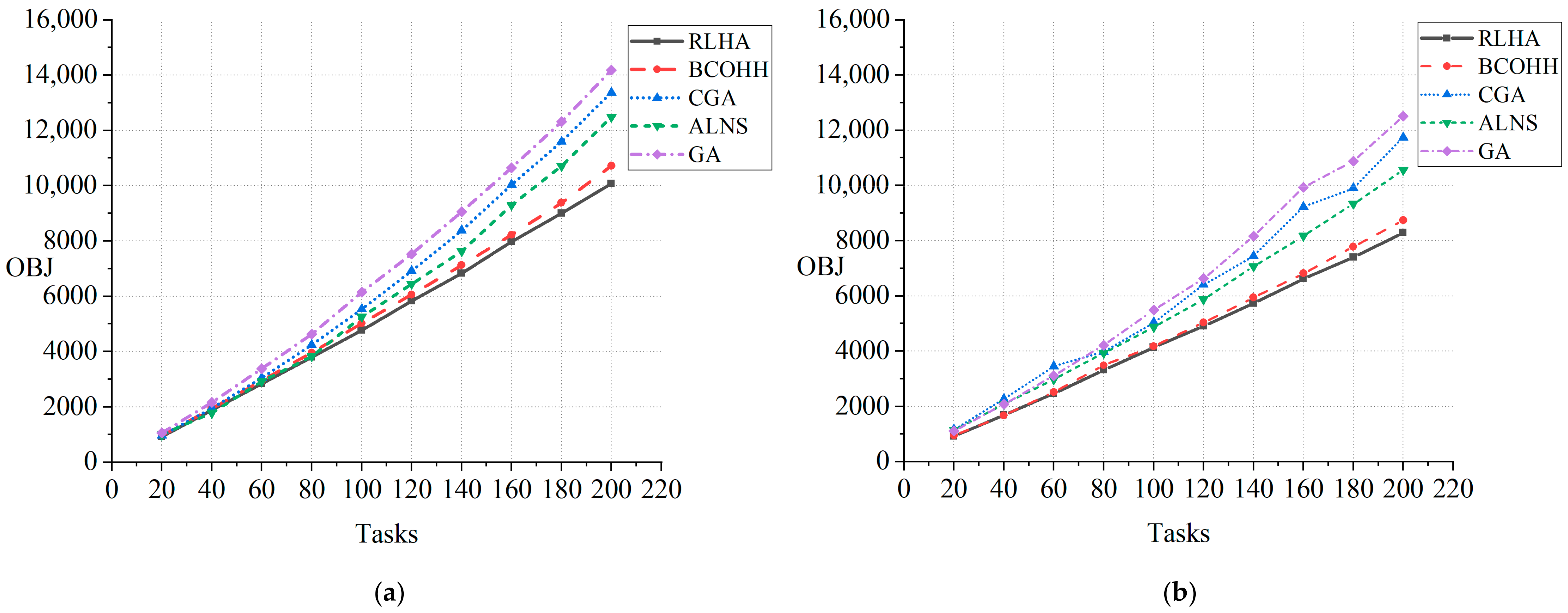
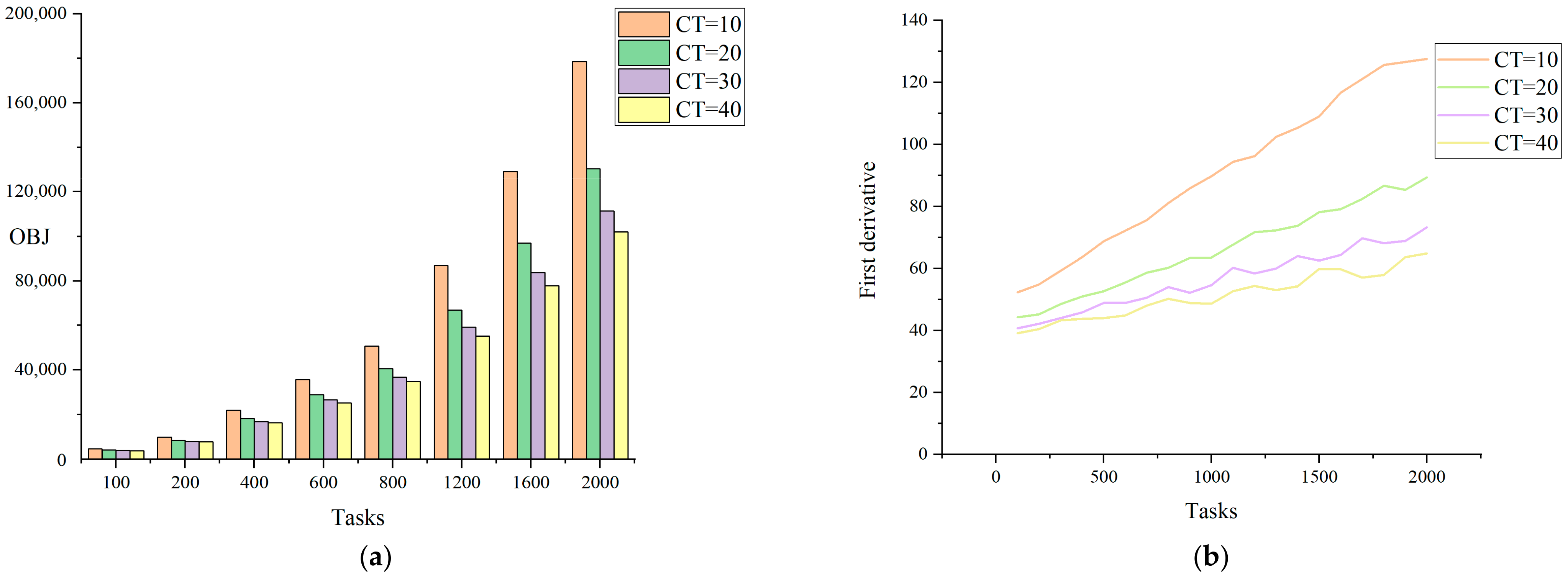
5.3. Large-Scale Experiment

Large-scale operations are common in terminal settings; therefore, the next step involves conducting a large-scale experiment with the number of container tasks ranging from 100 to 2000. In the large-scale experiment, the value of $\rho$ was set to 0.3, with six RGCs and eight DCRCs enabled. The experimental data are recorded in

Table A2. Results of large-scale experiment.

Tasks	CTs	Method	OBJ
100	10	RLHA	4763.78
200	10	RLHA	10,024.05
400	10	RLHA	21,883.57
600	10	RLHA	35,640.61
800	10	RLHA	50,747.29
1200	10	RLHA	86,803.77
1600	10	RLHA	129,084.80
2000	10	RLHA	178,611.60
100	20	RLHA	4157.00
200	20	RLHA	8583.77
400	20	RLHA	18,291.08
600	20	RLHA	28,838.55
800	20	RLHA	40,567.03
1200	20	RLHA	66,789.70
1600	20	RLHA	96,879.10
2000	20	RLHA	130,427.93
100	30	RLHA	3970.01
200	30	RLHA	8042.12
400	30	RLHA	16,841.44
600	30	RLHA	26,616.61
800	30	RLHA	36,724.70
1200	30	RLHA	59,193.52
1600	30	RLHA	83,681.12
2000	30	RLHA	111,404.48

.

The large-scale experimental results shown in Figure 7. illustrate the relationship between the OBJ, the number of tasks, and the number of CTs. Additionally, the first-order derivative of the OBJ with respect to the number of tasks is plotted. Although the function is not continuous, derivatives can be estimated using numerical difference method. The figure indicates that the OBJ is influenced by both the number of CTs and tasks. Specifically, as the number of tasks increases, the OBJ also increases. When the number of tasks is substantial, the impact of the number of CTs on the OBJ becomes particularly pronounced; a higher number of CTs corresponds to a lower OBJ. This is evident from the increasing first-order derivatives. Consequently, the subsequent analysis focuses on the relationship between the number of CTs and the OBJ.

Figure 8 illustrates the operations for varying numbers of CTs at 200, 300, and 400 container tasks. As the number of container tasks increases, the OBJ also increases. For a fixed number of container tasks, the OBJ initially decreases and then rises as the number of CTs increases. From the lowest point in the figure, it can be concluded that the OBJ reaches its minimum when the ratio of container tasks to CTs is approximately 8:1. This is due to congestion caused by an excessive number of CTs relative to the given number of RGCs and DCRCs. Therefore, deploying an optimal number of CTs significantly impacts terminal operational efficiency.

Figure 9 presents a Gantt chart illustrating the actual operation of 20 CTs. Given the large volume of 2000 container tasks, analyzing the complete Gantt chart is impractical; therefore, only a portion is shown. This excerpt allows for a focused analysis of CTs during container transshipment operations. In the figure, the array indicates that the ith vehicle is handling its jth task. The chart reveals varying time intervals: long intervals occur when a CT is transferring containers between the RY and UY, moderate intervals are observed when CTs operate between different container blocks within the same yard, and very short intervals appear when a CT operates within different bays of the same container block.

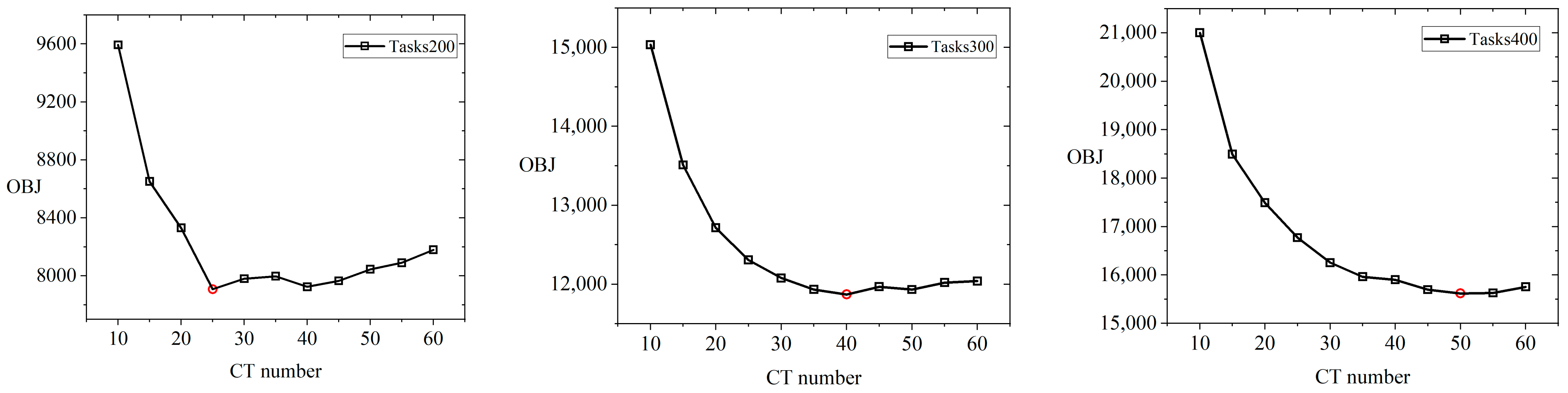
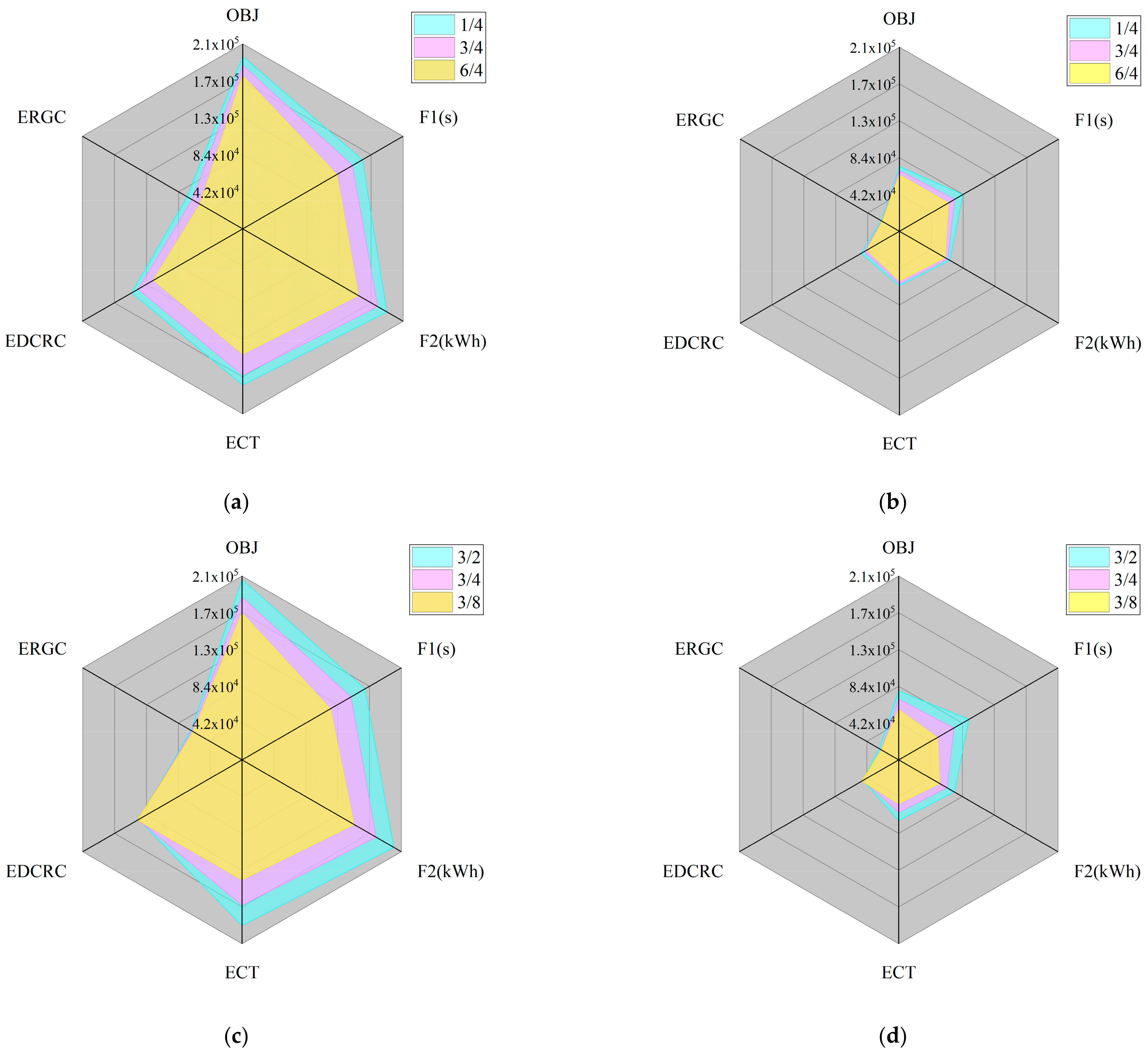
5.4. Sensitivity Analysis

The number of DCRCs and RGCs represents the capacity of the terminal to handle containers. Therefore, it is important to analyze the sensitivity of the operation to both. The large-scale experiments are conducted by adjusting the number of RGCs (1/3/6) enabled and the number of DCRCs (2/4/8) enabled, and the data are shown in

Table A3. Results of sensitivity analysis experiment.

TASKS	CT	RGC/DCRC	OBJ	F1 (s)	F2 (kWh)	ECT	EDCRC	ERGC
2000	10	1/4	195,903	74,622	251,816	236,259	10,371	5185
2000	10	3/4	185,854	68,455	235,780	221,295	9776	4709
2000	10	6/4	173,503	58,649	201,815	189,516	8334	3965
1000	10	1/4	73,814	39,876	88,511	83,197	3613	1700
1000	10	3/4	69,276	34,600	85,044	80,079	3323	1641
1000	10	6/4	64,114	30,609	80,045	75,392	3037	1615
2000	10	3/2	206,048	77,337	266,960	252,434	9736	4790
2000	10	3/4	185,854	68,455	235,780	221,295	9776	4709
2000	10	3/8	167,556	55,436	196,704	182,334	9806	4564
1000	10	3/2	78,767	44,093	97,883	92,728	3331	1824
1000	10	3/4	69,276	34,600	85,044	80,079	3323	1641
1000	10	3/8	57,073	24,322	71,693	66,650	3441	1602

. In Table A3, ECT, ERGC, and EDCRC represent the energy consumption of CT, RGC, and DCRC, respectively.

According to Table A3, a radar chart analyzing the sensitivity of RGC and DCRC quantities can be drawn, as shown in Figure 10. From the figure, it can be seen that in the case of large-scale operations, the more container loading and unloading equipment is invested, the lower the OBJ is, the shorter the overall operation time of the terminal is, and the lower the total energy consumption is. This is mainly because the more loading and unloading equipment there is, the shorter the CT waiting time is. In addition, compared to ERGC and EDCRC, ECT is more significantly influenced by the number of container handling equipment.

Based on the comparison of Figure 10a,b as well as Figure 10c,d, the same conclusion can be drawn. For the same automation equipment configuration, a larger number of tasks leads to a larger OBJ, a longer operation time, and a higher energy consumption. From the comparison of Figure 10a,c, as well as Figure 10b,d, the sensitivity of the overall operation is more sensitive to the number of DCRCs than to the number of RGCs. DCRC quantity has a greater impact on completion time and energy consumption, i.e., it has a greater impact on OBJ. This is mainly because the number of DCRCs has a greater impact on the energy consumption of the CTs during the operation, and also indicates that the CTs have more waiting situations at the DCRCs.

The overall operating time and energy consumption of the terminal are considered, where the computational preference for both is varied by changing the value of $\rho$ in Equation (2). Choose $\rho$ = 0.5 and $\rho$ = 0.7 for comparison. Figure 11 shows the results of large-scale experiments obtained by changing the value of $\rho$.

Figure 11 and Figure 7 show that the OBJ increases as the number of tasks rises. Furthermore, at a large operational scale, a reasonable allocation of CTs can significantly enhance the overall efficiency of sea-rail transportation at the terminal. However, when $\rho$ takes different values, the impact of the number of CTs and tasks on the OBJ varies. Specifically, the OBJ is less sensitive to the number of CTs when operational time is prioritized, but it is more significantly affected when energy consumption is prioritized, indicating greater sensitivity for smaller $\rho$ values. This is demonstrated by the fact that the first-order derivatives are larger when $\rho$ takes smaller values. Consequently, optimizing the U-shaped sea-rail intermodal terminal’s performance is particularly effective when energy consumption is given greater preference.

6. Conclusions

The construction of sea-rail intermodal transportation operations at U-ACT presents a new challenge amid the rapid development of intermodal transportation. This paper proposes a two-layer scheduling model. The upper layer is an integrated scheduling model for multiple equipment, and the lower layer is a CT path planning model. Considering the complexity of the model, we propose a reinforcement learning-driven hyper-heuristic algorithm. The scheduling layer efficiently calculates scheduling scenarios, including task sequences for UY and RY operations as well as coordination among the three automated devices. The selection layer evaluates the outcomes from the scheduling layer, learns from these results, and selects suitable heuristic algorithms within the scheduling layer. The path planning layer ensures conflict-free path planning for CTs. The validity of the proposed model and algorithm is verified through experiments of varying scales, and the effects of the number of tasks and CTs on terminal operations, along with the sensitivity of operations to the number of container handling devices, are analyzed. This addresses the container transshipment issue in the sea-rail intermodal operations of U-ACT and provides a reference for the construction. Compared to the existing literature, this study supplements the gaps in current research on U-ACT in sea-rail intermodal transportation.

However, the scheduling problem of sea-rail intermodal operations in U-ACT is highly complex. This study still has some limitations that can be improved in future research to further refine the problem.

Firstly, this study focuses on scheduling strategies but does not consider the endurance constraints of CTs, which are essential in real-world operations.

Secondly, this study does not consider the impact of uncertainties, such as train arrival delays and vehicle congestion within the terminal. Considering the impact of uncertainties on operations could further enhance and refine the relevant research comprehensively.

Third, the study does not include the container loading and unloading operations for ships, which is another crucial scheduling issue. Future research could integrate these operations to achieve a more refined scheduling strategy.

Finally, this study considers completion time and energy consumption but does not take operational costs into account. Operational costs may be the primary concern for terminal operators. As a critical node in the intermodal transportation network, the terminal requires more comprehensive research. Therefore, future studies should incorporate these factors to develop more effective and practical solutions.

References

1. Arvis, J.-F.; Ojala, L.; Shepherd, B.; Ulybina, D.; Wiederer, C. Connecting to Compete 2023: Trade Logistics in an Uncertain Global Economy—The Logistics Performance Index and Its Indicators; World Bank: Washington, DC, USA, 2023. [Google Scholar]
2. Yu, N.; Wang, R. Comparative Study on Infrastructure Layout Plan of Container Rail-Water Intermodal Transport in China and Abroad. In Proceedings of the International Conference on Frontiers of Traffic and Transportation Engineering (FTTE 2022), Lanzhou, China, 17–19 June 2022; Ma, C., Ed.; SPIE: Lanzhou, China, 2022; p. 16. [Google Scholar]
3. Angeloudis, P.; Bell, M.G.H. An Uncertainty-Aware AGV Assignment Algorithm for Automated Container Terminals. Transp. Res. Part E Logist. Transp. Rev. 2010, 46, 354–366. [Google Scholar] [CrossRef]
4. Norouzi, N.; Sadegh-Amalnick, M.; Alinaghiyan, M. Evaluating of the Particle Swarm Optimization in a Periodic Vehicle Routing Problem. Measurement 2015, 62, 162–169. [Google Scholar] [CrossRef]
5. Kong, L.; Ji, M.; Yu, A.; Gao, Z. Scheduling of Automated Guided Vehicles for Tandem Quay Cranes in Automated Container Terminals. Comput. Oper. Res. 2024, 163, 106505. [Google Scholar] [CrossRef]
6. Chen, S.; Wang, H.; Meng, Q. Autonomous Truck Scheduling for Container Transshipment Between Two Seaport Terminals Considering Platooning and Speed Optimization. Transp. Res. Part B Methodol. 2021, 154, 289–315. [Google Scholar] [CrossRef]
7. Ding, Y.; Chen, K.; Tang, M.; Yuan, X.; Heilig, L.; Song, J.; Fang, H.; Tian, Y. An Efficient and Eco-Friendly Operation Mode for Container Transshipments through Optimizing the Inter-Terminal Truck Routing Problem. J. Clean. Prod. 2023, 430, 139644. [Google Scholar] [CrossRef]
8. Vinh, N.Q.; Kim, H.-S.; Long, L.N.B.; You, S.-S. Robust Lane Detection Algorithm for Autonomous Trucks in Container Terminals. J. Mar. Sci. Eng. 2023, 11, 731. [Google Scholar] [CrossRef]
9. Jin, J.; Cui, T.; Bai, R.; Qu, R. Container Port Truck Dispatching Optimization Using Real2Sim Based Deep Reinforcement Learning. Eur. J. Oper. Res. 2024, 315, 161–175. [Google Scholar] [CrossRef]
10. Chu, L.; Gao, Z.; Dang, S.; Zhang, J.; Yu, Q. Optimization of Joint Scheduling for Automated Guided Vehicles and Unmanned Container Trucks at Automated Container Terminals Considering Conflicts. J. Mar. Sci. Eng. 2024, 12, 1190. [Google Scholar] [CrossRef]
11. Dang, Q.-V.; Singh, N.; Adan, I.; Martagan, T.; van de Sande, D. Scheduling Heterogeneous Multi-Load AGVs with Battery Constraints. Comput. Oper. Res. 2021, 136, 105517. [Google Scholar] [CrossRef]
12. Drungilas, D.; Kurmis, M.; Senulis, A.; Lukosius, Z.; Andziulis, A.; Januteniene, J.; Bogdevicius, M.; Jankunas, V.; Voznak, M. Deep Reinforcement Learning Based Optimization of Automated Guided Vehicle Time and Energy Consumption in a Container Terminal. Alex. Eng. J. 2023, 67, 397–407. [Google Scholar] [CrossRef]
13. Hsu, H.-P.; Wang, C.-N.; Thanh Tam Nguyen, T.; Dang, T.-T.; Pan, Y.-J. Hybridizing WOA with PSO for Coordinating Material Handling Equipment in an Automated Container Terminal Considering Energy Consumption. Adv. Eng. Inform. 2024, 60, 102410. [Google Scholar] [CrossRef]
14. Hsu, H.-P.; Tai, H.-H.; Wang, C.-N.; Chou, C.-C. Scheduling of Collaborative Operations of Yard Cranes and Yard Trucks for Export Containers Using Hybrid Approaches. Adv. Eng. Inform. 2021, 48, 101292. [Google Scholar] [CrossRef]
15. Kong, L.; Ji, M.; Gao, Z. Joint Optimization of Container Slot Planning and Truck Scheduling for Tandem Quay Cranes. Eur. J. Oper. Res. 2021, 293, 149–166. [Google Scholar] [CrossRef]
16. Li, H.; Peng, J.; Wang, X.; Wan, J. Integrated Resource Assignment and Scheduling Optimization With Limited Critical Equipment Constraints at an Automated Container Terminal. IEEE Trans. Intell. Transp. Syst. 2021, 22, 7607–7618. [Google Scholar] [CrossRef]
17. Zhu, S.; Tan, Z.; Yang, Z.; Cai, L. Quay Crane and Yard Truck Dual-Cycle Scheduling with Mixed Storage Strategy. Adv. Eng. Inform. 2022, 54, 101722. [Google Scholar] [CrossRef]
18. Tang, K.; Zhang, Y.; Yang, C.; He, L.; Zhang, C.; Zhou, W. Optimization for Multi-Resource Integrated Scheduling in the Automated Container Terminal with a Parallel Layout Considering Energy-Saving. Adv. Eng. Inform. 2024, 62, 102660. [Google Scholar] [CrossRef]
19. Yang, Y.; Zhong, M.; Dessouky, Y.; Postolache, O. An Integrated Scheduling Method for AGV Routing in Automated Container Terminals. Comput. Ind. Eng. 2018, 126, 482–493. [Google Scholar] [CrossRef]
20. Zhong, M.; Yang, Y.; Zhou, Y.; Postolache, O. Application of Hybrid GA-PSO Based on Intelligent Control Fuzzy System in the Integrated Scheduling in Automated Container Terminal. J. Intell. Fuzzy Syst. 2020, 39, 1525–1538. [Google Scholar] [CrossRef]
21. Chen, X.; He, S.; Zhang, Y.; Tong, L.; Shang, P.; Zhou, X. Yard Crane and AGV Scheduling in Automated Container Terminal: A Multi-Robot Task Allocation Framework. Transp. Res. Part C Emerg. Technol. 2020, 114, 241–271. [Google Scholar] [CrossRef]
22. Xiang, X.; Liu, C.; Lee, L.H.; Chew, E.P. Performance Estimation and Design Optimization of a Congested Automated Container Terminal. IEEE Trans. Autom. Sci. Eng. 2022, 19, 2437–2449. [Google Scholar] [CrossRef]
23. Li, J.; Yang, J.; Xu, B.; Yang, Y.; Wen, F.; Song, H. Hybrid Scheduling for Multi-Equipment at U-Shape Trafficked Automated Terminal Based on Chaos Particle Swarm Optimization. J. Mar. Sci. Eng. 2021, 9, 1080. [Google Scholar] [CrossRef]
24. Liu, W.; Zhu, X.; Wang, L.; Wang, S. Multiple Equipment Scheduling and AGV Trajectory Generation in U-Shaped Sea-Rail Intermodal Automated Container Terminal. Measurement 2023, 206, 112262. [Google Scholar] [CrossRef]
25. Niu, Y.; Yu, F.; Yao, H.; Yang, Y. Multi-Equipment Coordinated Scheduling Strategy of U-Shaped Automated Container Terminal Considering Energy Consumption. Comput. Ind. Eng. 2022, 174, 108804. [Google Scholar] [CrossRef]
26. Xu, B.; Jie, D.; Li, J.; Yang, Y.; Wen, F.; Song, H. Integrated Scheduling Optimization of U-Shaped Automated Container Terminal under Loading and Unloading Mode. Comput. Ind. Eng. 2021, 162, 107695. [Google Scholar] [CrossRef]
27. Madudova, E.; Dávid, A. Identifying the Derived Utility Function of Transport Services: Case Study of Rail and Sea Container Transport. Transp. Res. Procedia 2019, 40, 1096–1102. [Google Scholar] [CrossRef]
28. Xie, Y.; Song, D.-P. Optimal Planning for Container Prestaging, Discharging, and Loading Processes at Seaport Rail Terminals with Uncertainty. Transp. Res. Part E Logist. Transp. Rev. 2018, 119, 88–109. [Google Scholar] [CrossRef]
29. Wang, Y.; Wu, Y.; Hao, C.; Hong, C. Research on the Scheduling in Sea-Rail Intermodal Trains Based on Full-Length and Full-Occupied Strategy. Res. Transp. Bus. Manag. 2025, 59, 101301. [Google Scholar] [CrossRef]
30. Hu, Q.; Corman, F.; Wiegmans, B.; Lodewijks, G. A Tabu Search Algorithm to Solve the Integrated Planning of Container on an Inter-Terminal Network Connected with a Hinterland Rail Network. Transp. Res. Part C Emerg. Technol. 2018, 91, 15–36. [Google Scholar] [CrossRef]
31. Mashayekhi, Z.; Verma, M. An Analytical Approach to Rail-Truck Intermodal Network Design. Transp. Res. Procedia 2025, 82, 356–366. [Google Scholar] [CrossRef]
32. Yan, B.; Zhu, X.; Lee, D.-H.; Jin, J.G.; Wang, L. Transshipment Operations Optimization of Sea-Rail Intermodal Container in Seaport Rail Terminals. Comput. Ind. Eng. 2020, 141, 106296. [Google Scholar] [CrossRef]
33. Lei, Z.; Ma, Z.; de Sousa, J.S.S.; Zhu, Y. Research on the Plan of Container Train Operation in Sea-Rail Intermodal Transportation Under the Uncertain Demand. In Proceedings of the Green Connected Automated Transportation and Safety, Beijing, China, 17–19 October 2020; Wang, W., Chen, Y., He, Z., Jiang, X., Eds.; Springer: Singapore, 2022; pp. 549–561. [Google Scholar]
34. Rathi, P.; Upadhyay, A. Container Retrieval and Wagon Assignment Planning at Container Rail Terminals. Comput. Ind. Eng. 2022, 172, 108626. [Google Scholar] [CrossRef]
35. Xia, T.; Wang, L.; Liu, W.; Zhang, Q.; Dong, J.-X.; Zhu, X. Train Assignment and Handling Capacity Arrangement in Multi-Yard Railway Container Terminals: An Enhanced Adaptive Large Neighborhood Search Heuristic Approach. Comput. Ind. Eng. 2024, 198, 110733. [Google Scholar] [CrossRef]
36. Song, X.; Chen, N.; Zhao, M.; Wu, Q.; Liao, Q.; Ye, J. Novel AGV Resilient Scheduling for Automated Container Terminals Considering Charging Strategy. Ocean Coast. Manag. 2024, 250, 107014. [Google Scholar] [CrossRef]
37. Yang, Y.; Sun, S.; Zhong, M.; Feng, J.; Wen, F.; Song, H. A Refined Collaborative Scheduling Method for Multi-Equipment at U-Shaped Automated Container Terminals Based on Rail Crane Process Optimization. J. Mar. Sci. Eng. 2023, 11, 605. [Google Scholar] [CrossRef]
38. Adriaensen, S.; Brys, T.; Nowé, A. Fair-Share ILS: A Simple State-of-the-Art Iterated Local Search Hyperheuristic. In Proceedings of the Annual Conference on Genetic And Evolutionary Computation, Vancouver, BC, Canada, 12–16 June 2014; pp. 1303–1310. [Google Scholar] [CrossRef]
39. Kallestad, J.; Hasibi, R.; Hemmati, A.; Sörensen, K. A General Deep Reinforcement Learning Hyperheuristic Framework for Solving Combinatorial Optimization Problems. Eur. J. Oper. Res. 2023, 309, 446–468. [Google Scholar] [CrossRef]
Figure 1. Layout of U-ACT for sea-rail intermodal transportation.
Jmse 13 00608 g001
Figure 2. Topological map of the U-ACT for sea-rail intermodal transportation.
Jmse 13 00608 g002
Figure 3. Flowchart of the RLHA algorithm.
Jmse 13 00608 g003
Figure 4. Q-learning framework.
Jmse 13 00608 g004
Figure 5. Encoding schematic of the solution.
Jmse 13 00608 g005
Figure 6. Comparison of algorithms for small-scale experiments. (a) The number of enabled CT is 10. (b) The number of enabled CT is 20.
Jmse 13 00608 g006
Figure 7. Large-scale experimental results. (a) Histogram of large-scale experiment when ρ is 0.3. (b) The line graph of the first-order derivative calculated by the numerical difference method when ρ is 0.3.
Jmse 13 00608 g007
Figure 8. Operation under different CT numbers. The lowest point in the figure is marked in red.
Jmse 13 00608 g008
Figure 9. Gantt chart of CT operations. Different colors in the figure represent different CTs.
Jmse 13 00608 g009
Figure 10. Sensitivity analysis of the number of RGCs and DCRCs.
Jmse 13 00608 g010
Figure 11. Large-scale experimental with different values of ρ . (a) Histogram of large-scale experiment when ρ is 0.5. (b) The line graph of the first-order derivative calculated by the numerical difference method when ρ is 0.5. (c) Histogram of large-scale experiment when ρ is 0.7. (d) The line graph of the first-order derivative calculated by the numerical difference method when ρ is 0.7.
Jmse 13 00608 g011