Experimental and Numerical Simulation Studies on the Flow Field Effects of Three Artificial Fish Reefs

Abstract

This paper focuses on three artificial reefs with different functionalities that are to be placed in the marine pasture in South Sulawesi Province, Indonesia, investigating the effects of different incoming current velocities and headward current angles on their flow field effects and aiming to explore the flow field effects of the three reefs and analyze the functionality of their flow fields and flow regimes on the sea area. A combination of PIV experiments and numerical simulation is used to analyze the velocity at the measurement point of the flume, the characteristics of the cross-section flow pattern, and the flow field effects under different incoming velocities and head-on angles, and the accuracy of numerical simulation is verified by flume tests. The results show that the changes in the incoming velocity and the angle of flow on the three reefs have different effects on the volume of upwelling and back eddy; the shape of the reef and the internal structure of the reef do not have any impact on the flow pattern, and the changes in the flow field are different under different conditions. The scale of the flow field reaches optimization under specific conditions.

1. Introduction

With humans’ deepening exploitation of marine resources, the aquatic ecosystem faces increasing pressure [1,2]. The construction of artificial reefs has received widespread attention and applications to protect and restore the marine ecosystem. Artificial reefs are structures artificially installed in the ocean that can provide marine organisms with habitat [3], reproduction, and feeding sites by altering the current flow field [4], thereby promoting the recovery and growth of marine living resources [5]. The flow field effect of fish reefs is mainly determined by some upwelling and back eddy characteristics, including upwelling and back eddy area, height, etc., which are important indexes to measure the standard of fish reef construction [6].

Different types of reefs have various shapes, which have a significant effect on the flow field. A larger surface area can provide sufficient attachment opportunities for seaweeds, thus promoting the formation of seaweed beds, and a complex structure contributes to the formation of turbulence, which has a significant effect on the performance of their fish aggregations [7,8,9]. The flow field of artificial reefs varies with different shapes and opening ratios [10,11,12], and a reasonable opening ratio and number of openings will enhance upwellings and back eddies, while an excessive amount will have negative impacts [13]. For hollow and artificial reefs with openings, variations in the permeability coefficient [14] affect the flow conditions of artificial reefs. Different incoming flow velocities and headwater angles can significantly affect the flow field effects of artificial reefs [15], with the magnitude of the incoming flow velocity determining the magnitude of the impact and shear forces of the current on the reefs [16], while the headwater angle determines the relative direction of the current for the reefs and the area of action [17].

Currently, scholars, both domestically and internationally, have conducted many studies on the flow field effects of artificial reefs. These studies have mainly used numerical simulations [18,19] and physical model tests [20,21]. Numerical simulation methods can quickly and accurately predict the flow field effects of artificial reefs. Still, they require reasonable simplifications and assumptions about the computational model, so the reliability of their results needs to be verified by physical model tests [22]. In previous studies, most scholars focused only on the flow field effects of single-type and functional artificial reefs at specific incoming flow velocities and incoming flow angles.

The main economic products of the area of South Sulawesi Province are seaweeds and groupers, as well as small-scale shrimps, shellfish, sea cucumbers, etc. Groupers are coral reef-type fishes [23] and are suitable to inhabit coral reef crevices, and coral reefs provide a rich source of subsistence for groupers [24,25]. Coral reefs are home to various marine organisms, including algae, shellfish, shrimp, and crabs, which provide rich food options for grouper [26]. The complex structure of artificial reefs provides hiding places and breeding grounds for grouper, which is conducive to the survival and growth of grouper [27]. Three kinds of artificial reefs have been designed with different structures and functions according to the living habits of major fish species and the ecological environment of the seabed to achieve the purpose of aquaculture and restoration of the marine environment.

This study is grounded in the ecological environment and biological resource characteristics of Indonesian offshore waters. Through research on key technologies for marine eco-rangeland construction—including artificial reef deployment and resource enhancement and stock release—it aims to provide specialized technical solutions for marine eco-rangeland development in Indonesian coastal areas. The research on artificial reef placement and hydrodynamic field effects in the waters of South Sulawesi Province, Indonesia, holds significant practical value for ecosystem restoration and biodiversity conservation. By scientifically designing and rationally configuring artificial reef systems to establish a suitable hydrodynamic environment, this initiative can create additional habitats and breeding grounds for marine organisms. The three artificial reefs in this article are proposed to be placed in the Indonesian sea, so the scaling model is used for flow field experiments, and the actual model is used for numerical simulation and mutual verification to ensure that a suitable flow field can be formed to help the attachment and growth of coral reefs and other marine organisms in the sea and to promote the recovery of damaged ecosystems.

2. Material and Methods

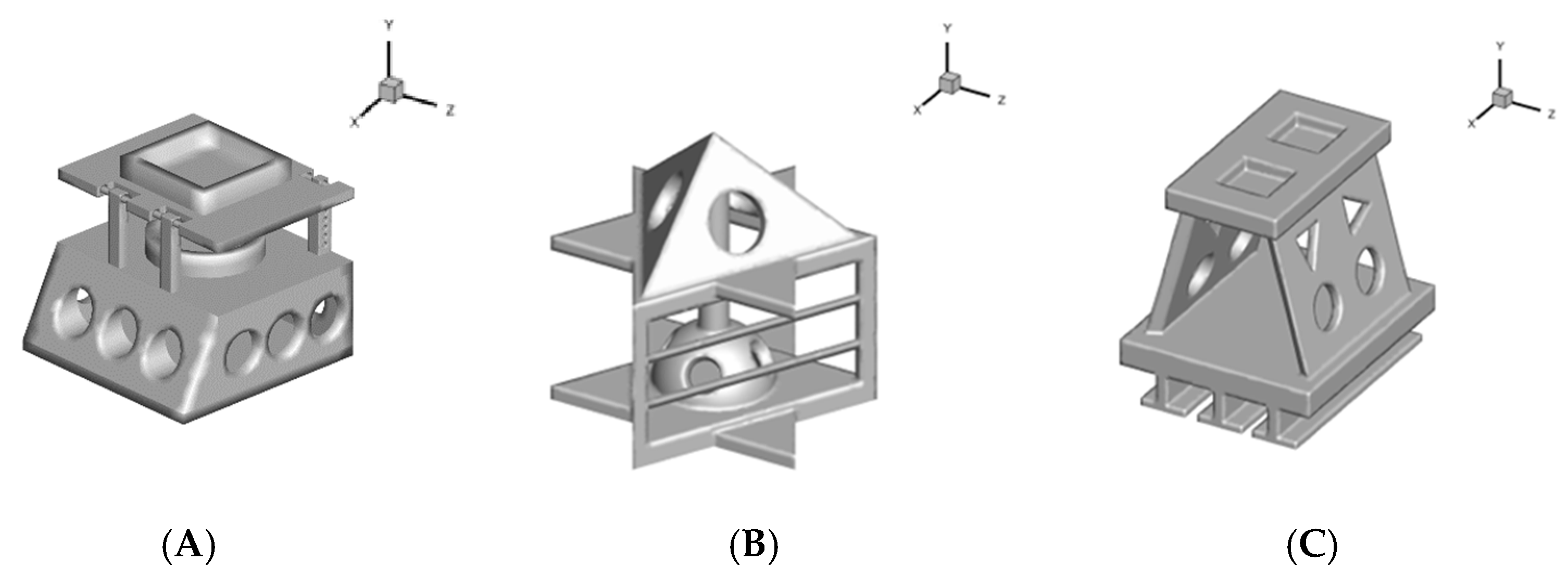
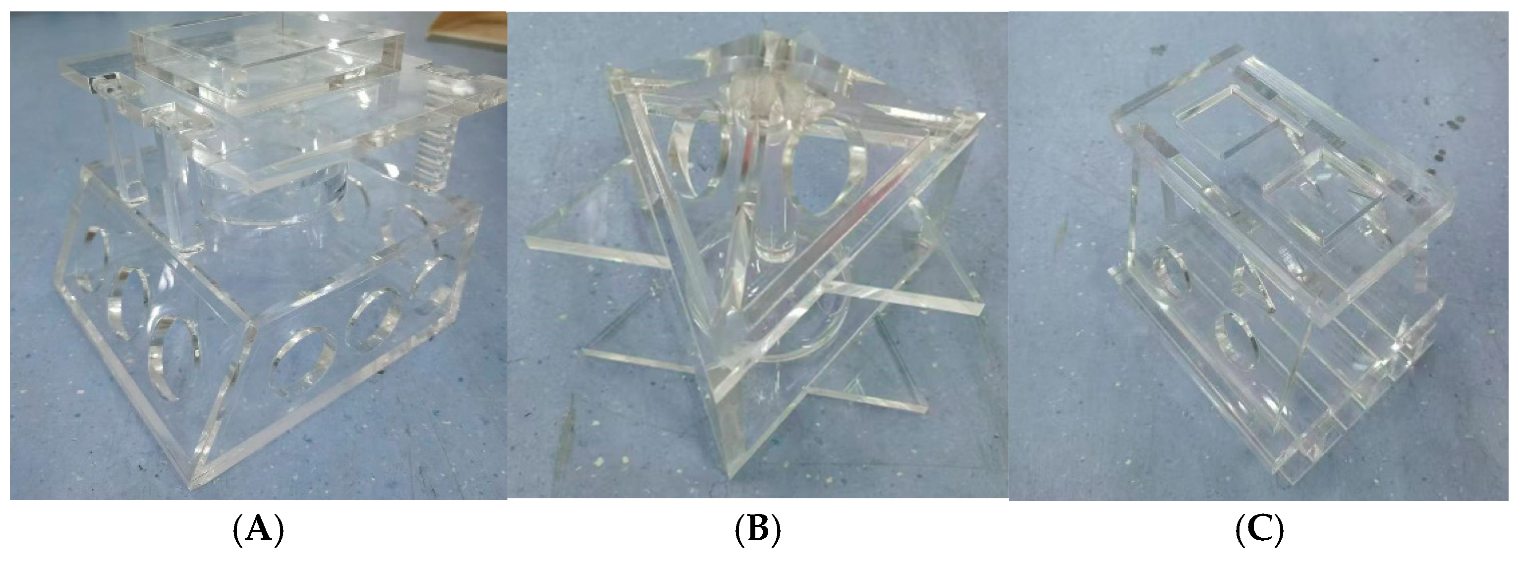
2.1. Reef Model

The simulation model with Solidwork designed three kinds of fish reefs, such as in Figure 1, material is reinforced concrete (Shanghai Ocean University, Shanghai, China), the size of the reef model A is 3 m (L) × 3 m (W) × 3 m (H), mainly for juvenile fish, the lower hollow side is open with holes to provide an ideal habitat for juvenile fish, and at the same time to simulate the shrimp in the natural environment of the habitat to provide food for the juvenile fish, the internal space allows juvenile fish to escape from the enemy. The upper and top layers are equipped with grooves to allow algae and shellfish to attach; Model B is in the shape of a hexagram, with dimensions of 2.7 m (L) × 2.7 m (W) × 2.25 m (H), targeting juvenile and sub-adult fish, which enter the sub-adult stage and increase in size and mobility. The structure of the frame can change the local water flow, making it easier for plankton to gather around the reef, and the gaps and channels between them can allow sub-adult fish to weave in and out of them and are sufficient to provide shelter space; Model C measures 3 m (L) × 2.7 m (W) × 3 m (H) and is mainly aimed at adult fish, which have a larger size and is fitted with a removable base at the bottom to prevent sinking. The reef has ample hollow space to provide a more expansive habitat for adult fish, and a groove is opened at the top to attach various algae and shellfish.

2.2. PIV Test

As shown in Figure 2, the test model was scaled down to a modeling size of 1:15, the material was Plexiglas (Shanghai Ocean University, Shanghai, China), and the model parameters are shown in

Table 1. Model parameters.

Type	Dimensions/mm (L × W × H)	Material
A	200 × 200 × 200	plexiglass
B	180 × 180 × 150
C	200 × 180 × 200

.

The flume test was carried out in a hydrodynamic circulation tank, as shown in Figure 3. The size of the flume test section is 200 cm × 80 cm × 70 cm (L × W × H), and the maximum flow rate can be up to 1 m/s. It is also equipped with a data acquisition instrument, a high-speed camera, a laser, and a PIV particle velocimeter. The fish reef model is fixed in the test section. The origin is located in the center of the reef body bottom point, along the current direction for the x-axis positive (flow direction), vertical current direction up for the y-axis positive (lateral), to establish a three-dimensional coordinate system. The flow field in the x-y center-axis plane of the reef was measured using PIV during the test.

(1)

The fish reef model was placed 0°, 15°, 30° and 45° to the flow angle, the target flow velocity was set, and the flow-making device was turned on;

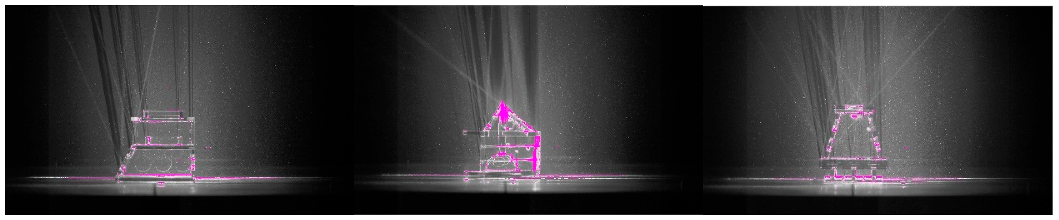
(2)

After the flow velocity was stabilized, a high-speed camera was used to take pictures and collect image data, see Figure 4.

(3)

The obtained particle images were first imported into PIV lab (2022) for processing, and the transient flow field map was obtained by selecting the image region to be analyzed for image correction, image analysis, error vector rejection, and data smoothing.

(4)

The data processed by PIVlab were imported into Tecplot (2022 R1) software for further detailed processing and analysis.

In the test process, the water depth is 60 cm constant, according to the prototype hydrological parameter conversion. It is more convenient to study the change rule of the flow field to choose 0.3 m/s, 0.4 m/s, and 0.5 m/s: three kinds of flow velocity gradients. As shown in Figure 5, 100 mm after the reef on the central axis, every 30 mm from the bottom of a measuring point, a total of 10 measuring points, from bottom to top are measurement points 1, 2,……9, 10—three kinds of fish reefs under different conditions of the flow velocity values for comparison—to analyze the flow field after the reef.

2.3. Numerical Simulation Methods

2.3.1. Governing Equations

In this paper, we adopt the RNG k-ε turbulence model, in which the basic idea is to regard turbulence as a transport process driven by random forces, eliminate its small-scale eddies by spectral analysis, and merge their effects into vortex viscosity [28] compared with the standard k-ε turbulence model, the RNG k-ε turbulence model has the following characteristics. The most important feature of the RNG k-ε turbulence model is that

(1)

The rotational and cyclonic flow cases in the mean flow are taken into account by correcting the turbulent viscosity.

(2)

An additional coefficient C₁ is calculated in the ε equation, thus reflecting the time-averaged strain rate S_i,j of the main flow, such that the resulting term in the RNG k-ε model is not only related to the flow situation but also a function of the spatial coordinates in the same problem.

Thus, the RNG k-ε model can better handle flows with high strain rates and a significant degree of streamlined bending and respond better to transient flows and streamlined bending effects than the standard k-ε model. The k and ε equations for the RNG k-ε model are as follows:

$${\displaystyle \frac{\partial }{{\partial }_t}}\left(\rho k\right)+{\displaystyle \frac{\partial }{\partial x_i}}\left(\rho k{u}_i\right)={\displaystyle \frac{\partial }{\partial x_i}}\left({\alpha }_k{\mu }_{eff}{\displaystyle \frac{\partial k}{\partial x_i}}\right)+G_k-\rho \epsilon$$

(1)

$${\displaystyle \frac{\partial }{{\partial }_t}}\left(\rho \epsilon \right)+{\displaystyle \frac{\partial }{\partial x_i}}\left(\rho \epsilon u_i\right)={\displaystyle \frac{\partial }{\partial x_i}}\left({\alpha }_{\epsilon }{\mu }_{eff}{\displaystyle \frac{\partial \epsilon }{\partial x_i}}\right)+C_{1\epsilon }{\displaystyle \frac{\epsilon }{k}}{G}_k-C_{2\epsilon }{\displaystyle \frac{{\epsilon }^2}{k}}-R_{\epsilon }$$

(2)

where $\rho$: Fluid density (kg/m³); $x_i$: a spatial coordinate variable in the Cartesian coordinate system, where i is a dummy scale (taking the values 1, 2, 3)$;u_i$: Time-averaged velocity components (m/s); ${\mu }_{eff}=\mu +{\mu }_t$: Effective viscosity coefficient, where μ is the kinetic viscosity, Pas and ${\mu }_t=\rho {\complement }_{\mu }{\displaystyle \frac{k^2}{\epsilon }}$ is the turbulent viscosity (Pa·s); $G_k={\mu }_t\left({\displaystyle \frac{\partial u_i}{\partial x_j}}+{\displaystyle \frac{\partial u_j}{\partial x_i}}\right){\displaystyle \frac{\partial u_i}{\partial x_j}}$: Turbulent kinetic energy production term, representing energy generation due to mean velocity gradients; ${\alpha }_k$,${\alpha }_{\epsilon }$: Turbulent Prandtl numbers for k and ε, set to 1.39 and 1.39, respectively; $C_{1\epsilon }=1.42$, $C_{2\epsilon }=1.68$ Empirical constants; $R_{\epsilon }={\displaystyle \frac{{\complement }_{\mu }{\eta }^3\left(1-\eta /{\eta }_0\right)}{1+\beta {\eta }^3}}{\displaystyle \frac{{\epsilon }^2}{k}}$ RNG-specific additional term, where $\eta =\sqrt{2S_{i,j}{S}_{i,j}}{\displaystyle \frac{k}{\epsilon }}$, ${\eta }_0=4.38$, and $\beta =0.012$.

The basic equations of the numerical model of artificial reef hydrodynamics are the continuum equations with the N-S equations for viscous incompressible fluids without considering the variation in the fluid density:

$${\displaystyle \frac{\partial \rho }{\partial t}}+{\displaystyle \frac{\partial }{\partial X_i}}\left(\rho {\overline{u}}_i\right)=0$$

(3)

$${\displaystyle \frac{\partial }{\partial t}}\left(\rho {\overline{u}}_i\right)+{\displaystyle \frac{\partial }{\partial X_i}}\left(\rho {\overline{u}}_i{\overline{u}}_j\right)=-{\displaystyle \frac{\partial \overline{p}}{\partial X_i}}+{\displaystyle \frac{\partial }{\partial X_j}}\left(\mu {\displaystyle \frac{\partial {\overline{u}}_i}{\partial X_j}}\right)-{\displaystyle \frac{\partial {\tau }_{ij}}{\partial X_j}}$$

(4)

where ${\overline{u}}_i,{\overline{u}}_j(i,j=\mathrm{1,2},3,i\ne j)$. The average flow rate of X, Y, and Z directions under the spatial coordinate system after filtration is m/s. $\overline{p}$ is the average pressure after filtration, Pa; μ is the kinetic viscosity, Pas; ${\tau }_{ij}$ is the sub-lattice stress, which is expressed as follows: ${\tau }_{ij}=\rho \stackrel{——}{{\mu }_i{u}_j}-\rho {\overline{u}}_i{\overline{u}}_j.X_i$ is the spatial coordinate variable, which is the tensor notation in a Cartesian coordinate system. Finally, i is a dummy (value of 1, 2, 3) corresponding to the direction of the (x, y, z) coordinates in three-dimensional space.

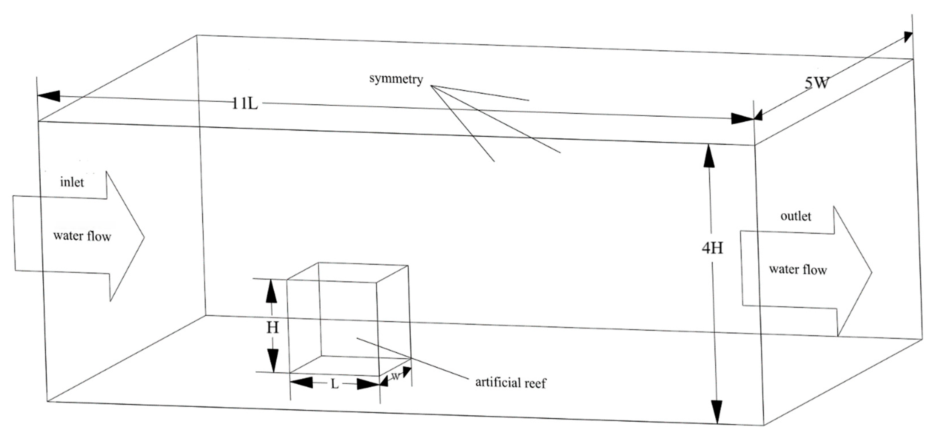
2.3.2. Computational Domain and Boundary Conditions

The computational domain of the flow field in this study includes an inlet boundary, outlet boundary, symmetry boundary, and wall boundary, and the computational domain is set to be 3 times the reef length in front of the reef, 7 times the reef length in the back, 5 times the reef width in width, and 3 times the maximum height of the reef in height, as shown in Figure 6.

The following settings are provided for the boundary conditions:

(1)

The inlet boundary condition is a velocity inlet. The corresponding incoming velocity is set, and the turbulence intensity and turbulent viscosity ratio on the boundary are calculated and given.

(2)

The outlet boundary is a pressure outlet.

(3)

The bottom surface of the computational domain and the surface of the artificial reef body are set as wall boundary conditions, the side walls are symmetric, and the standard wall boundary parameters of static no-slip are used.

Ansys Fluent Software (2022 R1) is used. In the simulation, the fluid density is set as the typical density of seawater 1024 kg/m³, and the second interpolation (QUICK) approximation is chosen for spatial discretization; the equations are iterated to the steady state by SIMPLEC for velocity–pressure correction; it is assumed that the residuals are lower than 10⁻⁵ when convergence is achieved. The current velocity in the sea area of South Sulawesi Province, Indonesia, is in the range of 0.1–0.5 m/s. Considering the influence of storm surge and extreme weather, the current velocity may increase to make the experimental results more obvious and contrasting, so the experimental incoming current velocity is selected as five velocities of 0.2 m/s, 0.4 m/s, 0.6 m/s, 0.8 m/s, and 1.0 m/s. The angle of the reef placement and the sea current may also affect the current field of the three different reefs’ flow fields; therefore, the four current-facing angles of 0°, 15°, 30°, and 45° were selected to investigate the effects of different flow velocities and angles on the flow fields of three different reefs.

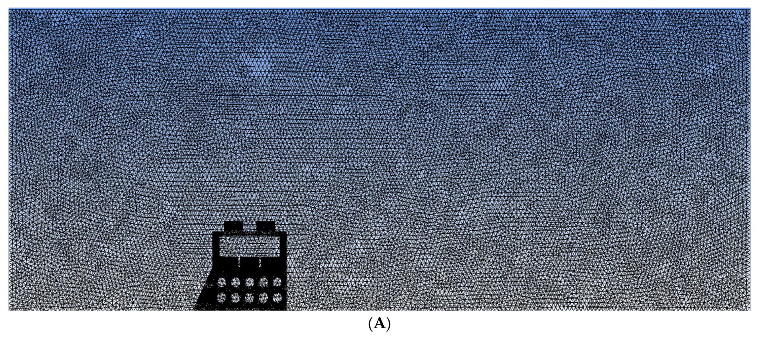
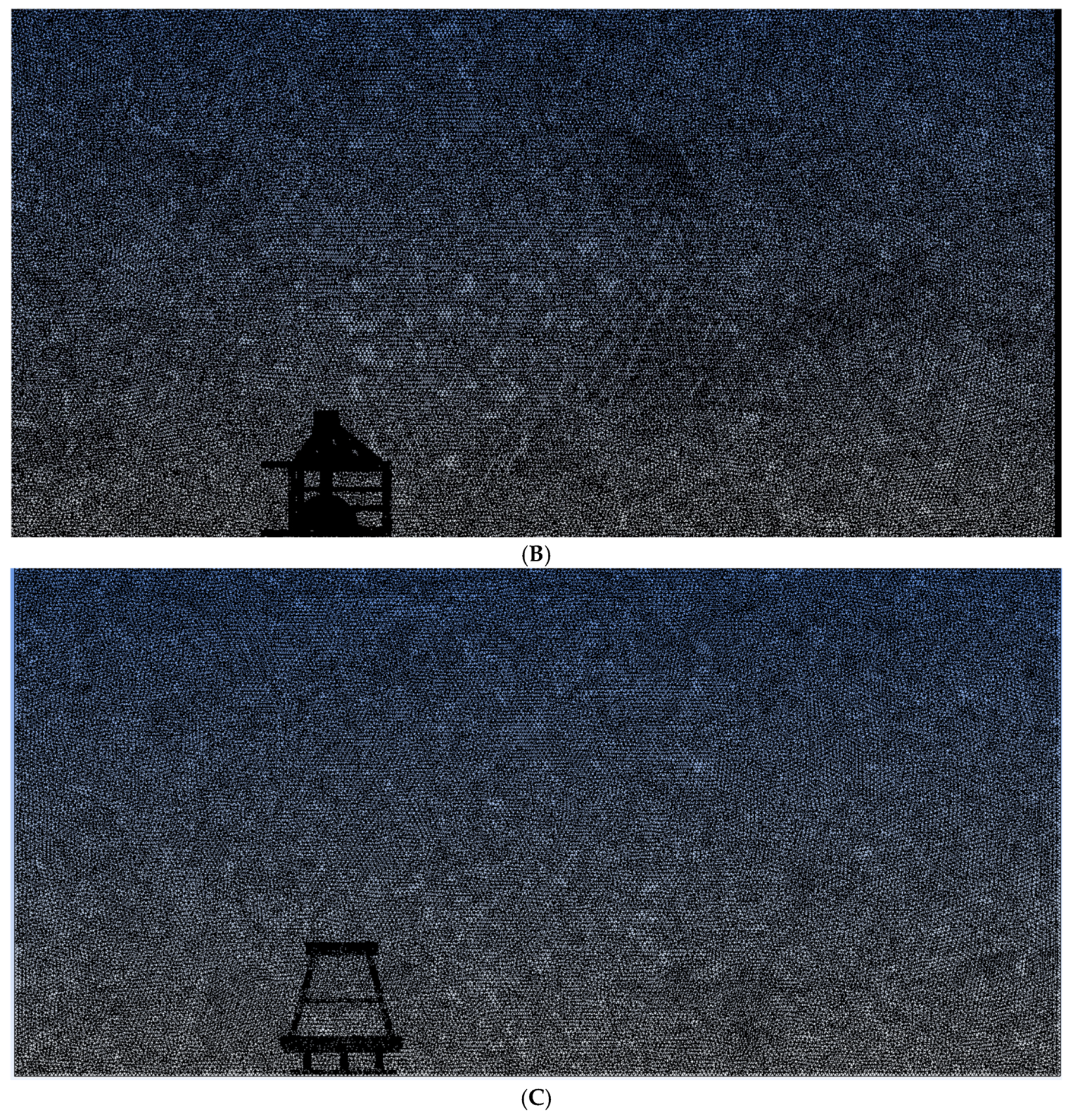
2.3.3. Meshing

Grids are divided to consider the accuracy of computation on the one hand and the efficiency of calculation on the other. Currently, grids can be roughly divided into two categories: structured grids and unstructured grids. As shown in

Table 2. Structured vs. unstructured grid characteristics.

	Structured Grid	Unstructured Grid
Advantages	Fast generation, high generation quality, and simple structure	Wide range of applications and simple generation
Disadvantages	Limited scope of application; only for regular shapes	Higher requirements for hardness and precision

, the respective advantages and disadvantages of structured and unstructured grids are listed [22].

In order to ensure that the simulation results effectively enhance calculation speed, we analyze symmetry based on the reef and computational domain characteristics, which are fully symmetrical. We assume the coordinate origin is at the center of the reef’s bottom surface, with the incoming flow direction aligned with the X-axis. The Y-axis represents the vertical direction, and Z = 0 in the pendant plane (XOY plane) serves as the central pendant plane of this study. As in Figure 7, the simulation model of the reef was created using Solidworks(2022) software and imported into the computational domain established by the ANSYS Workbench Mesh module(2022 R1). The area is meshed with tetrahedral unstructured mesh, the size of the flow field area is 0.1 m, the surface of the fish reef ranges from 0.045 to 0.09 m in size as required, the growth rate is 1.1, and the number of meshes of the fish reef model is in the range of 1 × 10⁷ to 1 × 10⁸.

2.3.4. Selection of Indicators for the Flow Field Region

The scaled index of the flow field effect of artificial reefs is an evaluation factor used to indicate the impact of the flow field of artificial reefs. The effect of the flow field is mainly generated by the upwelling on the facing surface and the back eddy on the back surface. When the flow velocity reaches a specific value, the corresponding flow field movement will produce the corresponding functional effects. Hence, the speed index is the selected standard of the upwelling and back eddy area. For this reason, the upwelling zone was chosen as the velocity region where the vertical flow velocity at the front of the reef was more incredible than 10% of the incoming flow velocity. The back eddy zone was the velocity region where the absolute value of the incoming flow velocity at the back of the unit reef was less than 80% of the incoming flow velocity [29].

3. Results

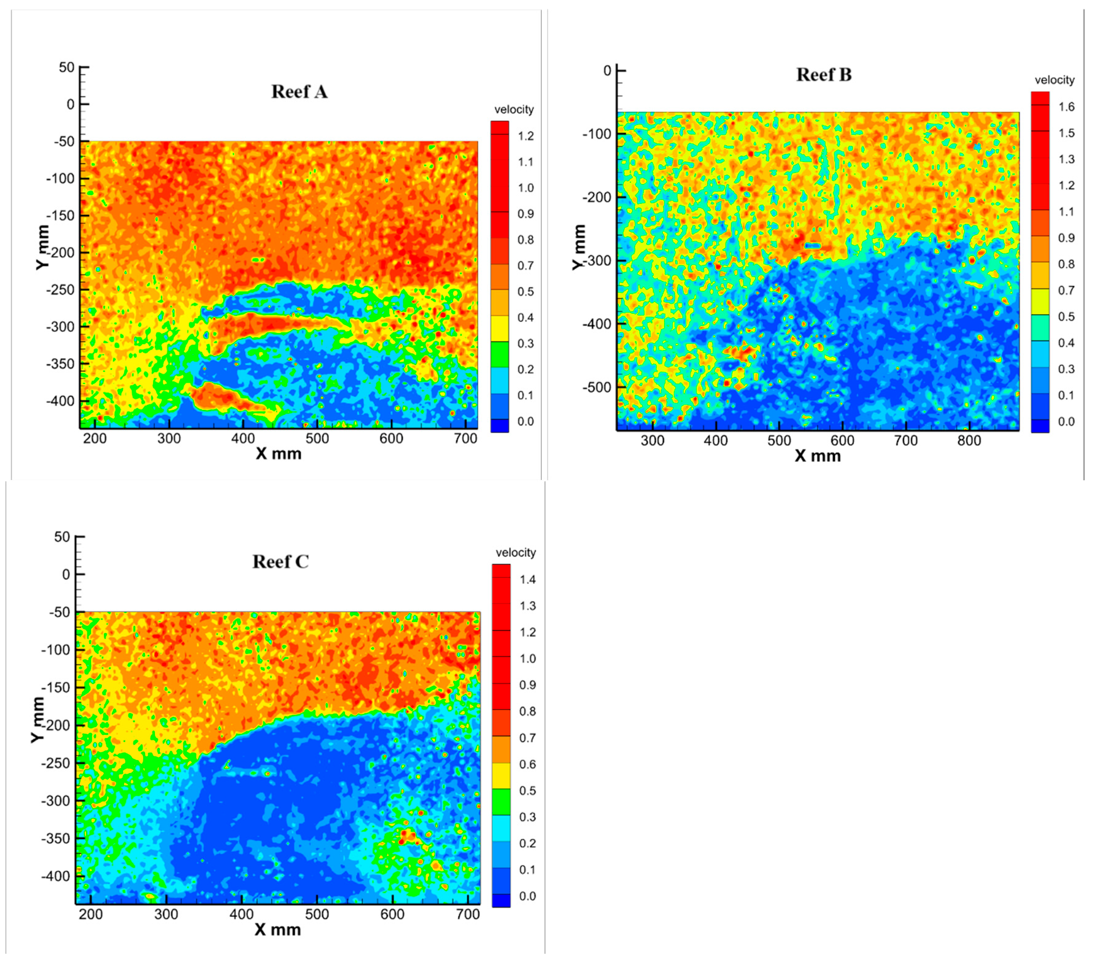
3.1. Test Results

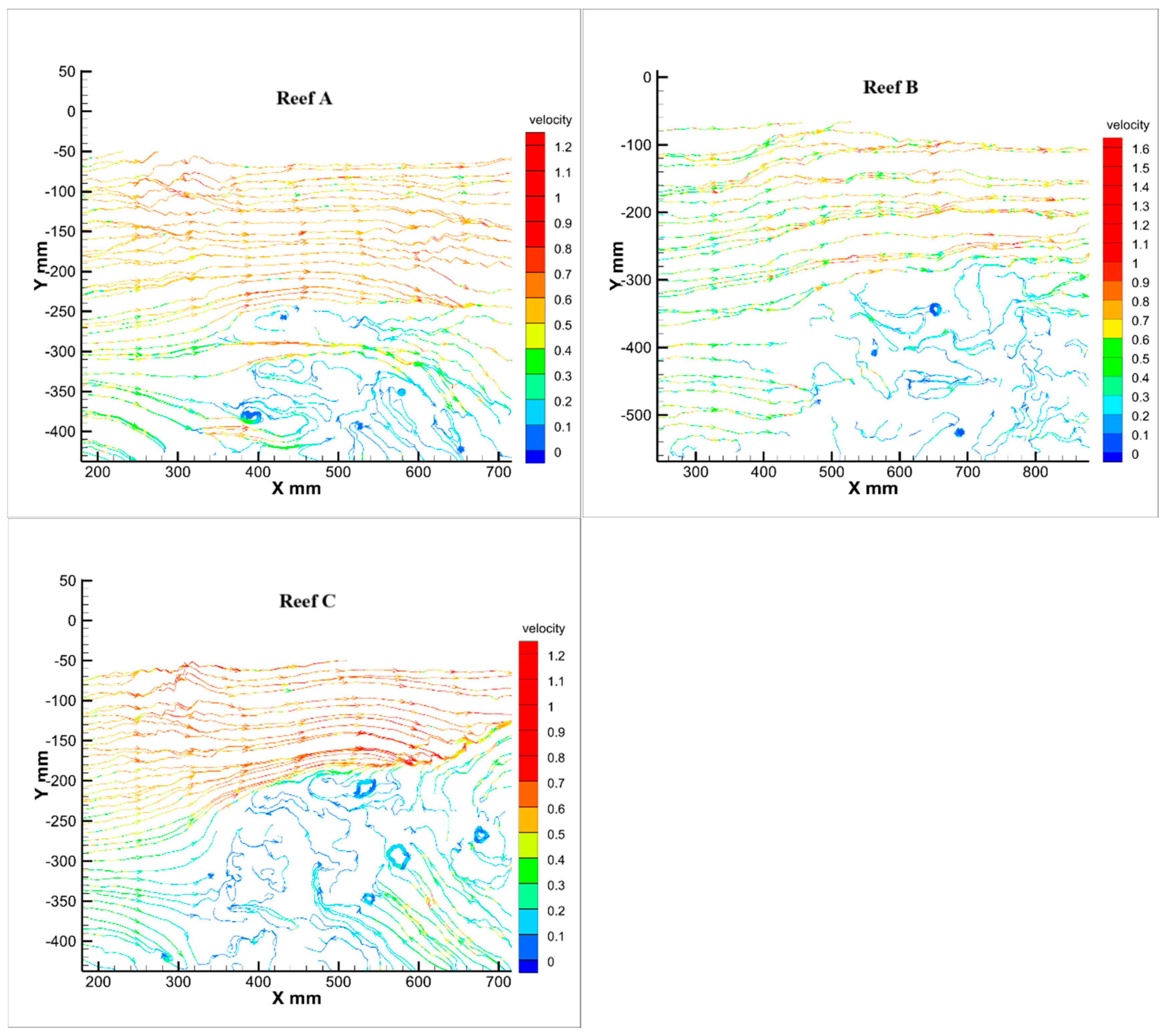
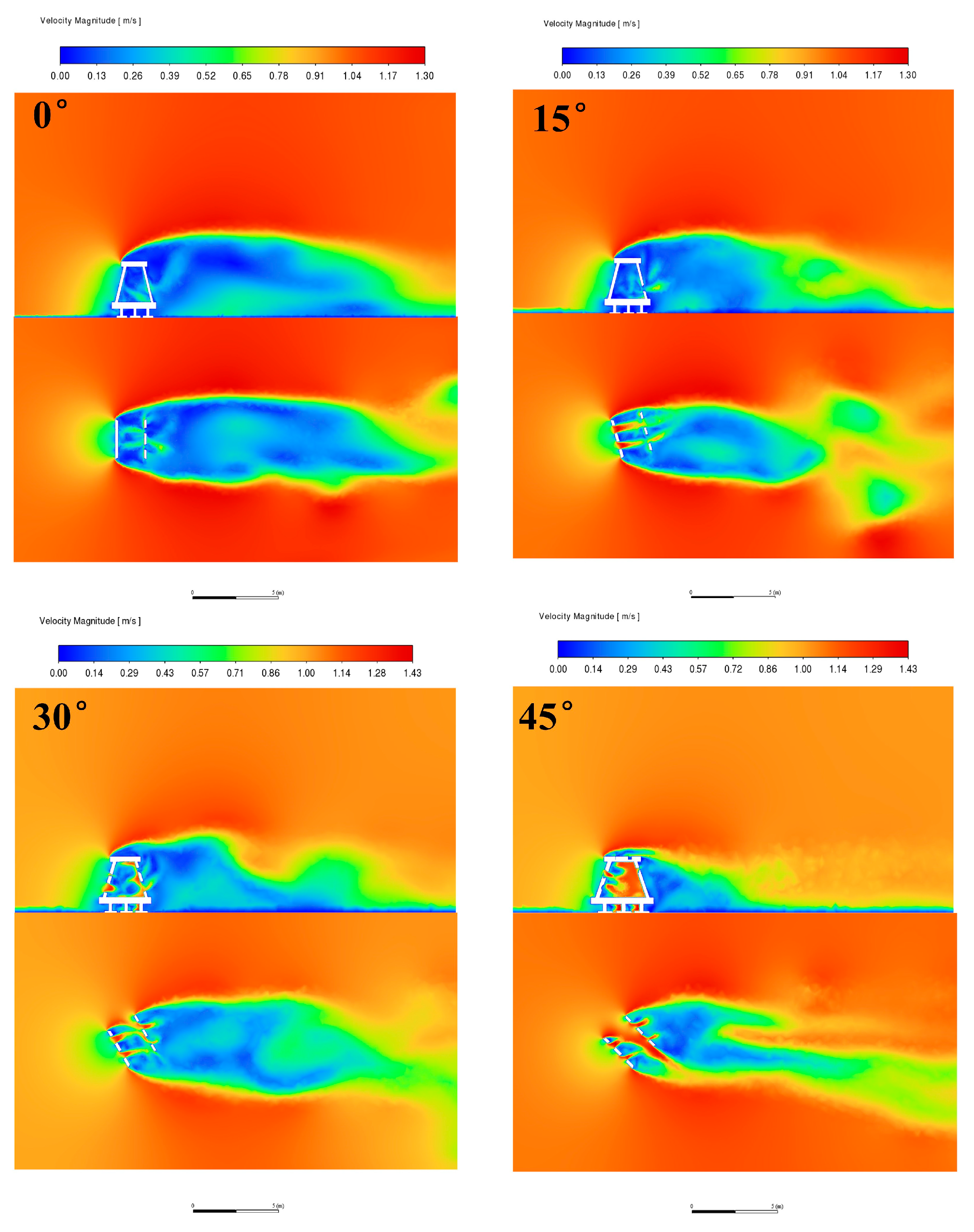
3.1.1. Characterization of Flow Patterns in the Mid-Axial Plane

As shown in Figure 8 and Figure 9, the flow conditions of the axial surface particles in the three types of artificial reefs are compared when the angle of the headward current is 0° and v = 0.5 m/s. From the figure, it can be seen that all three types of artificial reefs form a specific scale of upwelling above them. The upwelling areas of A and C are more extensive, and a small portion of the slow flow area is generated within 50 mm above the reef. Among them, the cavity structure of Reef A demonstrates a noticeable gap pipe flow effect inside the reef.

Meanwhile, the upwelling area of Reef B is smaller, and the inclination angle of the flow-facing surface is smaller. On the contrary, Reefs B and C have larger back eddy areas, and Reef A reduces the scale of the back eddy behind the reef due to its internal cavity structure. Velocity vector plots show that all three types of reefs have significant eddy generation behind the reefs. In the wake behind Reef C, a part of the current touches the bottom to form an upwelling with an increased velocity. There is also a significant acceleration of the current at the inner void of Reef A and small areas of eddy disturbance at and around the inner structure of Reefs B and C.

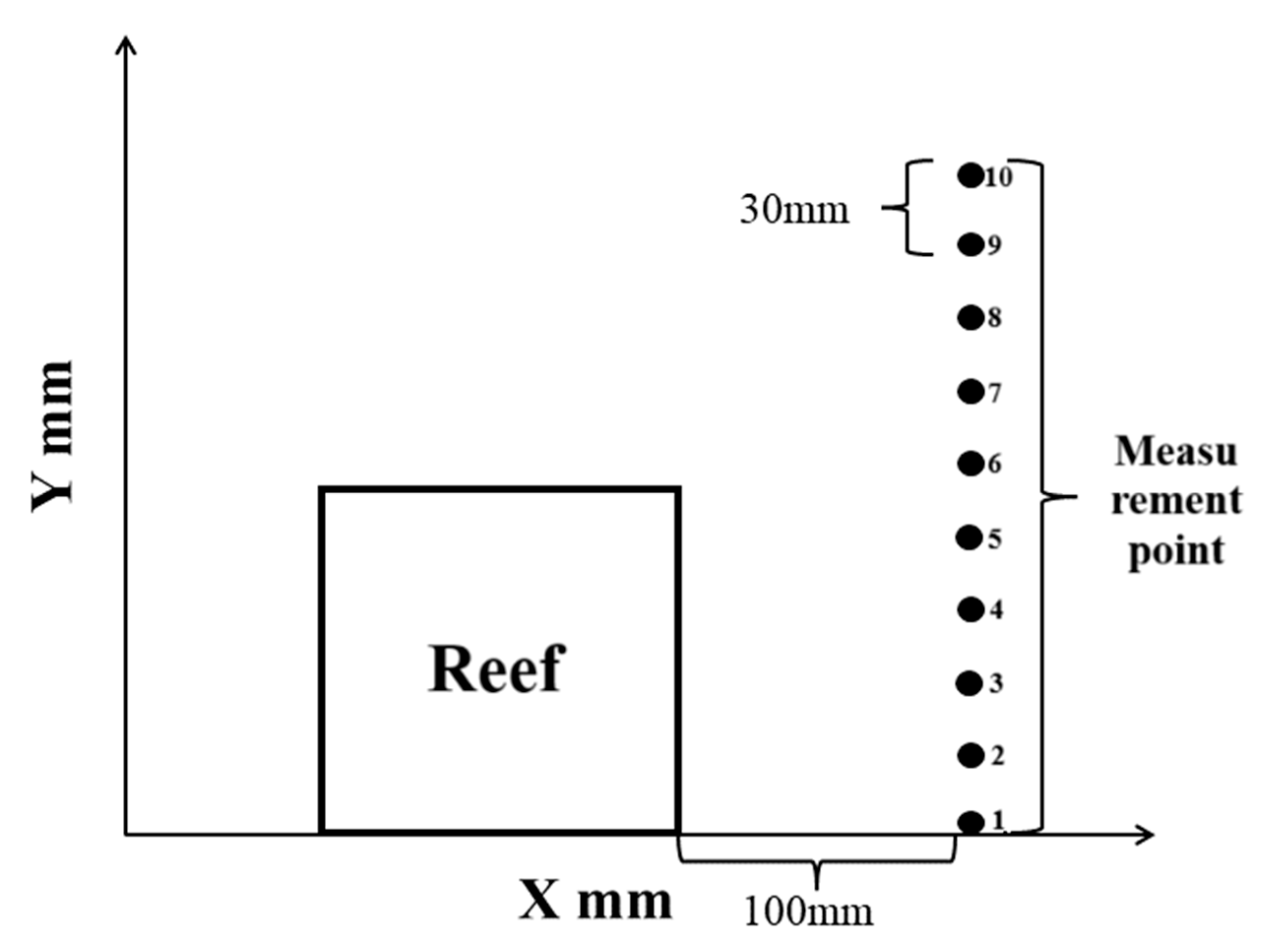
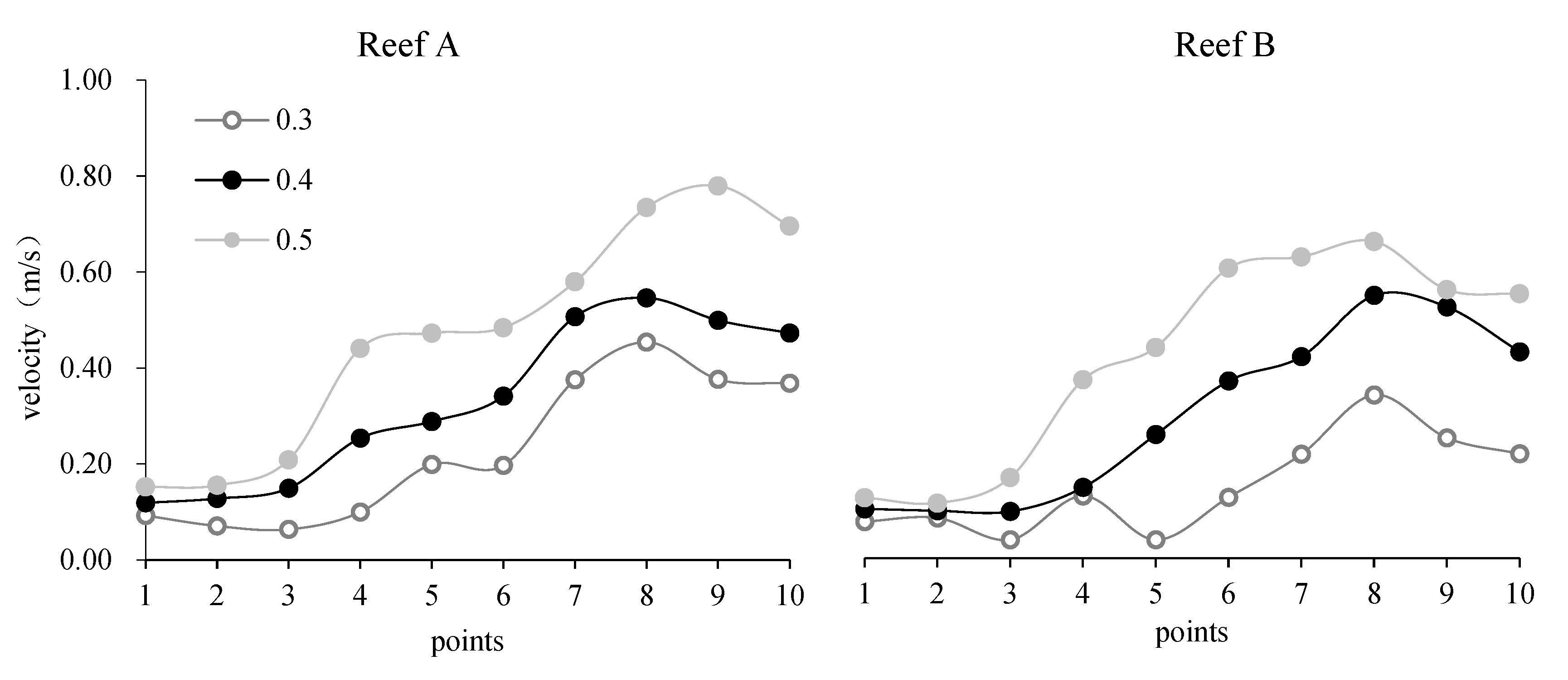
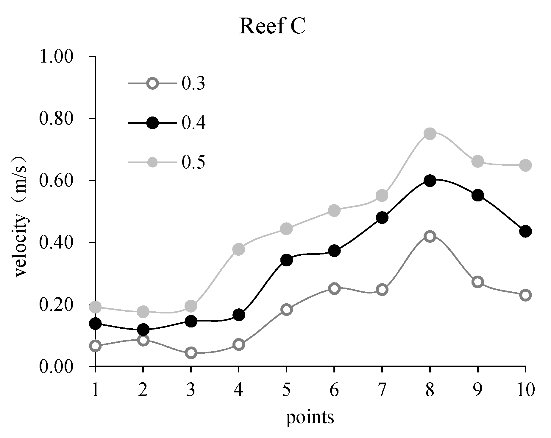
3.1.2. Point Velocity Results

As shown in Figure 10, the flow velocities at each reef are compared and analyzed at three headwater velocities at a 0° headwater angle. The figure shows that with the increase in the headward current velocity, the flow velocity of all the measurement points of the three types of Reefs, A, B, and C, increases, of which the first four measurement points show minor changes, i.e., the flow velocity in the back eddy area behind the reefs demonstrates minor changes. After measurement point 6, i.e., the upwelling area has significant changes. Overall, the velocity of the three types of reefs behind Reefs A, B, and C tends to increase first and then decrease.

3.2. Numerical Results

3.2.1. Cross-Sectional Flow Characteristics

Figure 11, Figure 12 and Figure 13 compare the flow conditions in the axial plane (x = W/2) and cross-section (y = H/2) of the three artificial reefs, A, B, and C, for different incoming flow velocities at a headwater angle of 0°.

When the incoming flow meets the reef body, due to the water flow contacting the reef body’s headward surface, the ascending effect at the top of the reef produces a significant speed-up phenomenon and a certain amount of upwelling. In Reef A’s center cavity, the gap tube flow effect accelerated the flow velocity, reaching its maximum in the cavity’s flow field area, which includes a baffle groove, creating a slow flow area. When the water flow passes through the reef area, the flow velocity shows a significant slowdown due to the increased contact volume of the water flow with the flow field area, reflecting the hindering effect of the fish reef on the incoming flow and generating a backflow area behind the fish reef to form a back eddy flow area. Due to the fewer openings in Reef C, the area of the oncoming flow is relatively larger, showing a good obstruction effect and generating a good eddy effect behind the reef. The upwelling and back eddy areas are significantly larger than those of the remaining two groups of fish reefs. Reefs A, B, and C have more and larger open holes. Reef A has a more extended wake with the increase in velocity, the area of the back eddy has increased, and from the cross-section, it can be seen that there is a clear diversion of the flow after the flow passes through the back of the reef body. A fuzzy vortex is generated on both sides, and as the flow velocity increases, Reef B demonstrates an increased wake, accompanied by a rise in velocity. The Karman eddy behind the reef body demonstrates a desirable effect. The upwelling and back eddy area is significantly larger than the remaining two groups. The Karman vortex phenomenon behind the reef is more prominent, as Reef A’s upwelling and back eddy have a larger area than the remaining two reefs.

Figure 14, Figure 15 and Figure 16 compare the flow regimes in the axial plane (x = W/2) and cross-section (y = H/2) of the three artificial reefs, A, B, and C, at v = 1.0 m/s for different headwater angles.

Under different flow angles, the flow pattern inside the reef and the basin changes significantly due to the surface change. Reef A has a more obvious Karman vortex on the left side at 15°, and the larger the angle is, the more pronounced the diversion phenomenon. The wake becomes shorter, the area of the back eddy decreases, and the tube flow effect inside the reef disappears gradually. Reef B demonstrates the disappearance of the Karman vortex with the increase in the angle, the back eddy area decreases, and there is a tube flow phenomenon in the reef. Reef C also showed a decrease in the area of the back eddy as the angle increased, a divergence of the flow behind the reef at 45°, and a tube flow effect in the internal structure.

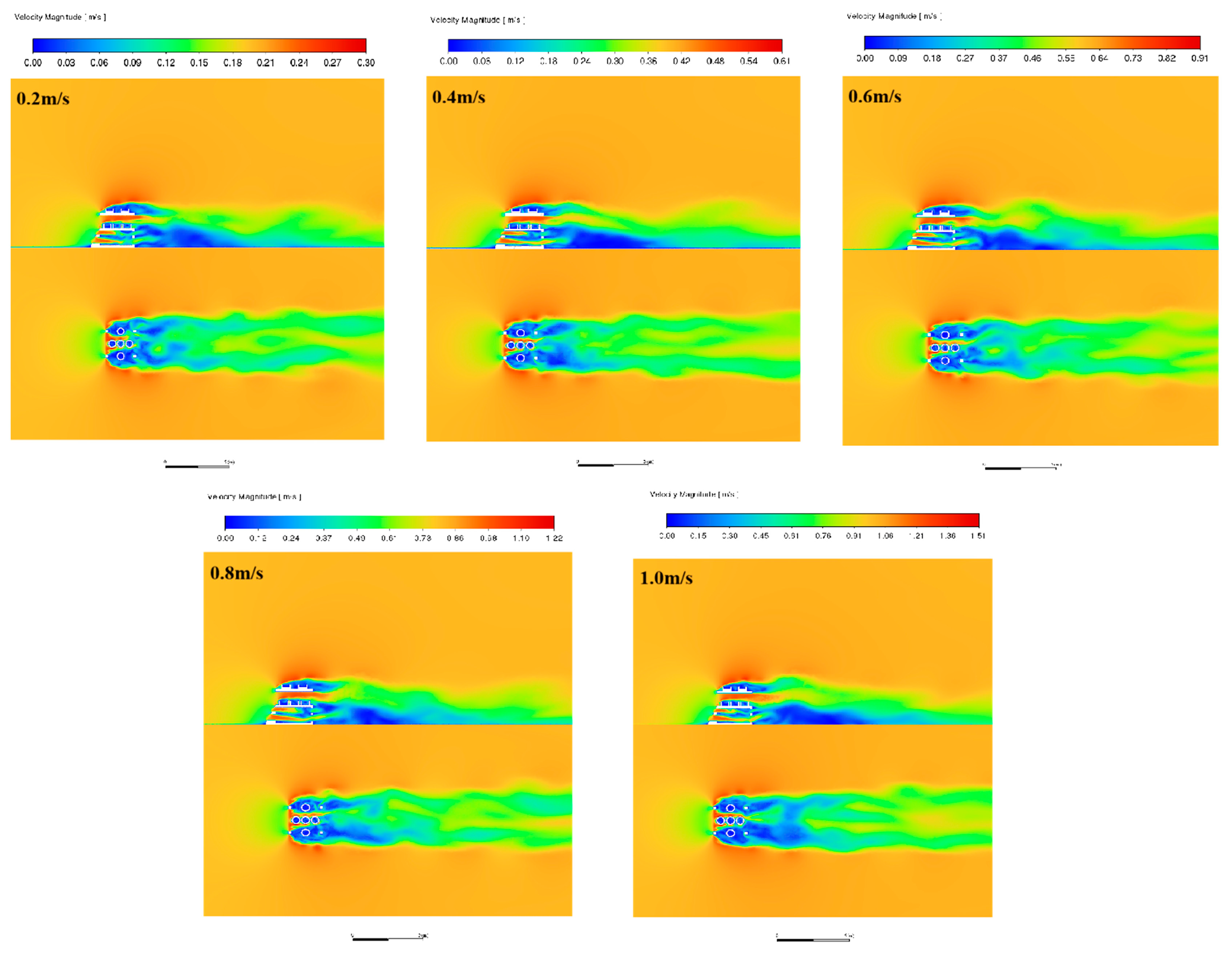
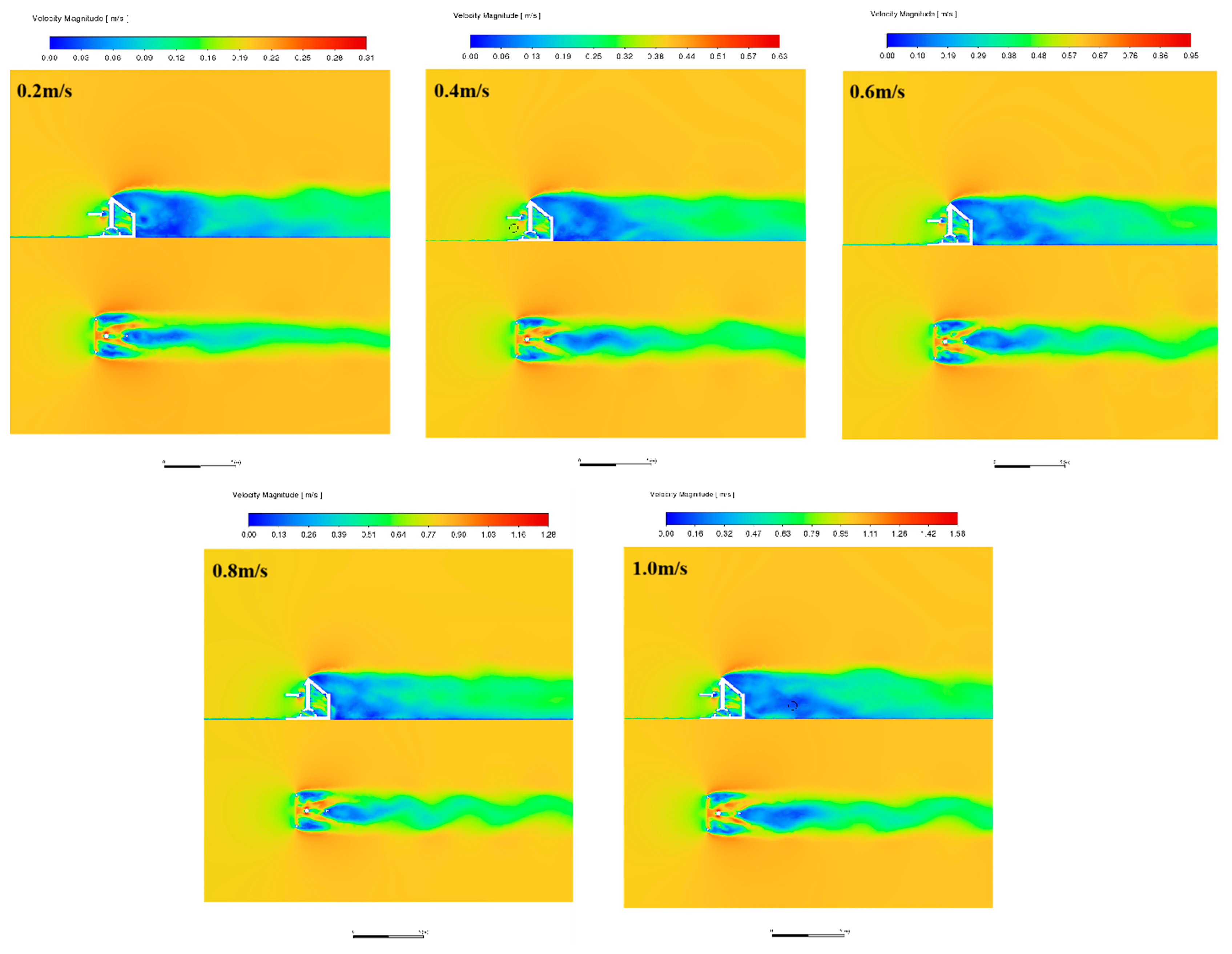
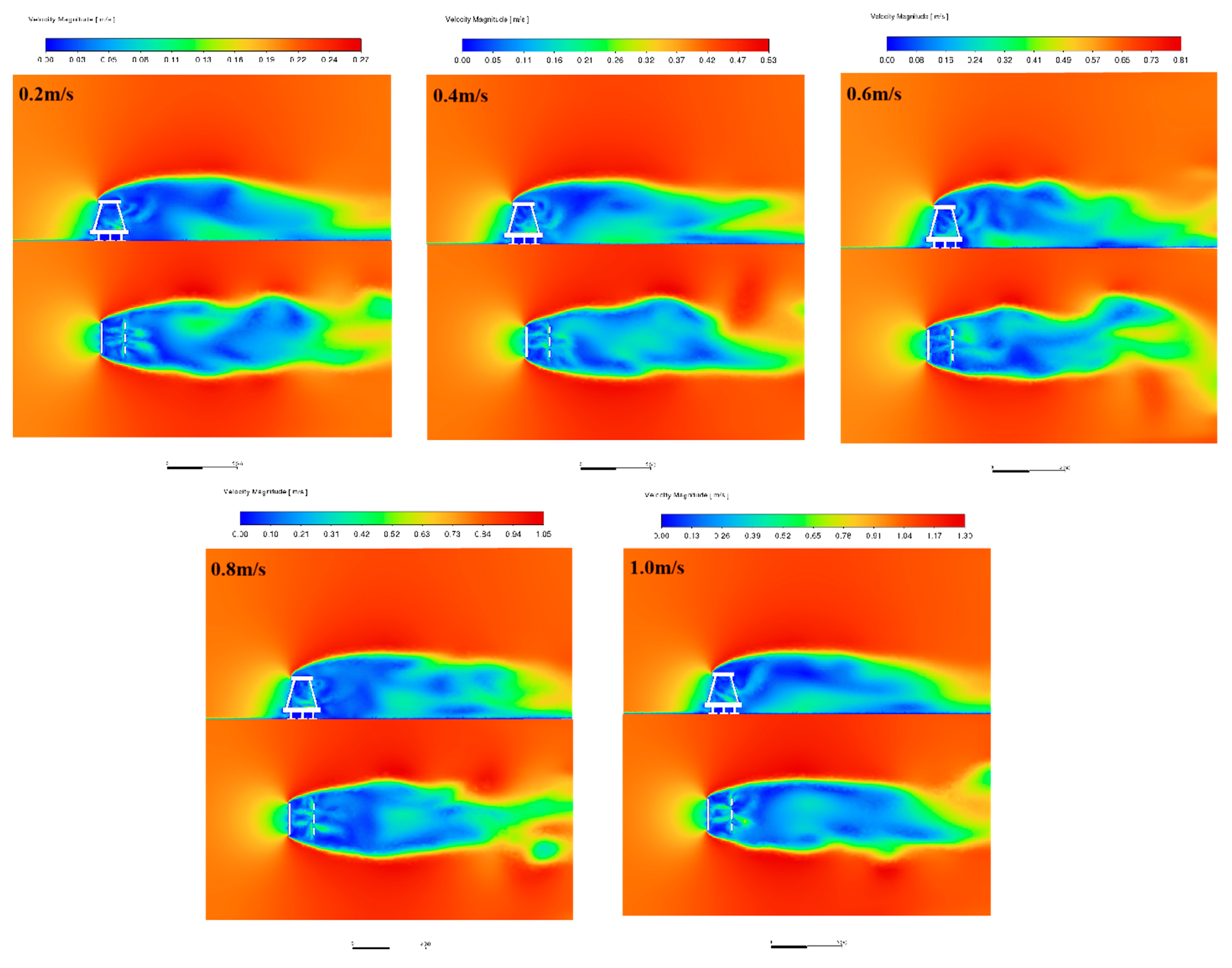
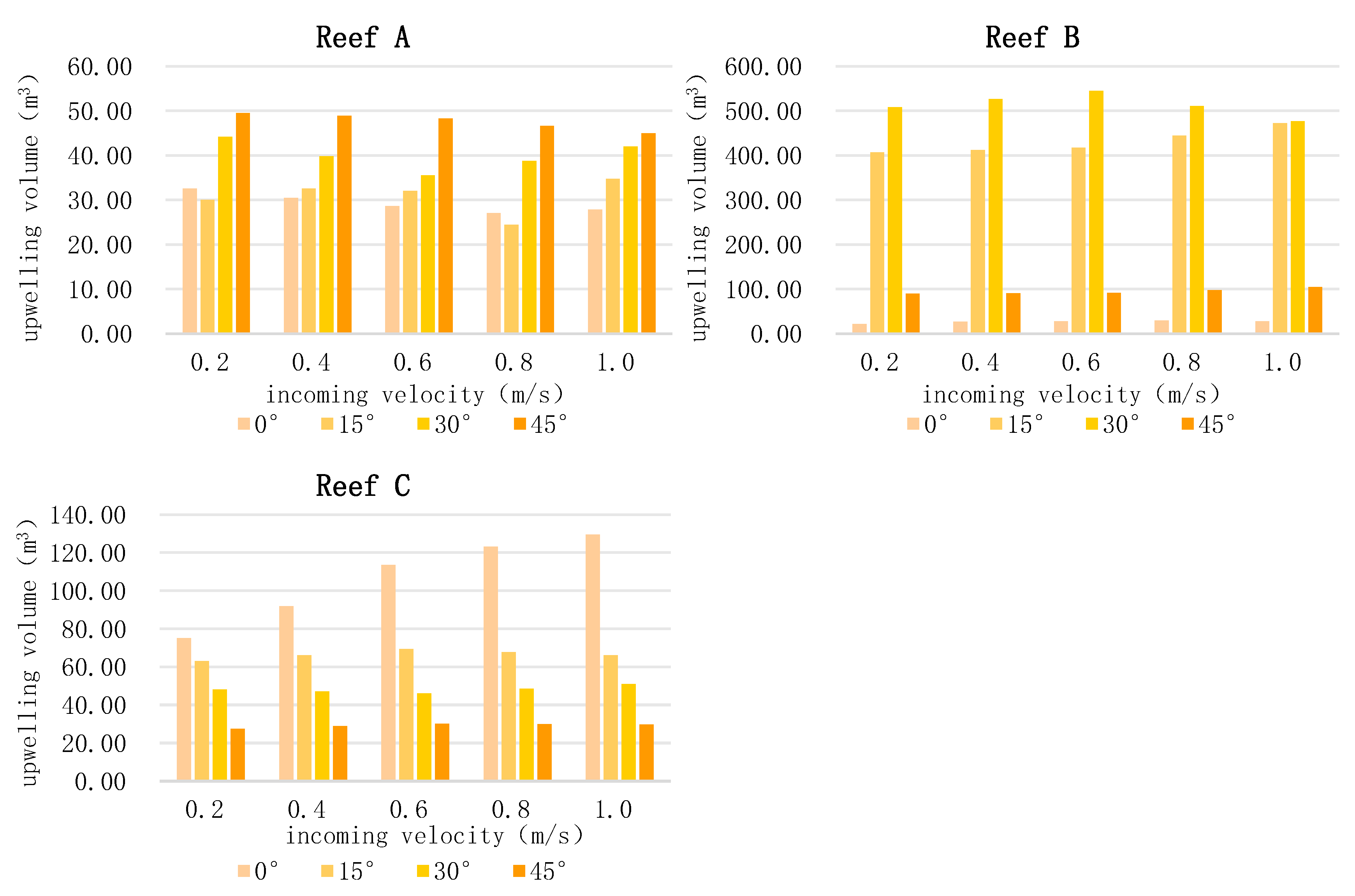
3.2.2. Volume Characteristics of the Flow Field for Different Incoming Velocities

As shown in Figure 17 on three different artificial reefs with varying angles of flow and changes in flow velocity and the impact on the upwelling, take the incoming velocities 0.2 m/s, 0.4 m/s, 0.6 m/s, 0.8 m/s, 1.0 m/s as a comparative analysis. For Reef A, the upwelling volume exhibits a slight decrease with increasing flow velocity at angles of 0° and 45°, though the variation remains statistically insignificant. At 30°, the volume initially decreases, reaches a minimum at v = 0.6 m/s and subsequently increases. In contrast, no significant change in upwelling volume is observed at 15°. The volume of the upwelling of fish in Reef B did not change significantly with velocity at 0° and 45° but increased with velocity at 15° then increased and then decreased at 30°, reaching a maximum at v = 0.6 m/s. The volume of the upwelling of fish Reef C increased with the velocity at 0° and 30°, respectively, and did not change significantly at the other angles.

As shown in Figure 18, for three different artificial reefs with varying angles of headwater, the back eddy is affected by the flow velocity change. For Reef A, the back-eddy volume increases with the velocity at angles of 15° and 45°, peaking at v = 0.8 m/s, for 15° and v = 0.6 m/s for 45°. At 0°, the volume initially decreases, reaches a minimum at v = 0.8 m/s, and subsequently increases. In contrast, at 30°, the volume exhibits a monotonic decrease with increasing velocity. Reef B decreases and then increases at 15°, reaches a minimum at v = 0.6 m/s, and there is no clear pattern of change with velocity at other angles. Reef C increases and then decreases at 0°, reaches a maximum at v = 0.6 m/s, and there is no clear pattern of change with velocity at other angles.

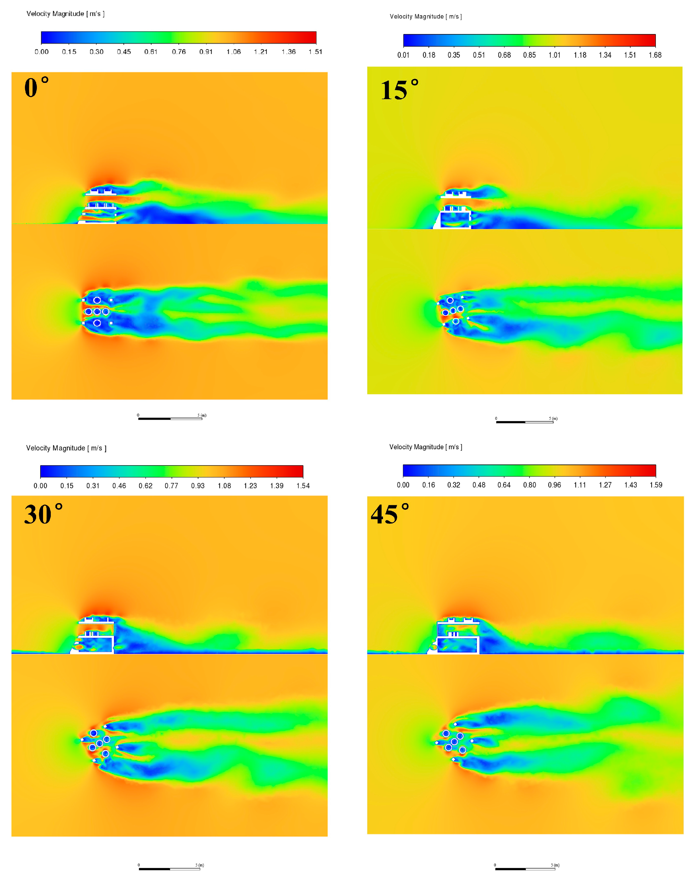
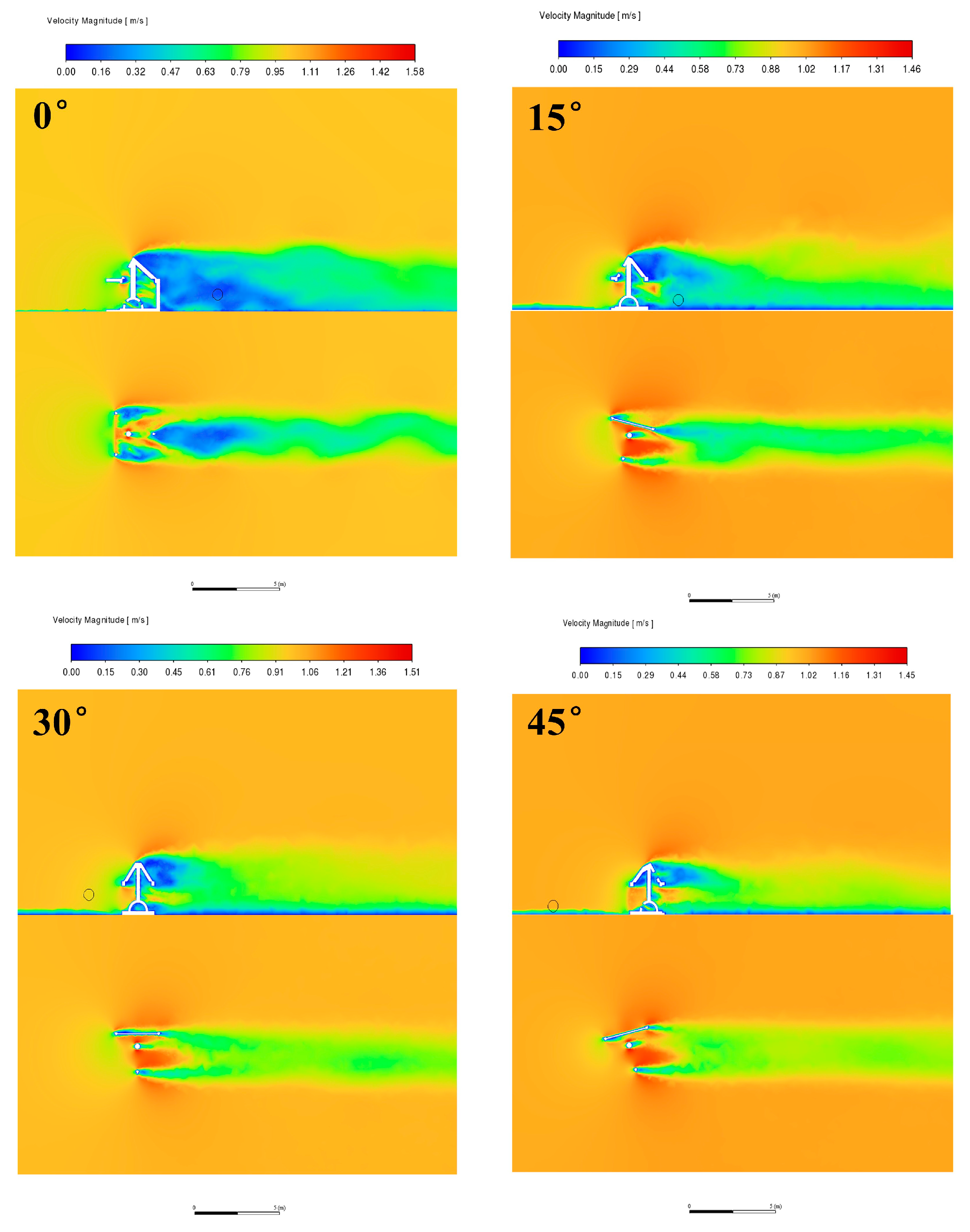
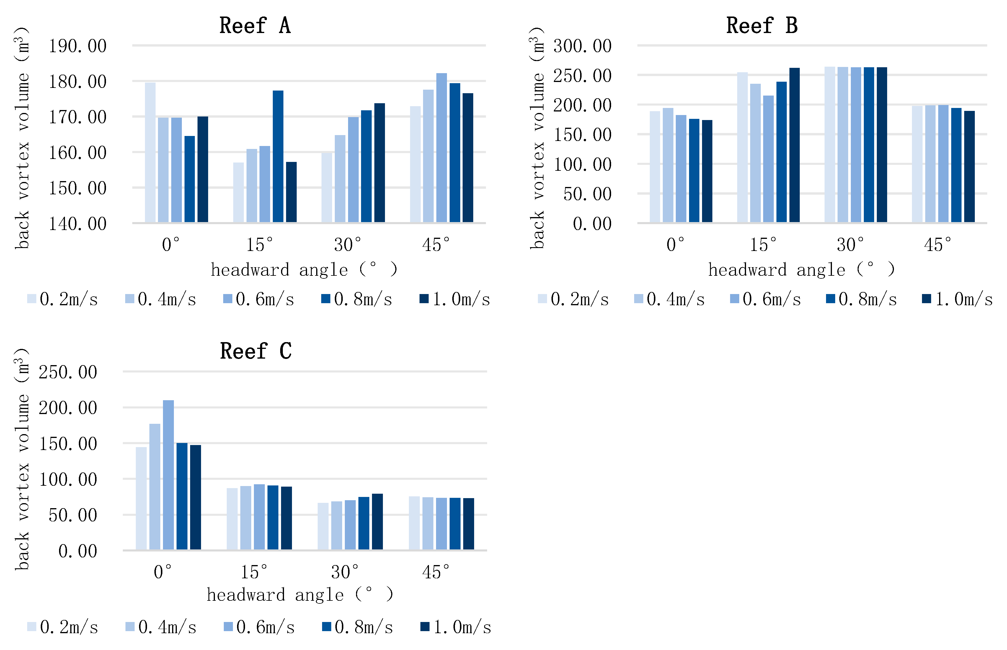
3.2.3. Volume Characteristics of the Flow Field for Different Flowing Angle

The effects of changes in the flow angle on the upwelling of three different artificial reefs at different incoming velocities are shown in Figure 19. Reef A’s upwelling volume decreases and then increases with the increase in the flow angle at v = 0.2 m/s and v = 0.8 m/s. Both are the smallest at 15° and increase with the flow angle increase at the other velocities. The volume of Reef B increases and then decreases with the increase in flow angle and is much larger than the rest of the angles at 15° and 30°, reaching the maximum at 30°. Reef C decreases with the increase in flow angle.

The effects of changes in the angle of flow on back eddy currents at different incoming velocities for three different artificial reefs are shown in Figure 20. The volume of back eddy currents on Reef A decreases and then increases with an increasing flow angle and is minimized at 15°. The volume of back eddy currents on Reef B increases and decreases with an increasing flow angle, reaching a maximum of 30°. The volume of back eddy currents on Reef C is much larger at 0° than at the other three angles, and the difference in volume of back eddy currents is relatively tiny in the different angles. Reef C has a much larger back eddy volume at 0° than the other three angles, and the difference in back eddy volume at other angles is slight.

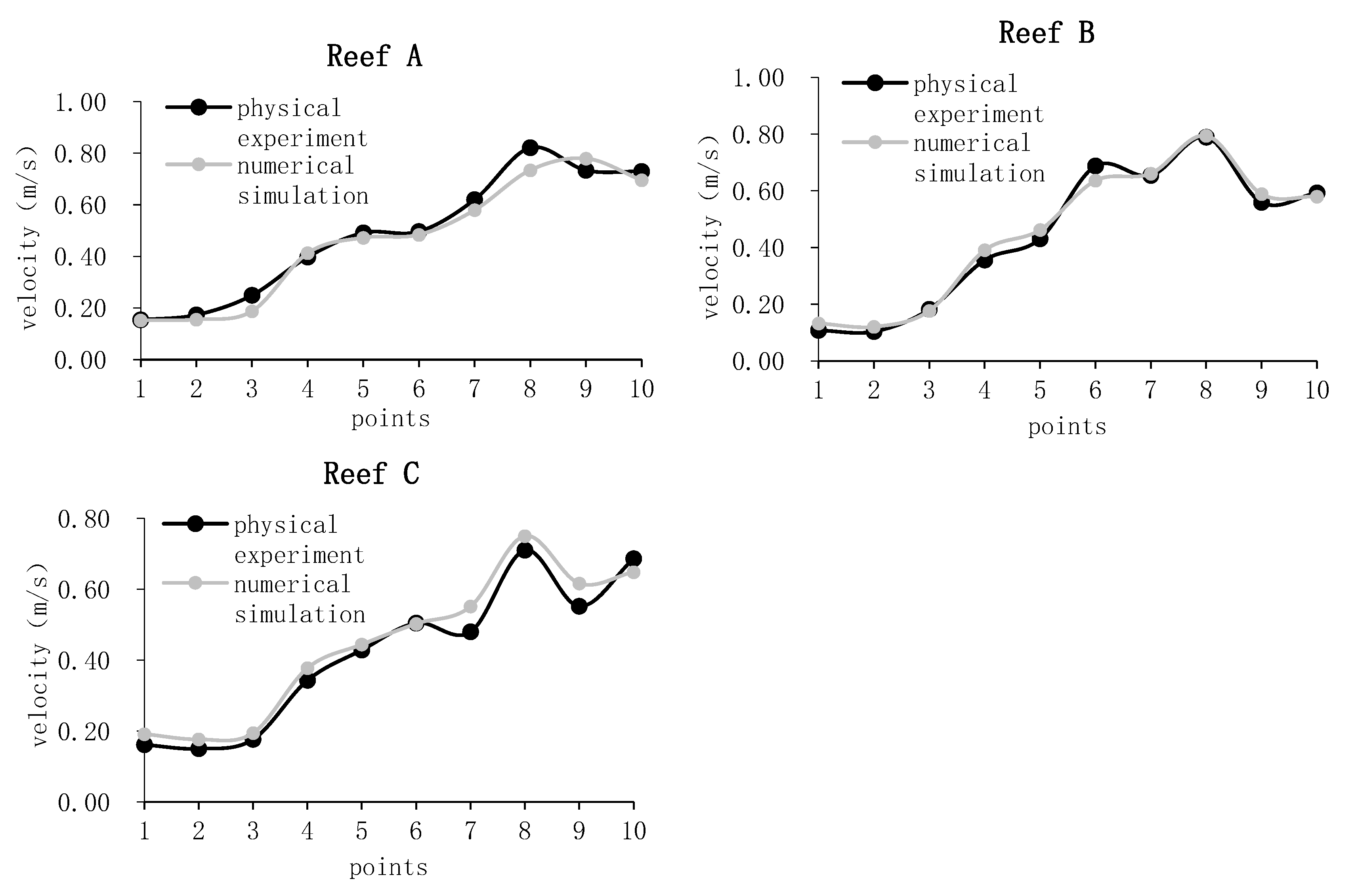
3.3. Validation of Results

Validation experiments were conducted using the control-point method with cross-sectional measurements. The computational domain and numerical model were scaled down by a factor of 15 following the same simulation methodology. Measurement points were aligned with their exact physical experimental locations to compare flow velocities between physical experiments and numerical simulations. The specific positions of these measurement points are illustrated in Figure 21. This setup was designed to analyze the back-eddy effects behind the reef and the trend of upper updrafts.

The comparison of flow velocity at different flow measurement points during the flume experiment and numerical simulation, as shown in Figure 20, indicates that the trends in velocity changes at the measurement points are consistent between the flume experiment and the pre-processed numerical simulation data. After calculation, the relative errors of the three types of reefs are 1.00~24.74%, 0.66~22.51%, 0.38~18.69%, and the average errors are 7.43%, 7.52%, and 9.86%.

4. Discussion

Incoming current velocity changes affect the upwelling and back-eddy volumes of different reefs. For example, the upwelling volume of the reef at 0° for Reef C shows a gradual increase with increasing incoming velocity [30]. This is because as the incoming current velocity increases, the impact force of the current on the reef increases accordingly, prompting more water to surge upwards and form a larger upwelling. However, the upwelling volume does not increase monotonically when the incoming velocity increases. The effect on the flow field is diminished when the reef reaches a certain height [31]. Reef A may decrease and then increase the volume of updraft at 30° operating conditions. When the incoming flow velocity is low, because the kinetic energy of the water flow is small, the obstruction effect of the fish reef on the water flow is relatively weak, and the formation of upwelling is more complicated. Given a gradual increase in the incoming flow velocity, the impeding effect of Reef A on the water flow at 30° is strong. Within a specific range, this impeding effect may lead to a decrease in the upwelling volume. When the incoming flow velocity continues to increase to a certain extent, the impact and shear forces of the water flow become strong enough to push more water flow upwards instead, thus increasing the upwelling volume again.

Meanwhile, the upwelling volume of the three types of reefs at certain angles did not change significantly when the incoming flow velocity changed due to the changes in the projected area of the structure and shape of these reefs at specific angles [32]. For example, Reef C is insensitive to changes in the incoming flow velocity due to the lack of change in the flow surface at 15°, 30°, and 45°. Alternatively, the flow field effect of the reef reaches a relatively stable state within a specific range of incoming flow velocities so that even if the incoming flow velocity changes, the upwelling volume does not change significantly.

The back eddy volume also shows different patterns with the change in the incoming flow velocity. For some conditions, the back eddy volume gradually increases with the increase in the incoming velocity. This is because an increase in the incoming flow velocity leads to an increase in the impact of the current on the reef, which makes the formation of back eddies behind the reef more pronounced [33]. The back eddy volume also decreases as the incoming velocity increases. This is because at higher incoming velocities, the kinetic energy of the current is higher, and the B-reef structure allows the current to bypass the reef quickly, which inhibits the formation of back eddies. Other reefs may show an increase and decrease in the volume of back eddies as the incoming velocity varies or may show no clear pattern of change.

Changes in the angle of the upwelling significantly affect the volume of upwelling and back eddy of the three artificial reefs, which shows a specific regular change [34]. When the angle of the headwater current changes, the relative direction of the current and the fish reef will also change, which leads to a change in the flow field around the fish reef. The different flow angles will change the obstruction and channelization of the reef to the water flow, affecting the formation of upwelling and back eddy.

For upwelling, the volume and strength of the flow change accordingly as the angle of flow increases. At certain flow angles, such as Reef A, the flow is more effective at impacting the reef at larger flow angles, resulting in a larger upwelling. When the current angle is small, e.g., Reef B at 0°, the current flows more gently over the reef, and the upwelling formation is relatively weak. When the flow angle is larger, the impact of the current on the reef increases, and the volume of upwelling increases. Continuing to improve the flow angle on the effects of the current on its reduced, the volume of upwelling decreases.

For back eddies, the formation of back eddies and diverging currents behind the reef may be more pronounced at some current angles, and the wake area behind the reef splits into multiple regions, with the total area of influence increasing and becoming more dispersed [35]. This disperses the rapids into multiple small eddies, slowing the current and allowing plankton to congregate. It also allows fish to reside in a relatively stable eddy area and reduces the risk of being swept away by the rapids, whereas at other current angles, the back eddies may be suppressed and reduced in size. Changes in the volume of back eddies at different current angles also vary among reefs depending on the shape and structural characteristics of the reef.

The shape of a fish reef determines factors, such as its current-facing area and cavity structure, which in turn significantly impacts the flow field effects of artificial reefs. Fish reefs with different shapes behave differently in currents, and shape factors can also constrain the formation of their upwelling and back eddies [36]. Reef C has fewer openings and a relatively large flow area, allowing it to block the current better and demonstrate a good obstruction effect. Reef C is subjected to excellent resistance when the current is impinging and is more likely to form upwelling and back eddies. In contrast, Reef A has a smaller flow area, so the obstruction effect on the current is weaker, and the magnitude of change is relatively small under different conditions. Reefs A and B, with their columnar structure that facilitates the movement of reef-loving fish, produce Karman eddies behind them, creating slow-moving zones, eddies, and backwaters, which increase hiding places and provide a food source, especially noticeable at certain angles.

The cavity structure of the reefs allows for the formation of complex flow patterns within the reefs, thus accelerating the velocity of the water. The cavity structure of some reefs may not be conducive to the flow of water, e.g., at 45° on Reef C, the internal cavity produces a tube flow phenomenon that inhibits the formation of upwelling and back eddies [37].

The velocity and pressure distributions around the reefs of different shapes are different at various angles, further affecting the formation of upwelling and back eddy. The functionality of the three Reefs—A, B, and C types—differs, resulting in a layered and complex internal structure. There are different flow regimes for varying angles of the flow. The reefs with more regular shapes may cause the water to form a more uniform velocity and pressure distribution around the reefs, and the three types of reefs under study are more complex. The irregular shape of the three types of reefs leads to a more complex velocity and pressure distribution, and it is expected that the influencing factors and patterns can be studied more deeply in subsequent studies [38].

Existing studies have mostly used homogenized structures (e.g., cubic reefs with fixed opening ratios), which have limited matching of flow field effects with biohabitat needs [14]. In this study, through the pore stratification design of bionic coral reefs (e.g., juvenile shelter cavity in Reef A, plankton aggregation channel in Reef B, and adult fish activity space in Reef C), we determined the precise adaptation of flow field zoning regulation and biological life history. For example, the low-velocity zone formed by the internal holes of Reef A (30% reduction in flow velocity at the measurement point) can provide shelter for juvenile fish, which is better than the simple shelter structure of traditional concrete reefs [36]; and the turbulence-enhancing effect of the groove at the top of Reef C (15% increase in flow velocity) promotes algal attachment, which enhances the biomass of reefs by 22% compared with that of planar reefs (the experimental observation value) and is closer to the ecological function of the natural ecological function of coral reefs [27].

Conventional fish reefs are often rigid in flow field regulation due to fixed opening ratios, making it difficult to adapt to variable current conditions [15]. In this design, the combination of a multi-angle current-facing surface and a variable cavity provides a dynamic response to the current-field effect. Numerical simulations show that when the incoming current velocity increases from 0.2 m/s to 1.0 m/s, the Kamen vortex street generation range of the B-reef expands by 40%, which is better than the 24% increase in the hexagonal reef [34]. This nonlinear response mechanism can significantly improve the ecological stability of the reef area under dynamic hydrological conditions such as monsoon by promoting bait aggregation through enhanced eddy currents during high tides and maintaining dissolved oxygen supply through upwelling during low tides.

Existing coral restoration projects often use monolithic cast reefs, which suffer from high transportation costs and poor deployment flexibility [38]. In this study, the use of a removable base (Reef C) with standardized components (modular holes for Reefs A/B) reduces the material cost per unit of the reef by 18% (compared to a concrete reef of the same volume) while allowing the combination to be adapted to the seafloor topography. Field tests have shown that the design improves reef deployment efficiency by 35% and extends the maintenance cycle to 8–10 years (compared to 5–7 years for conventional reefs), which is of great practical value for large-scale applications in resource-limited areas such as South Sulawesi Province.

5. Conclusions

In this study, the accuracy of numerical simulation was verified by combining numerical simulation and a physical model test, and the flow field effects of three kinds of artificial reefs were investigated via numerical simulation data. The following conclusions were drawn:

Different upwelling and back eddy volumes of the three artificial reefs were affected in different ways by different incoming current velocities and headwater angles, and the shape and internal structure of the reefs were essential factors influencing the effects of the flow field. The upwelling scales of the three reefs were maximized at 45°, v = 0.2 m/s; 30°, v = 0.6 m/s; and 0°, v = 1.0 m/s conditions, respectively. The back eddy scales of the three reefs were maximized at 45°, v = 0.6 m/s; 30°, v = 0.6 m/s; and 0°, v = 1.0 m/s conditions, respectively. The variability in shape and internal structure leads to different regular or irregular changes in the volume of the flow field after changing the angle of approach and incoming velocity.

According to the hydrological conditions (e.g., current speed and direction) and ecological needs of the target area, the type of reef that corresponds to the optimal working conditions should be selected. For example, C-type reefs (for adult fish) are preferred for grouper habitats because they provide a stable habitat for adult fish by maximizing the size of the back eddies at a 0° headward angle and high flow velocity (v = 1.0 m/s). Combination reef groups are designed by combining the flow field characteristics of different reefs. For example, in areas where juvenile and adult fish coexist, pair type A (suitable for juvenile fish) with type-C reefs to utilize the slow-flow zone inside type-A reefs to protect juvenile fish while attracting adult fish through the back eddy current from type-C reefs.

In the future, we will study the superposition or interference effects of multi-reef combinations on the flow field and explore the optimal spacing and direction of the rows. We will conduct long-term field tracking surveys to analyze the correlation between the current field effect of fish reefs and the recovery of biological resources (e.g., grouper population growth algae attachment). We will introduce dynamic factors such as waves and tides to simulate the response and stability of the flow field of fish reefs under real sea conditions. Finally, we will evaluate the effects of different materials (e.g., eco-concrete and recycled plastic) on the flow field characteristics of fish reefs and the marine environment and promote the design of green artificial reefs.

References

- Yu, K.X. Analysis of Economic Benefits of Marine Resource Utilization in China. Master’s Thesis, Anhui University of Finance and Economics, Bengbu, China, 2020. [Google Scholar]
- Hong, H.X.; Lin, L.M. Problems and Countermeasures of Fishery in China. J. Jimei Univ. (Nat. Sci. Ed.) 2002, 1, 5–10. [Google Scholar]
- Fariñas-Franco, J.M.; Roberts, D. Early faunal successional patterns in artificial reefs used for restoration of impacted biogenic habitats. Hydrobiologia 2014, 727, 75–94. [Google Scholar] [CrossRef]
- Gatts, P.; Franco, M.; Dos Santos, L.; Rocha, D.; de Sá, F.; Netto, E.; Machado, P.; Masi, B.; Zalmon, I. Impact of artificial patchy reef design on the ichthyofauna community of seasonally influenced shores at Southeastern Brazil. Aquat. Ecol. 2015, 49, 343–355. [Google Scholar] [CrossRef]
- Chua, C.; Chou, L.M. The use of artificial reefs in enhancing fish communities in Singapore. Hydrobiologia 1994, 285, 177–187. [Google Scholar] [CrossRef]
- Yu, D.Y.; Yang, Y.H.; Li, Y.J. Research on hydrodynamic characteristics and reef stability of artificial fish reefs with different opening ratios. J. Ocean Univ. China (Nat. Sci. Ed.) 2019, 49, 128–136. [Google Scholar]
- Seaman, W.J. Artificial Reef Evaluation: With Application to Natural Marine Habitats; CRC Press: Boca Raton, FL, USA, 2000. [Google Scholar]
- Jiang, Z.Y.; Liang, Z.L.; Huang, L.Y.; Liu, Y.; Tang, Y.L. Characteristics from a hydrodynamic model of a trapezoidal artificial reef. Chin. J. Oceanol. Limnol. 2014, 32, 1329–1338. [Google Scholar] [CrossRef]
- Liu, T.L.; Su, D.T. Numerical analysis of the influence of reef arrangements on artificial reef flow fields. Ocean Eng. 2013, 74, 81–89. [Google Scholar] [CrossRef]
- Li, J.; Lin, J.; Zhang, S.Y. Numerical experiments on the permeability of a square artificial reef and its effect on the flow field around the reef. J. Shanghai Ocean. Univ. 2010, 19, 836–840. [Google Scholar]
- Kageyama, M.; Osaka, H.; Yamada, H. Experiences of a fish reef with a perforated cubic fish tank and the feasibility of its perforation. J. Fish. Eng. Technol. 1982, 17, 1–10. [Google Scholar]
- Shao, W.J.; Liu, C.G.; Nie, H.T. Hydrodynamic characterization and flow field effect analysis of artificial reefs. Hydrodyn. Res. Prog. Ser. A 2014, 29, 580–585. [Google Scholar]
- Fu, D.W.; Chen, C.; Chen, Y.S. PIV experimental study on the flow field effect of a square artificial reef. J. Dalian Ocean. Univ. 2014, 29, 82–85. [Google Scholar]
- Wang, G.; Wan, R.; Wang, X.X.; Zhao, F.F. Study the influence of cut-opening ratio, cut-opening shape, and cut-opening number on the flow field of a cubic artificial reef. Ocean Eng. 2018, 162, 341–352. [Google Scholar] [CrossRef]
- Zheng, Y.X.; Guan, C.T.; Song, X.F.; Liang, Z.L.; Cui, Y.; Li, Q. Numerical simulation of flow field effect of the star-shaped artificial reef. J. Agric. Eng. 2012, 28, 185–193+297–298. [Google Scholar]
- Zhang, S.; Hu, F.X.; Chu, W.H.; Huang, C.Y.; Liu, F.F.; Zhang, Q.C. Comparative study of numerical simulation and model test on the drag coefficient of the hexagonal open square artificial reef. Chin. Aquat. Sci. 2020, 11, 1350–1359. [Google Scholar]
- Jiang, Z.Y.; Guo, Z.S.; Zhu, L.X.; Liang, Z.L. Artificial fish reef structural design principles and research progress. J. Aquat. Prod. 2019, 9, 1881–1889. [Google Scholar]
- Guan, C.T.; Li, M.J.; Zheng, Y.X.; Li, J.; Cui, Y.; Li, Z.Z.; Wang, T.T. Guan Numerical simulation and physical stability study on the spacing of three-circle tube-type artificial reef deployment. J. Ocean Univ. China (Nat. Sci. Ed.) 2016, 9, 9–17. [Google Scholar]
- Lu, M.; Sun, X.H.; Li, Y.J.; Fan, Z.G. Turbulence numerical simulation method and its characteristic analysis. J. Hebei Univ. Archit. Technol. 2006, 2, 106–110. [Google Scholar]
- Fu, D.W. PIV Experimental Study on the Flow Field Effect of Artificial Reefs. Master’s Thesis, Dalian Ocean University, Dalian, China, 2013. [Google Scholar]
- Liu, J. Research on the Current Field Effect of the Hexagonal Artificial Reef. Master’s Thesis, Dalian University of Technology, Dalian, China, 2021. [Google Scholar]
- Kim, D.; Jung, S.; Na, W.B. Evaluation of turbulence models for estimating the wake region of artificial reefs using particle image velocimetry and computational fluid dynamics. Ocean Eng. 2021, 223, 108673. [Google Scholar] [CrossRef]
- La Ode, M.A.; Iba, W.; Ingram, B.A.; Gooley, G.J.; de Silva, S.S. Mariculture in SE Sulawesi, Indonesia: Culture practices and the socio-economic aspects of the major commodities. Ocean Coast. Manag. 2015, 116, 44–57. [Google Scholar]
- Afero, F.; Miao, S.; Perez, A.A. Economic analysis of tiger grouper Epinephelus fuscoguttatus and humpback grouper Cromileptes altivelis commercial cage culture in Indonesia. Aquac. Int. 2010, 18, 725–739. [Google Scholar] [CrossRef]
- Albasri, H.; Iba, W.; Gooley, G.; De Silva, S. Mapping of Existing Mariculture Activities in South-East Sulawesi “Potential, Current and Future Status”. Indones. Aquac. J. 2010, 5, 173–186. [Google Scholar] [CrossRef]
- Aslan, L.O.M.; Hutauruk, H.; Zulham, A.; Effendy, I.; Atid, M.; Phillips, M.; Olsen, L.; Larkin, B.; Silva, S.S.D.; Gooley, G. Mariculture development opportunities in SE Sulawesi, Indonesia. Aquac. Asia 2008, 13, 36–41. [Google Scholar]
- Moreno-Sanchez, X.G.; Perez-Rojo, P.; Irigoyen-Arredondo, M.S.; Marin-Enriquez, E.; Abitia-Cárdenas, L.A.; Escobar-Sanchez, O. Feeding habits of the leopard grouper, Mycteroperca rosacea (Actinopterygii: Perciformes: Epinephelidae), in the central Gulf of California, BCS, Mexico. Acta Ichthyol. Piscat. 2019, 49, 9–22. [Google Scholar] [CrossRef]
- Kim, D.H.; Woo, J.H.; Yoon, H.S.; Na, W.B. Efficiency, tranquillity and stability indices to evaluate performance in the artificial reef wake region. Ocean Eng. 2016, 122, 253–261. [Google Scholar] [CrossRef]
- Gou, Y. Research on the Scale Effect of Artificial Reefs Based on Flow field Simulation Experiment. Ph.D. Thesis, Shanghai Ocean University, Shanghai, China, 2020. [Google Scholar]
- Liu, H.S.; Ma, X.; Zhang, Z.Y.; Yu, H.B.; Huang, H.J. Modeling experiment on artificial reef flow field effect. Aquat. J. Hydrogr. 2009, 33, 229–236. [Google Scholar]
- Zhang, B.H.; Zhang, X.Q.; Zheng, X.L. Study on the flow field effect of reef-building on offshore decommissioned oil platforms. Ocean Eng. 2024, 42, 86–95. [Google Scholar]
- Wei, L.Y.; Zhang, N.C. Numerical simulation of flow field effect of the hexagonal artificial reef. China Water Transp. 2023, 2, 110–112. [Google Scholar]
- Kim, D.H.; Woo, J.H.; Yoon, H.S.; Na, W.B. Wake lengths and structural responses of Korean general artificial reefs. Ocean Eng. 2014, 92, 83–91. [Google Scholar] [CrossRef]
- Fang, J.H.; Lin, J.; Yang, W. Numerical simulation of the flow field effect of a double-layer cross-wing artificial reef. J. Shanghai Ocean. Univ. 2021, 4, 743–754. [Google Scholar]
- Tan, S.F.; Wang, X.C.; Zhang, M.L. Flow field effects of a rectangular frame-type artificial reef. J. Appl. Mech. 2024, 12, 1–13. [Google Scholar]
- Lv, Z.M.; Lai, Q.K.; Zhan, D.Q. Comparative analysis of flow field near permeable and impermeable structures. Taiwan Water Resour. 2005, 54, 46–52. [Google Scholar]
- Liu, J.; Xu, L.X.; Zhang, S.; Hang, H.L. Experimental study on the drag coefficient of artificial reef model. J. Ocean Univ. China (Nat. Sci. Ed.) 2011, 41, 35–39. [Google Scholar]
- Sherman, R.L.; Gillian, D.S.; Spieler, R.E. Artificial reef design: Void space, complexity, and attractants. ICES J. Mar. Sci. 2002, 59, S196–S200. [Google Scholar] [CrossRef]