Scale Effects on Nominal Wake Fraction in Shallow Water: An Experimental and CFD Investigation

Abstract

The investigation of the wake field and nominal wake fraction in shallow water is critical for understanding ship hydrodynamics in confined environments. While extensive research has been conducted on deep water wake behavior, limited studies have addressed the effects of shallow water and scale on wake characteristics. This study systematically examines the influence of water depth and scale on wake field and nominal wake fraction through a combined approach of experimental model testing and computational fluid dynamics (CFD) simulations. A series of towing tank experiments were conducted in shallow water conditions using the Aframax hull form, and the results were validated by numerical simulations performed with the CFD solver STAR-CCM+. The findings highlight a significant impact on wake fraction due to scale effects, revealing nonlinear trends across different Reynolds numbers. Based on these observations, a predictive equation for nominal wake fraction in shallow water is proposed. The applicability of the equation was assessed by applying it to the KVLCC2 benchmark hull form, demonstrating its potential for use with other similar hull forms. These findings enhance the understanding of wake field dynamics in confined waters, enabling more precise ship design, improved performance predictions, and greater overall efficiency.

1. Introduction

A vessel navigating through waterways may encounter four distinct hydrodynamic conditions: open water, depth-restricted conditions, width-restricted conditions, or a combination of depth and width restrictions. The present study focuses on depth-restricted conditions, which are commonly referred to as shallow water. The Permanent International Association of Navigation Congresses (PIANC) [1] has established a classification system for waterways, categorizing them into four classes based on the relationship between the water depth (h) and the ship’s draught (T). This relationship is expressed through the under keel clearance ($ukc$), a non-dimensional term defined as $\left(\right(h-T)/T)$. As illustrated in Figure 1, this categorization system encompasses a range of water depths, from deep to very shallow conditions.

In shallow water, the proximity of waterway boundaries to the ship hull significantly affects hydrodynamic properties. Resistance increases due to confined water effects [2], while propulsion variations lead to notable deviations from deep water conditions [3]. Speed reductions are commonly observed, along with restricted maneuverability that limits turning capabilities in confined environments [4,5]. Model tests match full-scale ships by maintaining similar Froude numbers, but their Reynolds numbers differ significantly (models: ${10}^6$–${10}^7$ vs. full scale: ${10}^9$). This difference results in thinner boundary layers and altered velocity profiles on full-scale ships, leading to different wake fields—a phenomenon known as the scale effect. The advent of larger vessels featuring higher block coefficients has magnified the influence of scale effects. Detailed discussion on this can be found in [6].

The influence of scale effects on wake fields has been a longstanding focus in hydrodynamic research. Early studies on single-propeller ships aimed to understand wake characteristic changes between model and full-scale conditions. Empirical methods for estimating wake fraction differences were explored [7]. Prediction techniques for correcting scale-induced wake distortions were developed [8], and scaling laws for nominal wake measurements were refined [9,10]. The impact of Reynolds number variations on wake field development was assessed, highlighting boundary layer effects [11].

Advancements in CFD have expanded wake field analysis to both model and full-scale predictions. Resistance in commercial ships depends on hull shape, speed, sea state, and loading [12]. Structured grids improve accuracy in viscous wake field simulations, with the Reynolds Stress Model (RSM) effectively capturing wake characteristics [13]. Refined methods for full-scale resistance prediction have improved accuracy [14], while full-scale self-propulsion computations for the KRISO Container Ship (KCS) provided key insights into hydrodynamic performance [15]. Scaling methods based on Double Body Simulations (DBS) enhance wake field predictions [6]. Propeller configurations impact wake behavior, with appendage-induced changes being significant [16]. RSM remains the most effective turbulence model for wake field prediction [17,18]. Scale effects on resistance components highlight variations in frictional and wave-making resistances [19]. Full-scale sea trials validate numerical predictions [20]. Flow field analysis indicates boundary layer thinning and reduced vortex transport in full-scale ships [21].

Recent studies emphasize scale effects on ship wake fields and nominal wake fraction, altering wake asymmetry and increasing unbalanced load distribution [22]. Biofouling increases wake fraction in submarines [23]. Oblique flow strengthens aft-body vortices at full scale [24]. Discrepancies in wake fields between scales are confirmed by RANSE simulations [25]. The GEOSIM method improves wake fraction predictions [26,27]. Wake asymmetry in four-screw ships complicates model-to-full-scale extrapolation [28]. Turbulence modeling choices significantly affect wake predictions, with IDDES offering the most reliable results [29]. Scale effects impact confined water flow fields [30]. Stern wake predictions highlight the need to incorporate surface roughness [31]. Wake flow and propulsion performance in multi-screw configurations vary with bracket angles [32], and bracket design strongly influences stern flow fields [33]. Twin-screw vessel maneuvers in shallow waters affect propulsion efficiency [34]. Oblique flows in four-screw ships pose challenges in extrapolating propeller bearing forces [22].

A literature review indicates a predominance of studies on deep water conditions and few studies on wake fields and nominal wake fraction in shallow water. The scale effects have been analyzed based on just model-to-full-scale hull comparisons, and there is a gap in understanding wake field behaviour for a wider range of Reynolds numbers, especially in confined water conditions. This study attempts to address these gaps by systematically investigating water depth and scale effects on wake fields and nominal wake fraction in shallow water using a combination of model testing and CFD. The objectives of this study entail investigating wake field behaviour for various Reynolds numbers and investigating scale-induced differences in nominal wake fraction. Based on these findings, we propose a new predictive equation for nominal wake fraction in shallow waters. These findings provide valuable insights into wake field dynamics in confined waters, leading to more accurate ship design, better performance predictions, and improved efficiency.

The structure of this paper is as follows: Section 2 provides a concise overview of the experimental program and details the methodology for numerical simulations, including the governing equations and numerical setup. Additionally, this section presents a thorough verification and validation study. Section 3 discusses the effects of water depth on the wake field and scale effects in shallow water conditions. Furthermore, an expression for determining the nominal wake fraction in shallow water is derived, and its applicability to a different hull form is examined.

2. Materials and Methods

2.1. Ship Models and Range of Scales

The test program was conducted using a 1/75 scale model of an Aframax tanker. The hull form features a fuller bow shape and relatively deep draughts, making it suitable for investigating scale effects and hydrodynamic behavior in shallow water. The fiberglass model of Aframax is rigid yet lightweight, built per ITTC standards [35]. Different views and the lines plan of the Aframax model are presented in Figure 2 and Figure 3.

In the numerical analysis, the Aframax tanker and KVLCC2 benchmark hull forms were utilized. The principal particulars of these ship models are listed in

Table 1. Principal dimensions of the Aframax and KVLCC2 hull forms at model and full scale.

			Aframax		KVLCC2
Particulars		Units	Model Scale	Full Scale	Model Scale		Full Scale
Scale	$\lambda$	-	75	1	75	58	1
Length overall	$L_{OA}$	[m]	3.16	237	4.33	5.60	325
Length b/w perpendiculars	$L_{PP}$	[m]	3.067	230	4.27	5.52	320
Breadth	B	[m]	0.56	42	0.77	1.00	58
Draught	T	[m]	0.2	15	0.28	0.36	20.8
Block Coefficient	$C_b$	[-]	0.767	0.767	0.81	0.81	0.81

, and their 3D representations are shown in Figure 4. In this study, two different scales of the KVLCC2 hull form were analyzed based on available validation data for deep and shallow water conditions.

To investigate the scale effect on the wake field in shallow water, the study on the Aframax hull form was extended to a wide range of Reynolds numbers, encompassing model scale, intermediate scales, and full-scale setups. The incorporation of intermediate scales yielded valuable insights into nonlinear trends in various parameters during the scale effects study, thereby offering a more comprehensive understanding. In the absence of these intermediate scales, the results would suggest a linear trend, which may not accurately represent the underlying physics. The principal characteristics of all cases considered are presented in

Table 2. Case study parameters for investigating scale effects on wake field and nominal wake fraction.

Scale factor $\mathit{\lambda }$ [-]	Length L [m]	Beam B [m]	Draught T [m]	Velocity V [m/s]	Froude Number $\mathit{Fr}$ [-]	Reynolds Number $\mathit{Re}$ [-]
75	3.07	0.56	0.2	0.48	0.09	$1.3\times {10}^6$
40.5	5.68	1.04	0.37	0.65	0.09	$3.1\times {10}^6$
21.8	10.53	1.92	0.69	0.88	0.09	$7.9\times {10}^6$
11.8	19.51	3.56	1.27	1.20	0.09	$2.0\times {10}^7$
6.4	36.15	6.6	2.36	1.63	0.09	$5.1\times {10}^7$
3.4	66.99	12.23	4.37	2.22	0.09	$1.3\times {10}^8$
1.9	124.13	22.67	8.10	3.02	0.09	$3.2\times {10}^8$
1	230.00	42.00	15.0	4.12	0.09	$8.1\times {10}^8$

. In addition to the four shallow water depths studied in the experimental program, a deep-water case was also included in the scale effect study. A medium speed corresponding to a Froude number of 0.087 (equivalent to 8 knots at full scale) was selected for consistency across the analyses.

2.2. Experimental Setup and Benchmarking Data for Shallow Water Validation

The experiments were conducted in the towing tank at Flanders Hydraulics (FH), Antwerp, Belgium, which has a length of 87.5 m and a width of 7.0 m. The Aframax model ship was tested in its bare hull configuration, without a rudder or propeller. The model was free in heave and pitch degrees of freedom.

As indicated in the literature review, experimental data concerning shallow water conditions is limited. To address this gap, experiments were conducted using the Aframax model at four different water depths, as shown graphically in Figure 5. These experiments provide a foundation for subsequent numerical simulations, with further details on the numerical setup discussed in the following sections.

The experiments were conducted across a range of five forward speeds. During these tests, the following parameters were measured: surge force, midship sinkage, and trim angle. However, due to the unavailability of appropriate equipment, flow field visualization at the propeller plane was not performed. The towing tank at FH has historically been used primarily for test programs aimed at generating input for ship maneuvering simulations, which limits its capacity for detailed flow visualization studies. Additionally, the model’s relatively small dimensions and the limited clearance between the hull and the tank bottom could compromise the reliability of flow visualization results. Consequently, experimental resistance data will serve as the primary reference for validating the numerical setup in shallow water conditions.

The depth Froude number $(F{r}_h=V⁄\sqrt{gh})$ for each test is presented in

Table 3. Water depths tested for the Aframax model ship at different under-keel clearances ($ukc$).

$\mathit{ukc}$	150%	50%	20%	10%
Model Ship Speed [m/s]	Depth Froude Number
0.1188	0.054	0.031	0.020	0.014
0.2376	0.107	0.063	0.041	0.028
0.4752	0.215	0.125	0.082	0.055
0.6534	0.295	0.172	0.112	-
0.8316	0.375	0.219	-	-

. All experiments were conducted within the subcritical range, where the Froude number is less than one. To mitigate the risk of grounding and potential damage to the ship model, tests at higher speeds were not conducted in extremely shallow water conditions. This cautious approach ensures the integrity of the experimental data while minimizing risks associated with extreme conditions. During the tests, the water temperature in the towing tank was 14 °C, corresponding to a water density of 999.24 kg/m³, based on standard fluid property tables [36].

Figure 6 illustrates the relationship between total resistance and forward speed for the model ship at two water depths: $c_1$ ($150\%ukc$) and $c_2$ ($20\%ukc$). The results indicate that total resistance increases with both higher forward speeds and decreasing water depth, emphasizing the significant influence of water depth on hydrodynamic performance. For instance, at a model scale speed of 0.4752 m/s ($Fr=0.087$), total resistance increases from approximately 1.6 N at $150\%ukc$ to around 2.4 N at $20\%ukc$, representing a 50% rise. This substantial increase is attributed to enhanced blockage effects and flow confinement at lower $h/T$ ratios.

2.3. Numerical Simulations Methodology

2.3.1. Governing Equations

This study utilizes the Reynolds-averaged Navier–Stokes (RANS) equations to model fluid flow, with numerical solutions obtained through discretization. The RANS equations, which are derived from the Navier–Stokes equations, are fundamental to modeling turbulent flows by averaging the fluctuating components of the flow field. Solving these equations provides the velocity and pressure fields, offering crucial insights into the flow dynamics of complex fluid systems. The governing equations comprise the continuity equation and the mean momentum equation, expressed in tensor notation and Cartesian coordinates for unsteady, incompressible, three-dimensional flow as follows:

$${\displaystyle \frac{\partial U_i}{\partial x_i}}=0$$

(1)

$${\displaystyle \frac{\partial U_i}{\partial t}}+U_j{\displaystyle \frac{\partial U_i}{\partial x_j}}=-{\displaystyle \frac{1}{\rho }}{\displaystyle \frac{\partial P}{\partial x_i}}+{\displaystyle \frac{\partial }{\partial x_j}}\left[\nu \left({\displaystyle \frac{\partial U_i}{\partial x_j}}+{\displaystyle \frac{\partial U_j}{\partial x_i}}\right)\right]-{\displaystyle \frac{\partial \overline{u_i^{\prime }{u}_j^{\prime }}}{\partial x_j}}$$

(2)

In these equations, $U_i$ denotes the mean velocity in the i-th direction, and the term $\frac{\partial U_i}{\partial t}$ represents the rate of change of velocity over time. The convective term, $U_j\frac{\partial U_i}{\partial x_j}$, accounts for momentum transport within the flow field. On the right-hand side, the term $-\frac{1}{\rho }\frac{\partial P}{\partial x_i}$ represents the pressure gradient driving the flow, while the viscous term, $\frac{\partial }{\partial x_j}\left[\nu \left(\frac{\partial U_i}{\partial x_j}+\frac{\partial U_j}{\partial x_i}\right)\right]$, captures the internal friction within the fluid, governed by the kinematic viscosity $\nu$.

The final term, $\frac{\partial \overline{u_i^{\prime }{u}_j^{\prime }}}{\partial x_j}$, represents the Reynolds stress tensor, which accounts for stresses generated by turbulent fluctuations. This term introduces nonlinearity and necessitates turbulence models for closure, as it cannot be directly computed from the averaged flow quantities.

2.3.2. Computation Domain and Boundary Conditions

The design of the computational domain and the application of boundary conditions are critical to the accuracy and convergence of CFD simulations. In this study, the computational domain was constructed in accordance with the guidelines stipulated by ITTC [37]. The spatial positioning of the domain relative to the ship was meticulously designed to prevent wave reflections at the boundaries. Such reflections, though infrequent, can introduce substantial errors and compromise the validity of the solution. To mitigate this risk, a numerical beach model was implemented. Specifically, a damping length model was applied at the outlet boundary, with the damping length set to approximately 1.24 times the ship length, or length of the ship divided by the scale factor, for each scale. This approach effectively mitigates the formation of reflective waves, thereby enhancing the reliability of the solution. To represent shallow water conditions accurately, the vertical position of the domain bottom was adjusted to maintain the appropriate water depth-to-ship draught ratio, ensuring realistic boundary effects. The final dimensions of the computational domain are illustrated in Figure 7. Utilizing the symmetry of the vessel, only half of the geometry, inclusive of a symmetry plane, was employed in the simulations. This approach led to a substantial reduction in computational load while enabling a more concentrated distribution of cells in regions necessitating higher resolution.

The boundary conditions applied in this study are detailed in

Table 4. Boundary conditions applied in CFD simulations.

Surface	Boundary Conditions
Inlet	Velocity inlet at
Outlet	Pressure Outlet
Top	Velocity inlet
Bottom	Non-slip moving wall (with the same speed as the incoming flow)
Side	Velocity inlet
Symmetry plane	Symmetry
Ship Hull	Non slip stationary wall

. To replicate the dynamics of the shallow water environment, the domain bottom was modeled as a no-slip moving wall, moving at the same velocity as the incoming flow. This configuration enabled the precise capture of frictional effects at the domain bottom. Furthermore, the computational domain was scaled linearly with the ship geometry to minimize numerical scale effects, thereby ensuring consistent simulation results across all cases under study.

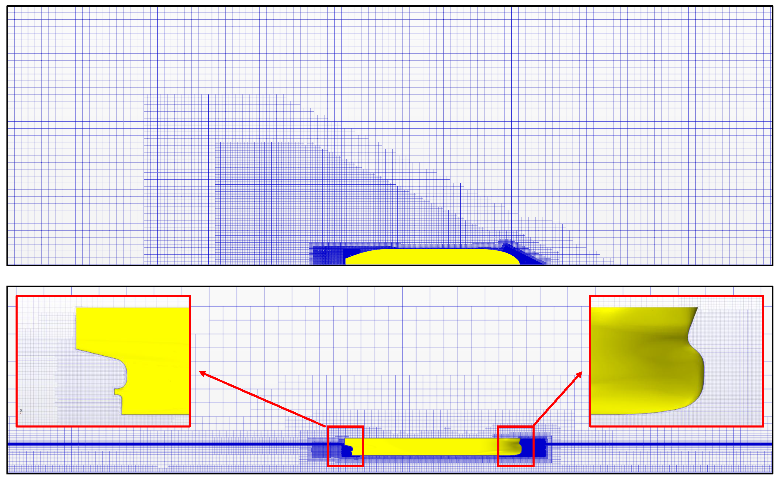
2.3.3. Mesh Generation

The mesh was generated using the automated tools available in Star-CCM+, with the trimmed cell mesher employed to create a predominantly hexahedral cell structure. This technique efficiently produces high-quality grids well-suited for capturing complex fluid interactions. The generation of near-wall cells was facilitated by the prism layer mesher, ensuring the formation of orthogonal cells adjacent to the hull surface. This configuration is known to provide accurate resolution of the boundary layer, which is critical for simulating near-wall flow behavior (mesh for water depth of $150\%ukc$ is illustrated in Figure 8). In scenarios involving shallow water, the bottom boundary is treated as a ’wall’. To ensure consistent wall treatment throughout the simulation, additional prism layers were applied to the bottom of the domain. Local volumetric refinements were introduced around the hull to accurately capture detailed flow phenomena in its vicinity. These refinements ensure a high-resolution representation of intricate flow patterns, especially in regions with rapid changes in flow properties. Furthermore, the mesh was refined in areas where the free surface is expected to deform due to wave interactions and hull motion. This refinement enhances the simulation’s capacity to accurately capture free surface dynamics.

The dimensionless wall distance, $y^{+}$, is a critical non-dimensional parameter in CFD used to assess the adequacy of the near-wall mesh resolution. The value of $y^{+}$ determines the resolution of near-wall flow behavior [38]:

• $y^{+}<5$: Viscous sublayer, dominated by laminar effects, where no wall functions are needed.
• $5<y^{+}<30$: Buffer layer, a transitional zone where turbulence gradually increases.
• $y^{+}>30$: Logarithmic layer, where wall functions are typically employed to model turbulence.

According to ITTC [37], a $y^{+}$ value below 1 is recommended for simulations employing a near-wall turbulence model, whereas a range of $30<y^{+}<500$ is advised when using wall functions. For the model scale, $y^{+}<1$ was achieved, as illustrated in Figure 9, and simulations were conducted under these conditions.

However, these guidelines cover only a limited range of $y^{+}$ values. Moreover, in numerical simulations, $y^{+}$ is not uniform along the length of a ship hull, making near-wall meshing highly complex when adhering strictly to these recommendations. Additionally, for $y^{+}<1$ at high Reynolds numbers ($Re$), the first layer of cells becomes extremely thin, leading to a high aspect ratio that can affect both the stability and accuracy of numerical simulations. In the scale effects study, enforcing the $y^{+}<1$ criterion for full-scale simulations resulted in an extremely high number of cells with large aspect ratios. Since selecting an appropriate $y^{+}$ range is crucial for accurately capturing flow physics while balancing numerical accuracy and computational efficiency, the target $y^{+}$ was set to approximately 60, as shown in Figure 10. All simulations were performed at this setting.

Figure 11 presents the final mesh configurations for the model scale hull at various water depths.

2.3.4. Physics Setup

In this study, all CFD computations were executed using the commercially available RANS solver, Siemens’ Star-CCM+ (version 16.02.008). The finite volume method (FVM) was employed to discretize the integral form of the RANS equations, thereby ensuring the robustness and stability of the numerical framework. A predictor–corrector scheme was implemented to guarantee consistency and convergence across iterative solutions. The volume of fluid (VOF) method was employed to model the free surface and water movement, using the flat wave concept to accurately capture the water-air interface. VOF Method is often the preferred choice due to its excellent mass conservation, ability to handle complex topological changes (e.g., breaking waves and merging interfaces), and computational efficiency. While other methods like level set or smoothed particle hydrodynamics (SPH) may offer higher accuracy in specific cases, they often come with higher computational costs or implementation complexity. VOF strikes a balance between accuracy and efficiency, making it widely used in both academic research and industrial applications.

Table 5. Comparison of free-surface modeling methods in CFD.

Method	Mass Conservation	Topological Changes	Computational Cost	References
VOF	Excellent	Excellent	Low to Moderate	[39]
Level Set	Moderate	Excellent	High	[40]
SPH	Moderate	Excellent	High	[41]
Front Tracking	Good	Moderate	High	[42]
Phase Field	Moderate	Excellent	High	[43]

provides a comparison of different methods for capturing free surfaces.

The realizable $k\text{-}\epsilon$ model is chosen for its balance between computational efficiency and accuracy in ship hydrodynamics. Compared to more advanced models, it reduces computational time by up to 25% while achieving greater accuracy than the $k\text{-}\omega$ model when the viscous sublayer is well resolved [44,45]. It effectively predicts resistance, wake characteristics, and wave-making effects, making it a widely used method for full-scale ship simulations [46,47,48]. This model has proven reliable for confined waterway simulations, accurately capturing ship resistance and hydrodynamic forces [49,50]. Its ability to resolve flow separation and recirculation enhances the prediction of maneuvering forces and resistance in curved channels [51]. Studies also demonstrate its efficiency in simulating frictional and pressure resistance components in submerged bodies and hull forms [25,52]. The two-layer approach further refines near-wall treatment, providing precise resolution of the viscous sublayer while reducing computational costs relative to low-Re turbulence models [53]. Given these advantages, the realizable $k\text{-}\epsilon$ model with a two-layer approach has been adopted for this study.

Additionally, an uncoupled approach was adopted, solving the equations of state independently through a segregated flow model, which balances computational efficiency and solution accuracy. The spatial discretization employed second-order upwind schemes for convective fluxes and second-order central schemes for diffusion terms, enhancing the solution’s accuracy. The SIMPLE (Semi-Implicit Method for Pressure-Linked Equations) algorithm was implemented to ensure solution convergence. To reduce simulation complexity and computational cost, the ship model was fixed in both heave and pitch DOFs.

2.4. Verification and Validation Study —V&V

Verification and validation are critical processes in the context of CFD simulations as they ensure the accuracy and reliability of numerical results. Verification serves to confirm the correctness of numerical methods. Validation, on the other hand, involves a comparison of simulation results with experimental data to assess their physical accuracy. These processes are vital for establishing credibility and minimizing errors in CFD simulations.

2.4.1. Verification Study

The term numerical uncertainty refers to the discrepancy between a numerical result obtained through computational methods and its exact analytical solution. Various types of numerical errors contribute to this uncertainty [54], as detailed below:

• Round-off errors: These errors arise from the finite precision of numerical representations within a computer. While typically minor, they can accumulate during computations, especially as grid refinement increases, potentially impacting the results in certain scenarios. In this study, double-precision calculations were employed to mitigate round-off errors, rendering them negligible in most practical cases.
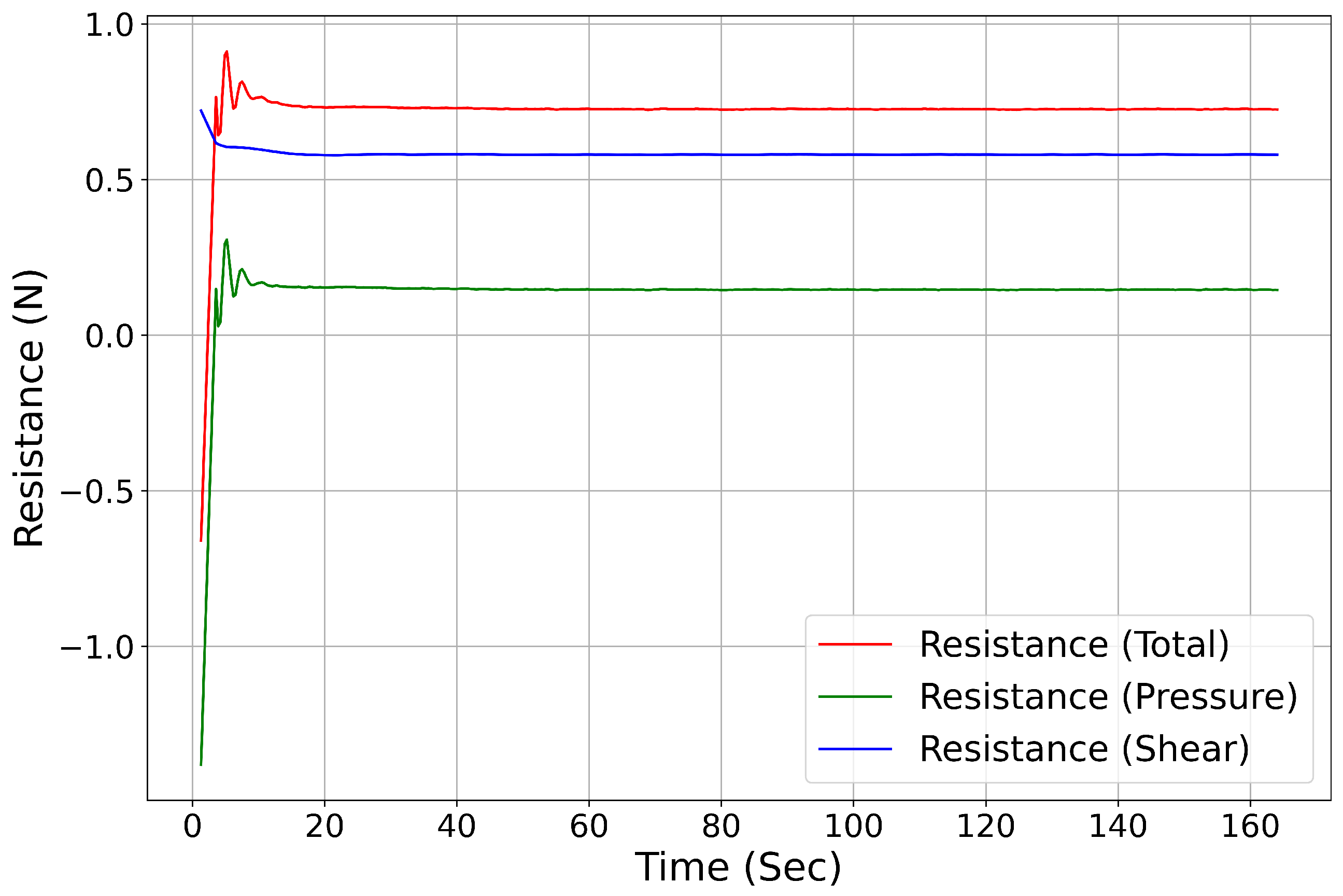
• Convergence errors: Convergence errors occur when iterative methods, often used to solve discretized mathematical models, fail to achieve full convergence. This is particularly relevant when dealing with nonlinear equations or for computational efficiency. To address convergence errors, double-precision schemes were used, and an adequate number of iterations were ensured. Total and frictional resistance values were closely monitored, confirming that convergence errors were negligible once these parameters stabilized or exhibited periodic behavior, indicating sufficient convergence of the solution, as shown in Figure 12.
• Programming errors: Programming errors can introduce unpredictable results if not identified and addressed. However, in this study, no specific analysis of programming errors was performed, as the simulation software used has already undergone rigorous verification and validation, ensuring its accuracy and reliability.
• Discretization errors and representation errors: Considering the above, the verification process primarily focused on discretization errors, covered in Section 2.4.2, which typically constitute the largest component of numerical error in CFD simulations. These errors stem from the approximation of continuous equations into discrete forms, introducing numerical inaccuracies.

Through the systematic evaluation and mitigation of these error sources, the verification process ensures that the numerical framework is robust and reliable, providing a strong foundation for subsequent validation efforts.

2.4.2. Discretization Error Analysis

This section focuses on the analysis of discretization errors, which are critical to ensuring the accuracy of CFD simulations. The following areas were investigated:

• Spatial Convergence Study: The impact of grid resolution on numerical accuracy was evaluated through systematic mesh refinement, commonly known as a grid/mesh sensitivity study, with convergence rates quantified using methods such as Richardson extrapolation.
• Temporal Convergence Study: The influence of time step size on simulation accuracy was analyzed to ensure temporal resolution independence, balancing numerical precision and computational efficiency.

The Grid Convergence Index (GCI) method [55] was employed for the verification study to determine appropriate grid spacing and timestep sizes. This method is based on Richardson extrapolation [56]. Verification studies were conducted under shallow water conditions (150% ukc) at model scale ($\lambda =75$). This study focused on barehull resistance with the free surface present at a corresponding speed of 11 knots (full-scale speed). The optimal grid spacing identified from the grid refinement study under shallow water conditions (150% ukc) was then applied to other water depths, with only the water depth being adjusted to the desired condition. The CFD simulation verification method is explained in the following paragraphs. For each study, three different grid resolutions were employed, designated as fine, medium, and coarse meshes, corresponding to cell counts $N_1$, $N_2$, and $N_3$, respectively. During the spatial convergence study, the near-wall characteristics of the prism layer mesh surrounding the hull and the bottom of the domain, specifically designed for shallow water conditions, were held constant while systematically varying the grid density. Refinement ratios, $r_{21}$ and $r_{32}$, are calculated as follows.

$$r_{{21}_{Grid}}=\sqrt[3]{{\displaystyle \frac{N_1}{N_2}}}$$

(3)

$$r_{{32}_{Grid}}=\sqrt[3]{{\displaystyle \frac{N_2}{N_3}}}$$

(4)

For the timestep, refinement ratios are calculated as follows:

$$r_{{21}_{TimeStep}}={\displaystyle \frac{T_1}{T_2}}$$

(5)

$$r_{{32}_{TimeStep}}={\displaystyle \frac{T_2}{T_3}}$$

(6)

The difference between the scalar solutions ($\epsilon$) is calculated using the following equations:

$${\epsilon }_{32}={\varphi }_3-{\varphi }_2$$

(7)

$${\epsilon }_{21}={\varphi }_2-{\varphi }_1$$

(8)

Here, ${\varphi }_k$ represents the key variables (where k = 1, 2, 3 for fine, medium and coarse meshes). In this study, total resistance was selected as the key variable or scalar quantity.

The convergence ratio (R) is defined as follows:

$$R={\displaystyle \frac{{\epsilon }_{21}}{{\epsilon }_{32}}}$$

(9)

The convergence or divergence of a solution can be classified into four distinct conditions [57], summarized as follows:

$$\begin{array}{cccc}& 0<R<1\hfill & & (\text{Monotonic}\text{convergence})\hfill \\ & R<0,\left|R\right|<1\hfill & & (\text{Oscillatory}\text{convergence})\hfill \\ & R>1\hfill & & (\text{Monotonic}\text{divergence})\hfill \\ & R<0,\left|R\right|>1\hfill & & (\text{Oscillatory}\text{divergence}).\hfill \end{array}$$

The approximate relative error, $e_a^{21}$, is calculated using the following equation:

$$e_a^{21}=\left|{\displaystyle \frac{{\varphi }_1-{\varphi }_2}{{\varphi }_1}}\right|$$

(10)

The observed order of accuracy, $p_a$, is determined by the following:

$$p_a={\displaystyle \frac{1}{ln\left(r_{21}\right)}}\left|ln\left|{\displaystyle \frac{{\epsilon }_{32}}{{\epsilon }_{21}}}\right|+q\left(p_a\right)\right|$$

(11)

Here, $q\left(p_a\right)$ and s are defined as follows:

$$q\left(p_a\right)=ln\left({\displaystyle \frac{r_{21}^{p_a}-s}{r_{32}^{p_a}-s}}\right)$$

(12)

$$s=\mathrm{sign}\left({\displaystyle \frac{{\epsilon }_{32}}{{\epsilon }_{21}}}\right)$$

(13)

The values of $p_a$ and $q\left(p_a\right)$ are determined through a numerical solution process. The uncertainty level of the numerical solution for the fine grid is then calculated using the following equation:

$$GC{I}_{fine}^{21}={\displaystyle \frac{F_s{e}_a^{21}}{r_{21}^p-1}}$$

(14)

Here, $F_s$ is a safety factor. When $0.5\le p_a\le 2.1$, $F_s=1.25$; otherwise, $F_s=3$.

For the spatial convergence study, $N_2$ and $N_3$ were generated by systematically coarsening $N_1$ in the x, y, and z directions. Following the recommended guidelines [58], the refinement ratio between the meshes under consideration was maintained at greater than 1.3. The key parameters used to calculate the spatial discretization error are provided in

Table 6. Spatial and temporal discretization errors for Aframax CFD simulations.

Parameters	Mesh	Time-Step
$N_1$	2.840 M	0.0239 s
$N_2$	0.752 M	0.0338 s
$N_3$	0.203 M	0.0478 s
$r_{21}$	1.56	1.41
$r_{32}$	1.55	1.41
${\varphi }_1$	2.76143	2.76143
${\varphi }_2$	2.72728	2.76242
${\varphi }_3$	3.6217	2.76858
${\epsilon }_{32}$	0.894	0.00616
${\epsilon }_{21}$	−0.034	0.00099
R	−0.038	0.16
	Oscillatory convergence	Monotonic convergence
s	−1	1
$e_a^{21}$ (%)	0.012	0.036
q	0.04	0
p	7.47	5.283
$GC{I}_{fine}^{21}$ (%)	0.059	0.009

. The results indicate that the numerical uncertainty associated with spatial discretization remains within acceptable limits. Therefore, the fine grid ($N_1$) was selected for the analysis of scale effects, ensuring reliable and accurate results.

For the temporal convergence study, the selection of an appropriate time step ($\Delta t$) is critical in CFD simulations to ensure accuracy and stability. The Courant–Friedrichs–Lewy (CFL) number is widely used to evaluate the convergence of simulated flows. This principle assumes that for fluid flow over a discrete spatial grid, an appropriate combination of time step and grid spacing is required to resolve fluid properties such as velocity and pressure at each grid point. To meet this requirement, the condition $CFL\le 1$ must be satisfied. The recommended time step [37] is given by the following:

$$\Delta t=0.005\sim 0.01{\displaystyle \frac{L}{U}}$$

(15)

In this study, the smallest recommended time step is used to simulate barehull simulations with the free surface:

$$\Delta t=0.005{\displaystyle \frac{L}{U}}$$

(16)

As shown in the Table 6, the numerical uncertainties associated with this chosen time step are minimal. Thus, the smallest time step is used for all subsequent analyses, ensuring a high degree of accuracy and reliability in the results.

2.4.3. Validation Study

After the verification of the numerical setup, additional validation against existing data, such as experimental results, is essential to enhance its reliability. However, as discussed in Section 1, experimental data for shallow water conditions are extremely scarce. Specifically, no documented experimental measurements of the wake field in (very) shallow water were found by the author. Moreover, during the model scale experiments of the Aframax hull form conducted for this research, flow visualization at the aft of the ship was not performed. Given these limitations, the following approach was adopted for the validation study:

• Validation using experimental results for the Aframax model ship in shallow water, with total resistance as the reference parameter.
• Validation against EFD/CFD results from the literature for the KVLCC2 hull form (both model and full scale) in deep water, using total resistance as the reference parameter.
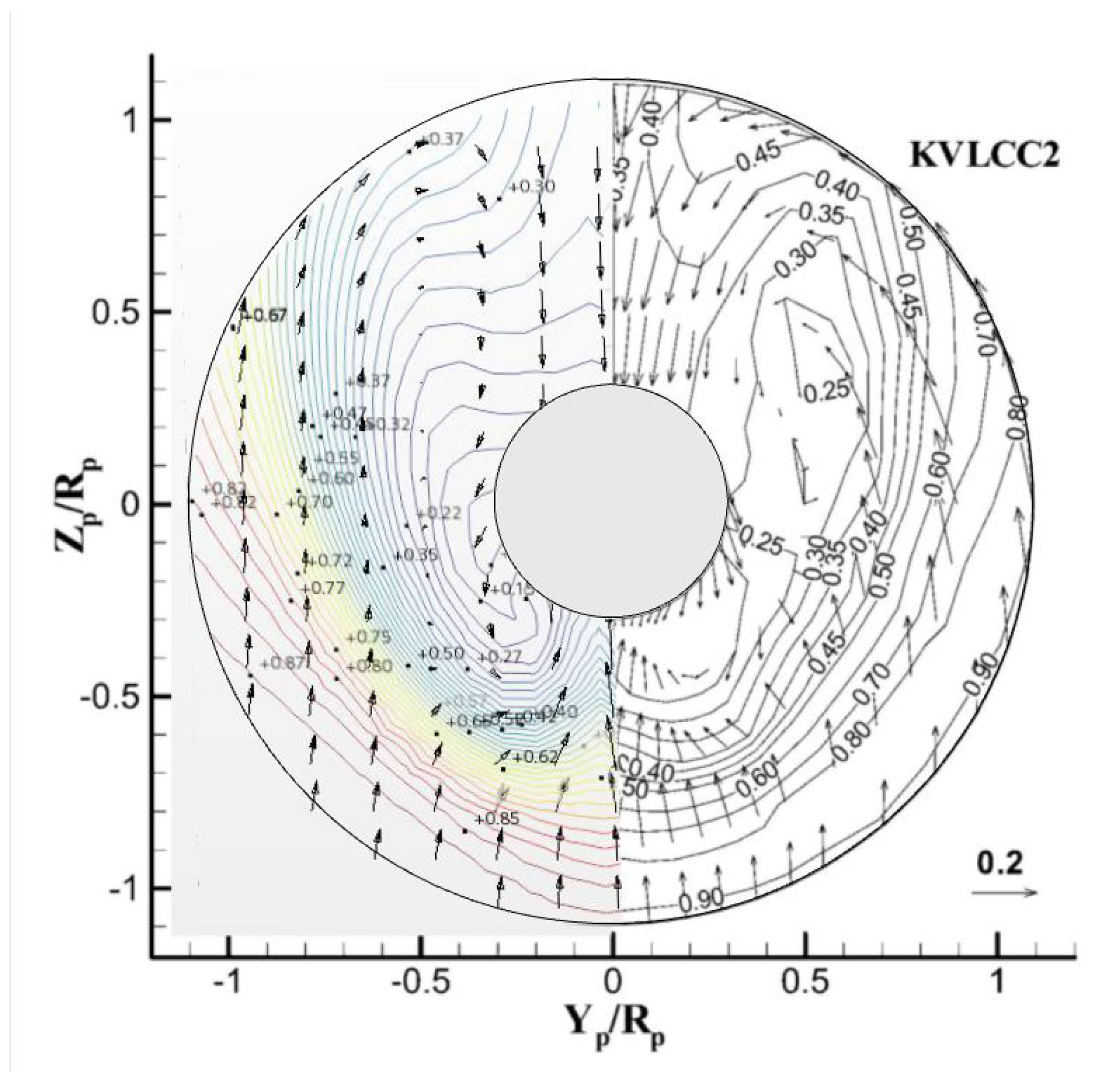
• Validation of the wake field distribution against experimental results for the KVLCC2 model ship in deep water.

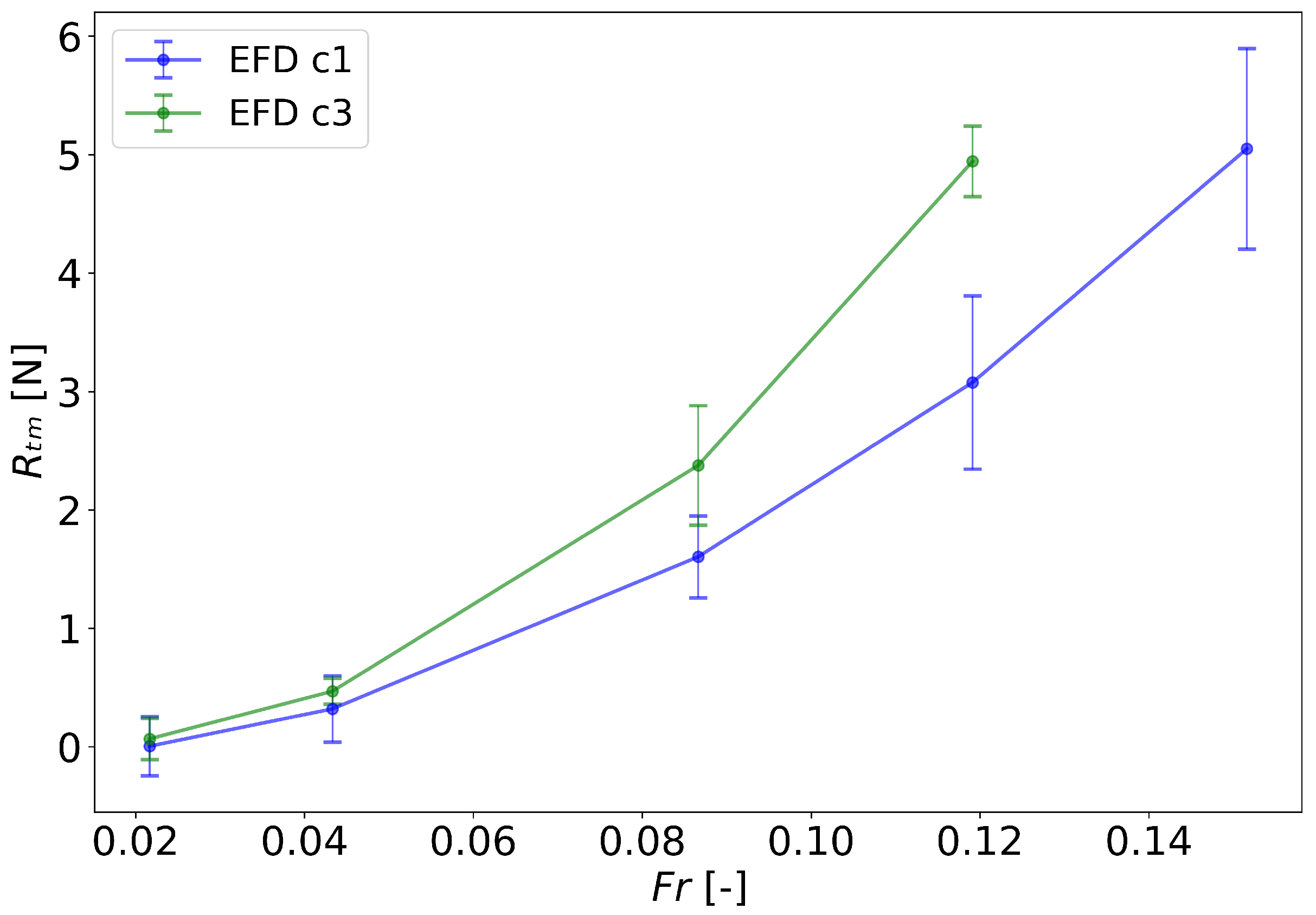
2.4.4. Validation with Aframax Hull Form—Shallow Water

As the first step, the Aframax model ship was used as the reference, and the total resistance in two shallow water conditions obtained from numerical simulations was compared to experimental results. These comparisons are illustrated in Figure 13 and summarized in

Table 7. Comparison of EFD and CFD results for Aframax model ship’s total resistance at various speeds and water depths.

	EFD ${\mathit{R}}_{\mathit{t}}$(N)		CFD ${\mathit{R}}_{\mathit{t}}$(N)		% Difference
Fr [-]	${\mathit{c}}_{\mathbf{1}}$	${\mathit{c}}_{\mathbf{3}}$	${\mathit{c}}_{\mathbf{1}}$	${\mathit{c}}_{\mathbf{3}}$	${\mathit{c}}_{\mathbf{1}}$	${\mathit{c}}_{\mathbf{3}}$
0.0217	0.0056	0.0672	0.0060	0.0700	7.78	4.12
0.0433	0.3206	0.4693	0.4023	0.4125	25.50	−12.11
0.0866	1.6048	2.3764	1.5504	2.0492	−3.39	−13.77
0.1191	3.0771	4.9436	2.8672	4.3274	−6.82	−12.46
0.1516	5.0503		4.5700		−9.51

, covering a range of speeds.

The water conditions $c_1$ and $c_3$ correspond to $150\%ukc$ and $20\%ukc$ water depth conditions, respectively. A relatively good agreement is observed between the EFD and CFD results. While the CFD values are well within the experimental uncertainty limits, the numerical setup tends to under-predict total resistance, particularly when considering average values. At a medium speed of $Fr=0.087$, equivalent to 8 knots at full scale, the percentage differences between the EFD and CFD results are −3.4% and −13.8% for $150\%ukc$ and $20\%ukc$, respectively. At higher speeds, the percentage differences increase to −9.51 percent and −12.46 percent for $150\%ukc$ and $20\%ukc$, respectively. Differences observed between CFD and the experimental fluid dynamics (EFD) results can be attributed to discrepancies in modeling and experimental setups. In the EFD experiments, the ship was allowed to heave and pitch freely, accommodating the natural movements that occur in real-world scenarios. This freedom can lead to variations in the wetted surface area of the hull, which in turn affects resistance measurements. Conversely, in the CFD simulations, the ship’s heave and pitch degrees of freedom were fixed. This simplification makes the computational process more economical but can lead to discrepancies, especially at higher speeds where dynamic effects are more pronounced. However, in shallow water conditions, vessels generally maintain low to medium speeds to minimize the risk of grounding. When navigating through canals, legal speed restrictions are often enforced. For instance, the Suez Canal Authority imposes a maximum speed limit of 7 knots [59], while in the Panama Canal, vessel speeds are regulated between 6 and 10 knots depending on the canal segment and the type of ship [60]. Despite these differences, the general agreement between CFD and EFD data at medium speeds, which are typical in confined waters, validates the applicability of the current study for practical engineering purposes. This approach balances computational efficiency with sufficient accuracy. Notwithstanding these discrepancies, it is presumed that this variation will not markedly influence the wake fraction, given that the wake fraction tends to remain relatively consistent across varying speeds. Consequently, these discrepancies should not impact the outcomes of subsequent studies.

2.4.5. Validation with KVLCC2 Hull Form—Deep Water and Full Scale

To validate the numerical setup for deep water and full-scale simulations, the KVLCC2 hull form was used as a reference. The total resistance coefficients and nominal wake fraction obtained from the CFD simulations at the design speed (15.5 knots at full scale) were compared with values reported in the literature. These comparisons, which detail the total resistance coefficient and nominal wake fraction for the KVLCC2 model ($\lambda$ = 58), are presented in

Table 8. Comparison of total resistance coefficient for KVLCC2 in model ($\lambda$ = 58) and full scale at $Fr$ = 0.142 from CFD and literature sources.

Scale	${\mathit{C}}_{\mathit{t}}$ × 10−3	${\mathit{C}}_{\mathit{t}}$ × 10−3 (Literature)	Source	%Diff
Model Scale	4.100	4.110	EFD [61]	−0.24
		4.176	CFD [62]	−1.82
		4.176	CFD [63]	−1.82
Full Scale	1.907	1.722	CFD [64]	+6.26
		1.806	CFD [62]	+5.61
		1.810	CFD [63]	+5.38

and

Table 9. Comparison of wake fraction for KVLCC2 in model ($\lambda$ = 58) and full scale at $Fr$ = 0.142 from CFD and literature sources.

Scale	${\mathit{w}}_{\mathit{CFD}}$	${\mathit{w}}_{\mathit{literature}}$	Source	%Diff
Model Scale	0.524	0.487	Corrected EFD [61]	+7.57
		0.550	CFD [62]	−4.70
Full Scale	0.310	0.336	Corrected EFD [61]	−7.71
		0.320	CFD [62]	−3.24

, respectively. The actual CFD results were used as the basis for calculating the relative differences. For the model scale simulations, the total resistance coefficient for the KVLCC2 hull form agreed well with the experimental and CFD data available in the literature, with relative differences remaining below 2%. In the full-scale simulations, the current results for the KVLCC2 hull form showed a good agreement with other full-scale CFD results reported in the literature, with relative differences below 6%.

For the wake fraction, the present simulation exhibited a deviation of less than 8% compared to both experimental data and CFD results at the model scale. Furthermore, the simulation results demonstrated strong agreement with full-scale CFD predictions reported in the literature, with discrepancies remaining below 8%. This consistency highlights the reliability of the numerical approach in capturing the wake characteristics across different scales.

The wake field distribution ($v_a/v$) on the propeller disk from the current CFD study was evaluated against experimental data [61], as shown in Figure 14. The CFD setup successfully reproduces the characteristic hook shape observed in the wake field, albeit with slightly reduced intensity. Nevertheless, the overall wake field shows good agreement with the experimental data. These results suggest that the chosen mesh and numerical setup are robust and reliable, providing a strong foundation for further analysis with confidence.

3. Results and Discussion

The wake field is the flow resulting from the relative motion between a hull and the surrounding fluid. It includes the velocity disturbances and vortices produced by the hull during its movement in water. The nominal wake field is the wake at the propeller disc in the absence of propeller action and is considered an important parameter in propeller design and performance prediction. It comprises three components [65]: potential wake ($w_p$), frictional wake ($w_f$) and wave wake ($w_w$). These components are combined in Equation (17):

$$w=w_p+w_f+w_w$$

(17)

The potential wake arises in an ideal fluid with no viscosity, where flow is influenced solely by the hull’s shape. The frictional wake results from the viscous nature of water, creating a velocity gradient near the hull surface. The wave wake is caused by gravity waves generated due to the hull’s motion. Together, these components define the overall wake field and its impact on propulsion efficiency and cavitation characteristics.

The nominal wake fraction ($w_n$) quantifies the average reduction in axial velocity within the wake in comparison to the undisturbed freestream velocity. This reduction is measured across the propeller disc area. The derivation of this parameter involves integrating surface values using Equation (18), which involves computing velocities at various radial and angular positions within the wake.

$$w_n={\displaystyle \frac{\underset{r_B}{\overset{R}{\int }}{w}^{\prime }\left(r\right)·2\pi rdr}{\underset{r_B}{\overset{R}{\int }}2\pi rdr}}={\displaystyle \frac{2}{R^2-r_B^2}}\underset{r_B}{\overset{R}{\int }}{w}^{\prime }\left(r\right)·rdr$$

(18)

where $w^{\prime }\left(r\right)$ is the circumferential mean wake fraction at a given radius r. The term $r_B$ refers to the radius of the propeller boss, whereas R indicates the radius of the propeller itself. In the following sections, the results are presented for the effects of water depth and scale on the wake field and nominal wake fraction in shallow water.

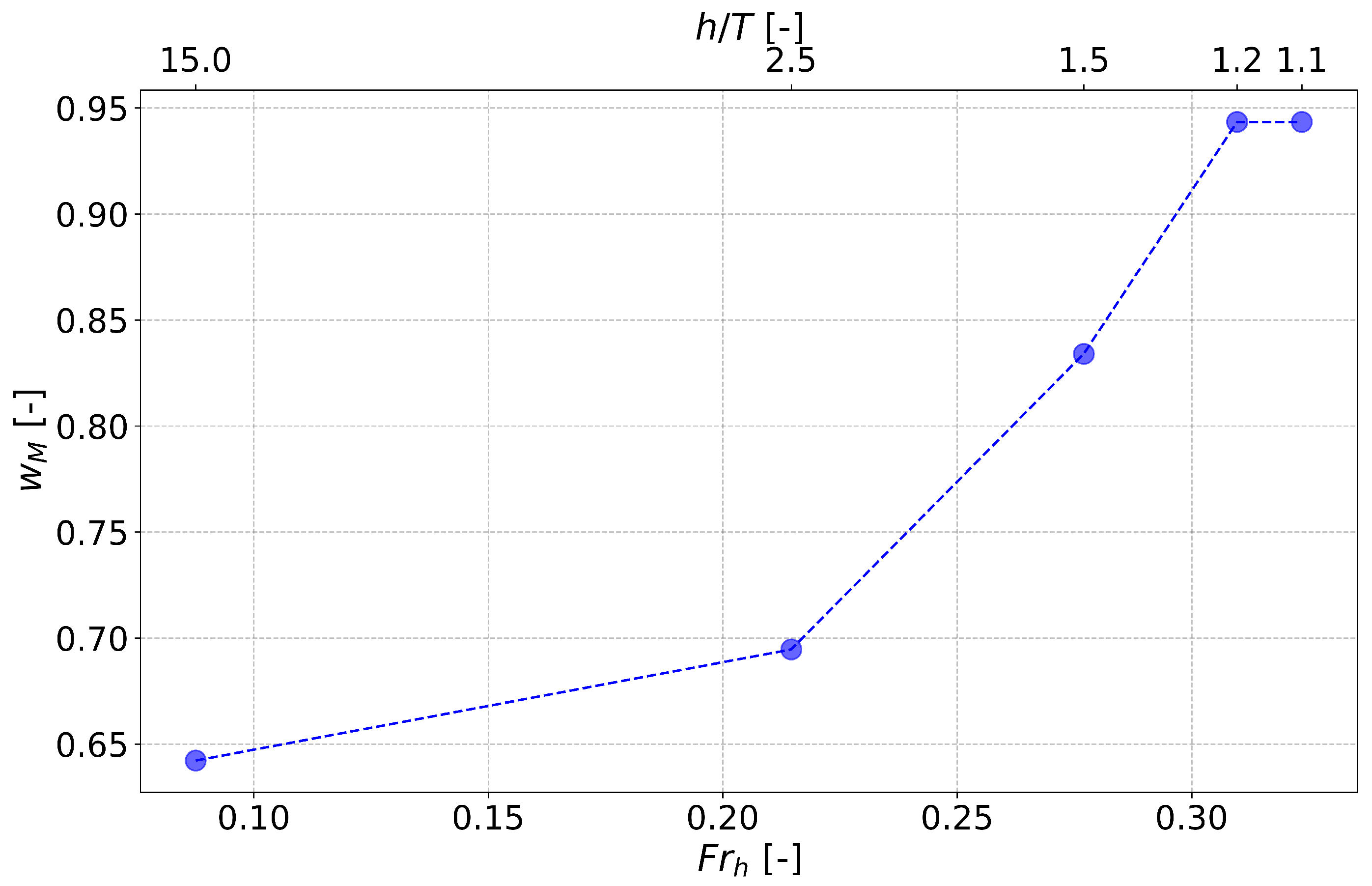
3.1. Water Depth Effect on Nominal Wake Fraction

A comprehensive analysis was conducted to investigate the impact of water depth on the nominal wake fraction for the Aframax hull form at model scale, as illustrated in Figure 15. The x-axis of the figure represents five different water depths, which are further detailed in Table 3. This configuration facilitates a clear and effective comparative assessment. A notable increase in the nominal wake fraction is evident as water depth decreases. This observation underscores the sensitivity of the nominal wake fraction to changes in water depth, particularly in confined environments. The data reveal a significant disparity in nominal wake fractions between the deepest and very shallow water conditions ($h/T=1.1$), with a relative difference of approximately 32% for the model scale. As water depth decreases, the vessel experiences an increase in viscous resistance, primarily due to the reduced clearance between the vessel’s hull and the seabed or riverbed, which limits the flow area. This spatial constraint impacts not only the displacement flow around the hull but also the overall flow dynamics at the ship’s stern. This results in a greater velocity deficit at the propeller plane, which negatively impacts the ship’s efficiency and operational performance. This intricate interplay between water depth and ship hydrodynamics underscores the necessity for a comprehensive consideration of these effects in naval architecture and marine operations.

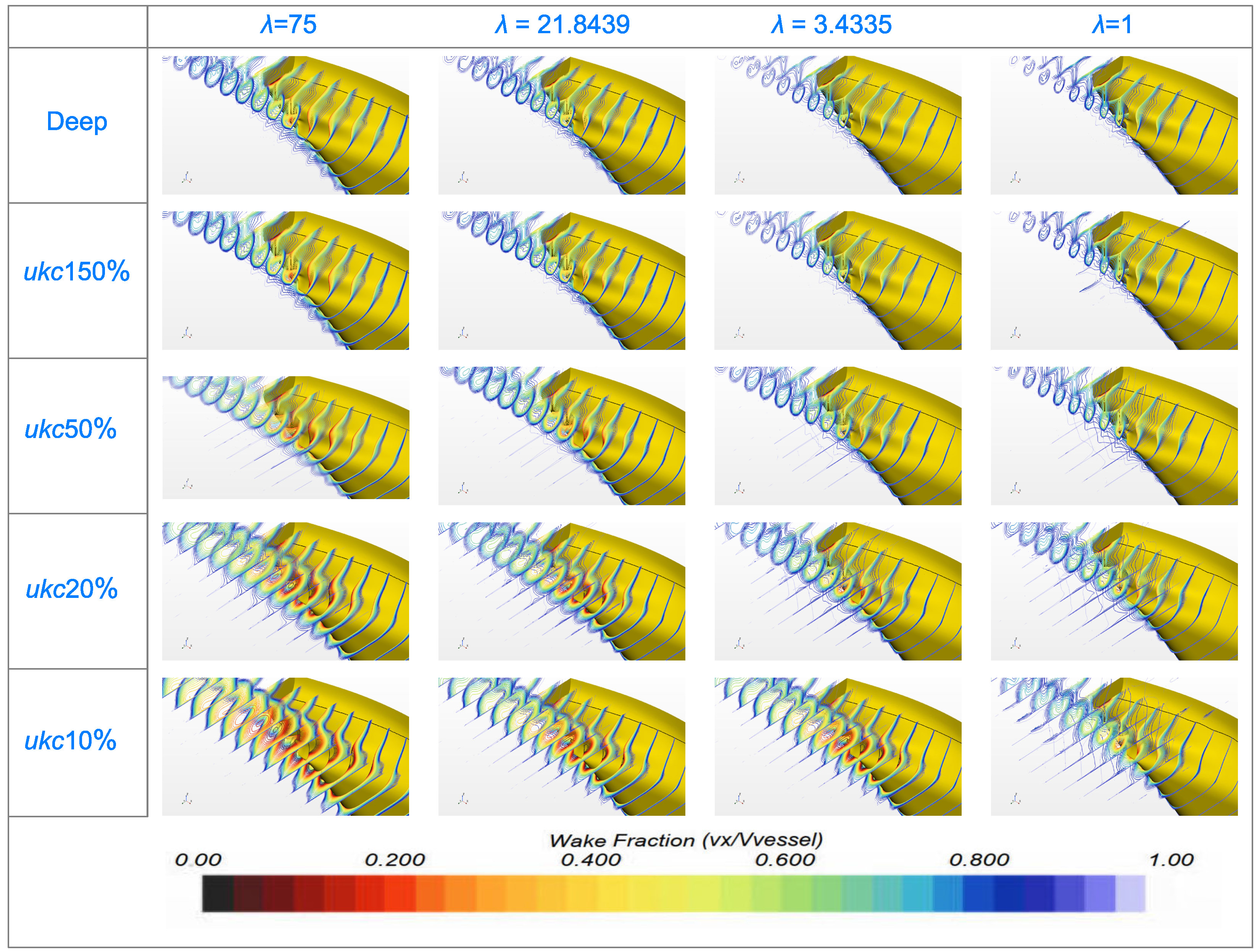
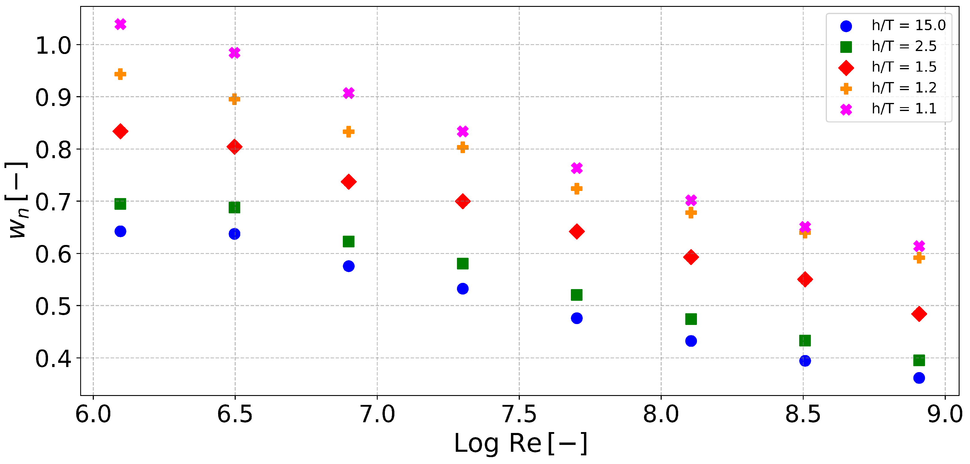
3.2. Scale Effect on Nominal Wake Fraction in Shallow Water

To explore the scale effects on the wake field and nominal wake fraction, numerical simulations were conducted at a Froude number of $Fr=0.087$. This corresponds to 8 knots for the full-scale ship, and the simulations were performed across multiple ship scales and water depths. Detailed information regarding these simulations can be found in Table 2. Comprehensive analyses were carried out in both deep and shallow water conditions, enabling a thorough investigation into how water depth variations influence the hydrodynamic behavior of ships at different scales.

The nondimensional axial velocity contours at the aft plane of the Aframax hull form are presented in Figure 16 at various scales and for different water depths. For the sake of clarity, the figure selectively displays only four of the eight scales that were analyzed, with the intention of highlighting the key trends with greater distinction. The figure illustrates that as the Reynolds number increases, the thickness of the boundary layer decreases, becoming notably thinner for the full-scale model compared to the model scale. Additionally, the axial velocity contours become more concentrated and align closer to the ship’s center plane. The stern of the model scale ship exhibits a larger high-wake area compared to the full-scale ship, which has a significantly smaller high-wake area. This disparity suggests that the flow velocity at the model scale ship’s stern is lower than that at the full-scale ship’s stern. Furthermore, an increase in the velocity deficit with decreasing water depth is evident. Furthermore, in shallow water conditions, specifically when the ratio $h/T$ is less than or equal to 1.2, the interaction between the vessel’s hull boundary layers and the bottom surface becomes more pronounced, with the effects of shallow water becoming increasingly significant as the Reynolds number increases.

As illustrated in Figure 17, the complete wake field surrounding the stern of the ship captures the development of the boundary layer along the ship’s hull. This visualization distinctly demonstrates the boundary layer thickening as it progresses toward the aft end of the hull. It is noteworthy that the relative thickness of the boundary layer exhibits a decrease in proportion with an increase in the Reynolds number. As the flow transitions from the bow towards the stern, the growth of the boundary layer can be attributed to the increased frictional resistance and viscous effects along the hull’s surface. This thickening is more pronounced at lower Reynolds numbers, where viscous forces predominate over inertial forces. Conversely, at higher Reynolds numbers, prevalent in full-scale ships or at higher velocities, the boundary layer becomes thinner and more streamlined, signifying a scale-dependent interaction between the fluid flow and the ship’s surface. The proximity of the seabed has been shown to significantly influence the vessel’s boundary layer, causing it to thicken earlier in the flow process. In particularly shallow water, when the ratio of the depth to the temperature, $h/T$, is less than or equal to 1.2, there is a noticeable enlargement of the boundary layer due to the convergence of boundary layers from the ship’s hull and the bottom surface.

Figure 18 displays the contours of mean axial velocity at the propeller plane, expressed as the nominal wake fraction. As observed in earlier figures, the wake field at the propeller plane exhibits substantial dependencies on scale and water depth. A distinguishing characteristic of the smaller model scales is the presence of a “hook-like” region within the wake contours. This hook-like formation at the propeller plane is a characteristic of low-speed full ships, largely due to the development and movement of bilge vortices. Conversely, for full-scale vessels, the wake tends to be more concentrated along the centerline, indicative of a more streamlined flow compared to smaller scales. Furthermore, a decrease in water depth leads to a marked reduction in flow at the propeller plane, resulting in higher nominal wake fraction values. This observation underscores the substantial influence of shallow water conditions on ship hydrodynamics. This effect is particularly pronounced for model scale ships compared to full-scale ships, underscoring the scale-sensitive nature of hydrodynamic behaviors and emphasizing the importance of considering these effects in design and simulation studies. This figure underscores the significant influence of shallow water conditions, emphasizing their crucial role for ships operating in such environments.

The values of the nominal wake fraction derived from CFD simulations across all case studies are depicted in Figure 19. The abscissa of this figure plots the Reynolds number ($Re$) on a logarithmic scale, and the y-axis represents the nominal wake fraction at various water depths. A clear pattern emerges, underscoring the variation of the nominal wake fraction with both Reynolds number and water depth. It is evident that water depth exerts a substantial influence on the relationship between $Re$ and the nominal wake fraction. As the Reynolds number increases, the mean axial wake fraction decreases, thereby establishing a non-linear relationship between these variables. Additionally, the impact of water depth is evident, with nominal wake fractions increasing as water depths decrease. The variation in wake fractions between deep and medium-deep waters is minimal; however, there is a notable increase in wake fractions as water depths reach shallow or very shallow levels. Specifically, in full-scale scenarios, the mean axial wake fraction decreases by 77% in deep water and by 69% in shallow water (with $h/T=1.1$) compared to the model scale ($\lambda =75$). This finding underscores the notion that while the overarching tendency of a decrease in wake fraction with an increase in Reynolds number persists across diverse water depths, the magnitude of this phenomenon is more pronounced in shallow water. This finding underscores the critical importance of incorporating both Reynolds number and water depth when assessing the scale effects on wake fractions.

To simplify the analysis, scenarios involving deep water and shallow water (where $h/T\le 2.5$) are analyzed separately. For deep water, the equation for the nominal wake fraction was developed by fitting data points, as illustrated in Figure 20 and detailed in Equation (19). The curve fit displays a high degree of precision with an $R^2$ value of 0.9875, indicating a robust correlation. The coefficients for this equation are provided in

Table 10. Regression coefficients for the empirical equation predicting nominal wake fraction in deep water.

${\mathit{a}}_{\mathbf{1}}$	${\mathit{a}}_{\mathbf{2}}$	${\mathit{a}}_{\mathbf{3}}$
1.3076	−0.1049	−0.0002

.

$$w_{n\left(deep\right)}=a_1+a_2\left(LogRe\right)+a_3{\left(LogRe\right)}^2$$

(19)

For shallow water, a correlation has been established between the wake fraction, water depth, and Reynolds number using the least squares method. This relationship is illustrated in Figure 21 and expressed in Equation (20), exhibiting a high degree of precision with an $R^2$ value of 0.9913. The coefficients for this equation are detailed in

Table 11. Regression coefficients for the empirical equation predicting nominal wake fraction in shallow water.

${\mathit{b}}_{\mathbf{1}}$	${\mathit{b}}_{\mathbf{2}}$	${\mathit{b}}_{\mathbf{3}}$	${\mathit{b}}_{\mathbf{4}}$	${\mathit{b}}_{\mathbf{5}}$	${\mathit{b}}_{\mathbf{6}}$
2.88604	−0.21110	−0.95672	0.00313	0.02097	0.17098

.

$$w_{n\left(shallow\right)}=b_1+b_2\left(LogRe\right)+b_3\left({\displaystyle \frac{h}{T}}\right)+b_4{\left(LogRe\right)}^2+b_5\left({\displaystyle \frac{h}{T}}\right)\left(LogRe\right)+b_6{\left({\displaystyle \frac{h}{T}}\right)}^2$$

(20)

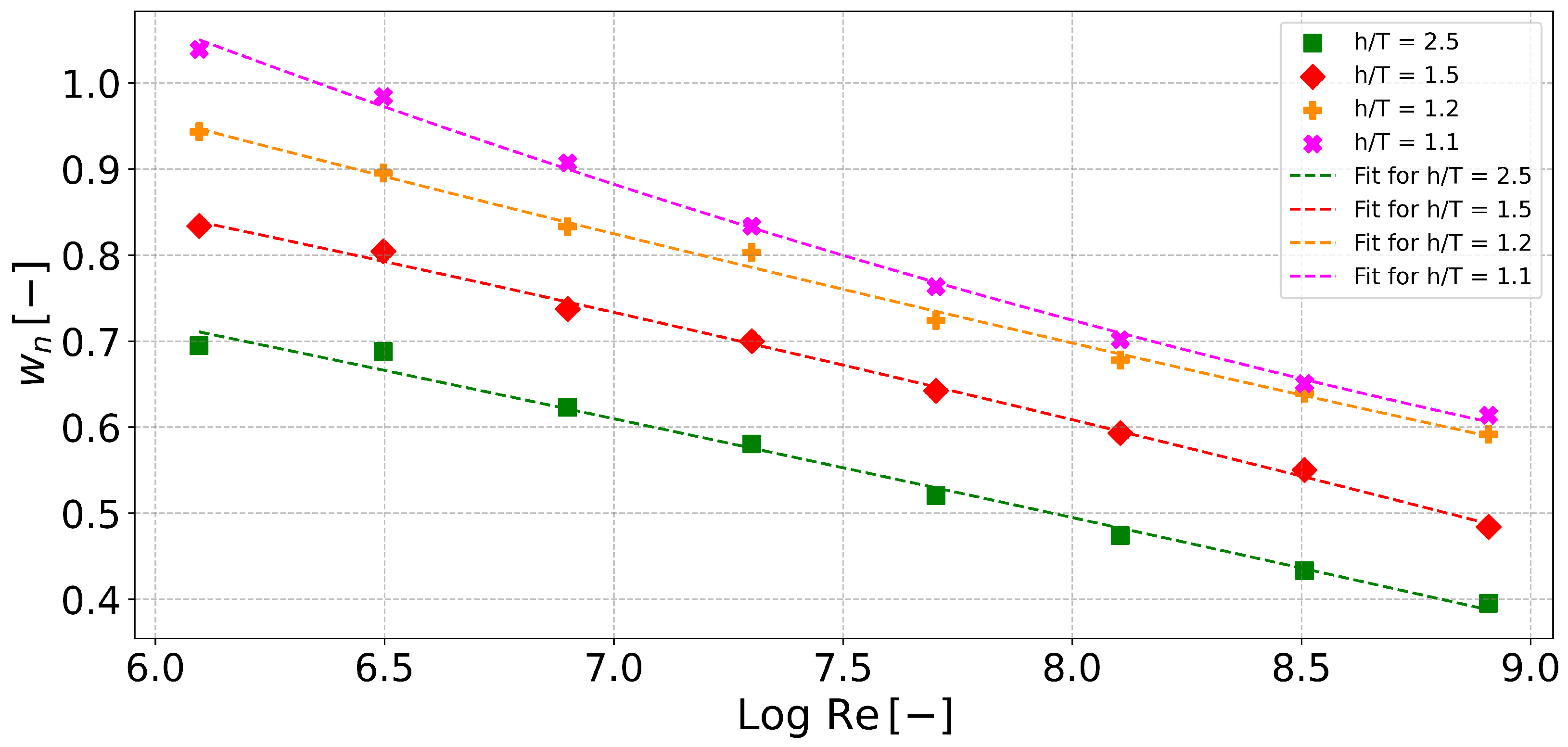
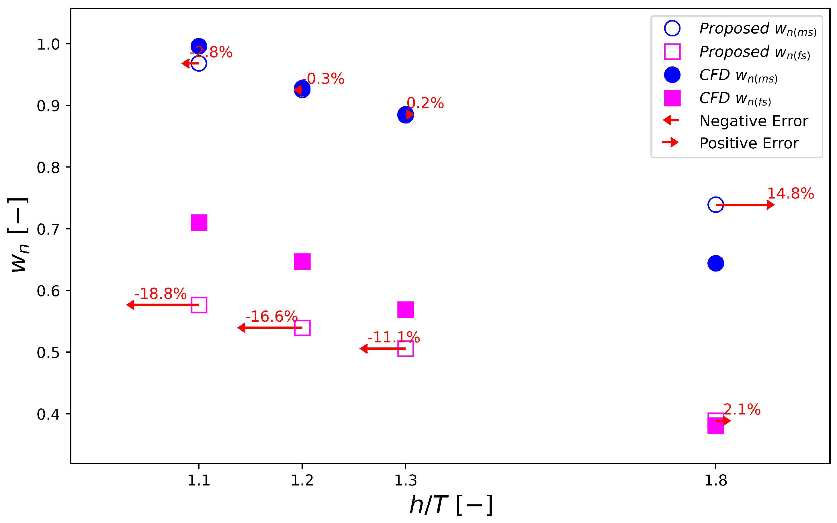
3.3. Application of the Proposed Equation for Nominal Wake in Shallow Water

To evaluate the applicability of the proposed equation (Equation (20)) for calculating the nominal wake fraction in shallow water, the KVLCC2 hull form was chosen as a reference model. This choice aims to verify the applicability of the equation under different conditions using a well-documented and representative hull form. In addition, the KVLCC2 shares similar key dimensional ratios such as $L/B$, $L/T$, and the block coefficient ($C_b$) with the Aframax hull form, as shown in Table 1. However, the aft section of the KVLCC2 has different characteristics, which could potentially affect the wake field.

CFD simulations were performed for the model ($\lambda$ = 75) and full-scale KVLCC2 hull form at four shallow water depths ($h/T=1.1,1.2,1.3$, and $1.8$) and forward speed equivalent to 11 knots at full scale using the same numerical setup as discussed in Section 2. The results of these simulations are then compared with the predictions of the proposed equation for determining the nominal wake fraction in shallow water, as shown in Figure 22. This figure plots the nominal wake fraction against water depth and demonstrates that the nominal wake fraction increases as water depth decreases. It also shows that the nominal wake fraction of the model scale is consistently higher than that of the full scale, emphasizing the dependence on the Reynolds number ($Re$).

The analysis demonstrates that the proposed equation (Equation (20)) exhibits a high degree of accuracy in predicting the nominal wake fraction for the model scale in shallow water, with a discrepancy of less than 3% compared to the CFD results. However, the accuracy of this equation is reduced for full-scale ships in shallow water, with discrepancies reaching up to 19%. The observed trends in shallow water manifest as monotonic while the variations in the nominal wake fraction at medium water depths are more pronounced for the model scale. Given that the proposed equation was derived using data from a single hull form, the Aframax, its applicability to other hull forms may not be universal. Consequently, further research is necessary to develop a more generalized equation that can be reliably applied to different hull forms.

4. Conclusions and Recommendations

This study presents a comprehensive investigation into the scale effects on the wake field and nominal wake fraction in shallow water, employing both experimental model testing and CFD simulations. The main findings reveal that as water depth decreases, the nominal wake fraction increases significantly, leading to greater velocity deficits at the propeller plane. Conversely, as the Reynolds number increases, the nominal wake fraction decreases due to the thinner boundary layers observed in full-scale ships compared to model scale ships.

A key contribution of this work is the identification of a nonlinear relationship between Reynolds number and nominal wake fraction, which was previously underexplored, particularly in shallow water conditions. The developed predictive equation for nominal wake fraction provides an improved tool for estimating wake field characteristics. This equation was further tested against CFD results for the KVLCC2 hull form, confirming its applicability but also highlighting the need for additional refinements to improve its reliability across diverse hull forms. Unlike previous studies that predominantly focused on deep water conditions or only model-to-full-scale hull comparisons, this research systematically analyzes scale effects across a wide range of Reynolds numbers and confined water depths, offering new insights into wake behavior that is crucial for propeller optimization and ship design improvements in shallow water. Future research should focus on validating the predictive equations across multiple hull forms to enhance their general applicability.

This research provides a solid foundation for future hydrodynamic studies and offers practical contributions to the optimization of ship performance in shallow water. By bridging existing knowledge gaps, the findings contribute to more reliable ship design methodologies, enabling enhanced propulsion efficiency and operational safety in confined waterways.

References

1. PIANC. Capability of Ship Manoeuvring Simulation Models for Approach Channels and Fairways in Harbours: Report of Working Group no. 20 of Permanent Technical Committee II; General Secretariat of PIANC: Brussels, Belgium, 1992; 49p. [Google Scholar]
2. Lackenby, H. The effect of shallow water on ship speed. Nav. Eng. J. 1964, 76, 21–26. [Google Scholar] [CrossRef]
3. Eloot, K.; Vantorre, M. Ship behaviour in shallow and confined water: An overview of hydrodynamic effects through EFD. In Proceedings of the Assessment of Stability and Control Prediction Methods for NATO Air and Sea Vehicles, Portsdown, UK, 12–14 October 2011; p. 20. [Google Scholar]
4. Robbins, A.; Macfarlane, G.; Allsop, D.; Leaper, P. When is Water Shallow? Int. J. Marit. Eng. 2013, 155, A116–A130. [Google Scholar] [CrossRef]
5. Duarte, H.; López Droguett, E.; Martins, M.R.; Lutzhoft, M.; Pereira, P.S.; Lloyd, J. Review of practical aspects of shallow water and bank effects. Int. J. Marit. Eng. 2016, 158, 177–186. [Google Scholar] [CrossRef]
6. Wang, Z.Z.; Xiong, Y.; Wang, R.; Shen, X.R.; Zhong, C.H. Numerical study on scale effect of nominal wake of single screw ship. Ocean Eng. 2015, 104, 437–451. [Google Scholar] [CrossRef]
7. Sasajima, H.; Tanaka, I. On the estimation of wakes of ships. In Proceedings of the 11th ITTC, Tokyo, Japan, 11–20 October 1966. [Google Scholar]
8. Hoekstra, M. Prediction of full scale wake characteristics based on model wake survey. Int. Shipbuild. Prog. 1975, 22, 204–219. [Google Scholar]
9. Tanaka, I. Scale effects on wake distribution of ships with bilge vortices. J. Soc. Nav. Archit. Jpn. 1983, 1983, 78–85. [Google Scholar]
10. Tanaka, I. Scale effects on wake distribution and viscous pressure resistance of ships. J. Soc. Nav. Archit. Jpn. 1979, 1979, 53–60. [Google Scholar]
11. García Gómez, A. Predicción y Análisis de la Configuración de la Estela en Buques de Una Hélice. Ph.D. Thesis, Universidad Politécnica de Madrid, Madrid, Spain, 1990. [Google Scholar]
12. Choi, J.E.; Min, K.S.; Kim, J.H.; Lee, S.B.; Seo, H.W. Resistance and propulsion characteristics of various commercial ships based on CFD results. Ocean Eng. 2010, 37, 549–566. [Google Scholar] [CrossRef]
13. Wang, J.B.; Yu, H.; Zhang, Y.F.; Cai, R. Numerical simulation of viscous wake field and resistance prediction around slow-full ships. Chin. J. Hydrodyn. 2010, 25, 648–654. [Google Scholar]
14. Min, K.S.; Kang, S.H. Study on the form factor and full-scale ship resistance prediction method. J. Mar. Sci. Technol. 2010, 15, 108–118. [Google Scholar] [CrossRef]
15. Castro, A.M.; Carrica, P.M.; Stern, F. Full scale self-propulsion computations using discretized propeller for the KRISO container ship KCS. Comput. Fluids 2011, 51, 35–47. [Google Scholar] [CrossRef]
16. Sun, S.; Wang, C.; Chang, X.; Zhi, Y.c. Analysis of ship resistance and flow field characteristics in shallow water. J. Harbin Eng. Univ. 2017, 38, 499–505. [Google Scholar]
17. Gaggero, S.; Villa, D.; Viviani, M. An extensive analysis of numerical ship self-propulsion prediction via a coupled BEM/RANS approach. Appl. Ocean. Res. 2017, 66, 55–78. [Google Scholar] [CrossRef]
18. Pereira, F.S.; Eça, L.; Vaz, G. Verification and Validation exercises for the flow around the KVLCC2 tanker at model and full-scale Reynolds numbers. Ocean Eng. 2017, 129, 133–148. [Google Scholar] [CrossRef]
19. Dogrul, A. Numerical prediction of scale effects on the propulsion performance of Joubert BB2 submarine. Brodogr. Teor. Praksa Brodogr. Pomor. Teh. 2022, 73, 17–42. [Google Scholar] [CrossRef]
20. Starke, B.; Windt, J.; Raven, H.C. Validation of viscous flow and wake field predictions for ships at full scale. In Proceedings of the 26th ONR Symposium on Naval Hydrodynamics, Rome, Italy, 17–22 September 2006; pp. 17–22. [Google Scholar]
21. Visonneau, M. A Step Towards the Numerical Simulation of Viscous Flows Around Ships at Full Scale-Recent Achievements Within the European Union Project Effort; Royal Institute of Naval Architecture Marine CFD: Southampton, UK, 2005. [Google Scholar]
22. Sun, S.; Qin, T.; Li, X. Research of scale effect on propeller bearing force of a four-screw ship in oblique flow. Phys. Fluids 2024, 36, 107145. [Google Scholar] [CrossRef]
23. Uzun, D.; Sezen, S.; Ozyurt, R.; Atlar, M.; Turan, O. A CFD study: Influence of biofouling on a full-scale submarine. Appl. Ocean. Res. 2021, 109, 102561. [Google Scholar] [CrossRef]
24. Zhang, Y.X.; Lai, M.Y.; Ni, Y.; Feng, L. CFD study of hull wakes in oblique flow at model and full scales. Appl. Ocean. Res. 2021, 112, 102689. [Google Scholar] [CrossRef]
25. Tat, H.L.; Tran, V.T. Numerical Investigation of the Scale Effect on the Flow around the Ship by using RANSE Method. CFD Lett. 2023, 15, 67–78. [Google Scholar] [CrossRef]
26. Delen, C.; Can, U.; Bal, S. Prediction of Resistance and Self-Propulsion Characteristics of a Full-Scale Naval Ship by CFD-Based GEOSIM Method. J. Ship Res. 2020, 65, 346–361. [Google Scholar] [CrossRef]
27. Can, U.; Delen, C.; Bal, S. Effective wake estimation of KCS hull at full-scale by GEOSIM method based on CFD. Ocean Eng. 2020, 218, 108052. [Google Scholar] [CrossRef]
28. Sun, S.; Hu, Z.; Wang, C.; Guo, Z.; Li, X. Numerical prediction of scale effect on propeller bearing force of a four-screw ship. Ocean Eng. 2021, 229, 108974. [Google Scholar] [CrossRef]
29. Pena, B.; Muk-Pavic, E.; Thomas, G.; Fitzsimmons, P. An approach for the accurate investigation of full-scale ship boundary layers and wakes. Ocean Eng. 2020, 214, 107854. [Google Scholar] [CrossRef]
30. Ma, Z. Influence of scale effect on flow field offset for ships in confined waters. Brodogradnja 2024, 75, 75106. [Google Scholar] [CrossRef]
31. Sakamoto, N.; Kobayashi, H.; Ohashi, K.; Kawanami, Y.; Windén, B.; Kamiirisa, H. An overset RaNS prediction and validation of full scale stern wake for 1,600TEU container ship and 63,000 DWT bulk carrier with an energy saving device. Appl. Ocean. Res. 2020, 105, 102417. [Google Scholar] [CrossRef]
32. Ma, W.; Chang, X.; Sun, S.; Jia, X. Numerical research on the effect of brackets installation angle on the propeller wake field and propulsion performance in a four-screw ship. Ocean Eng. 2022, 266, 112303. [Google Scholar] [CrossRef]
33. Ma, W.; Chang, X.; Wang, W.; Sun, S.; Chen, Q. Study on the influence of shaft brackets on the scale effect of the four-screw ship wake field. Ocean Eng. 2023, 287, 115881. [Google Scholar] [CrossRef]
34. Liu, J.Z.; Guo, H.P.; Zou, Z.J.; Liu, Y. A study on interaction among hull, diesel engine and propellers of a twin-screw ship during turning circle maneuver. Appl. Ocean. Res. 2023, 135, 103517. [Google Scholar] [CrossRef]
35. International Towing Tank Conference (ITTC). ITTC – Recommended Procedures and Guidelines: Ship Models. Technical Report 7.5-01-01-01, ITTC. 2017. Available online: https://www.ittc.info/media/7975/75-01-01-01.pdf (accessed on 20 January 2025).
36. International Towing Tank Conference (ITTC). ITTC – Recommended Procedures: Fresh Water and Seawater Properties. Technical Report 7.5-02-01-03, ITTC. 2011. Available online: https://ittc.info/media/4048/75-02-01-03.pdf (accessed on 20 January 2025).
37. ITTC. Procedures and Guidelines: Practical Guidelines for Ship CFD Applications, 7.5; ITTC: Boulder, CO, USA, 2011. [Google Scholar]
38. Pope, S.B. Turbulent Flows; Cambridge University Press: Cambridge, UK, 2000; pp. 271–275. [Google Scholar]
39. Hirt, C.W.; Nichols, B.D. Volume of fluid (VOF) method for the dynamics of free boundaries. J. Comput. Phys. 1981, 39, 201–225. [Google Scholar] [CrossRef]
40. Osher, S.; Fedkiw, R. Level Set Methods and Dynamic Implicit Surfaces. In Applied Mathematical Sciences; Springer: New York, NY, USA, 2003; Volume 153. [Google Scholar] [CrossRef]
41. Monaghan, J.J. Smoothed Particle Hydrodynamics. Annu. Rev. Astron. Astrophys. 1992, 30, 543–574. [Google Scholar] [CrossRef]
42. Tryggvason, G.; Bunner, B.; Esmaeeli, A.; Juric, D.; Al-Rawahi, N.; Tauber, W.; Han, J.; Nas, S.; Jan, Y.-J. A Front-Tracking Method for the Computations of Multiphase Flow. J. Comput. Phys. 2001, 169, 708–759. [Google Scholar] [CrossRef]
43. Anderson, D.M.; McFadden, G.B.; Wheeler, A.A. Diffuse-Interface Methods in Fluid Mechanics. Annu. Rev. Fluid Mech. 1998, 30, 139–165. [Google Scholar] [CrossRef]
44. Quérard, A.; Temarel, P.; Turnock, S.R. Influence of Viscous Effects on the Hydrodynamics of Ship-Like Sections Undergoing Symmetric and Anti-Symmetric Motions, Using RANS. In Proceedings of the OMAE 2008: 27th International Conference on Offshore Mechanics and Arctic Engineering, Estoril, Portugal, 15–20 June 2008; Volume 5, pp. 683–692. [Google Scholar] [CrossRef]
45. Salim, S.M.; Cheah, S.C. Wall y+ Strategy for Dealing with Wall-bounded Turbulent Flows. In Proceedings of the International MultiConference of Engineers and Computer Scientists 2009, Hong Kong, 18–20 March 2009; pp. 2165–2170. [Google Scholar]
46. Lin, T.Y.; Kouh, J.s. On the scale effect of thrust deduction in a judicious self-propulsion procedure for a moderate-speed containership. J. Mar. Sci. Technol. 2014, 20, 373–391. [Google Scholar] [CrossRef]
47. Tezdogan, T.; Incecik, A.; Turan, O. Full-scale unsteady RANS simulations of vertical ship motions in shallow water. Ocean Eng. 2016, 123, 131–145. [Google Scholar] [CrossRef]
48. Dashtimanesh, A.; Tavakoli, S.; Kohansal, A.; Khosravani, R.; Ghassemzadeh, A. Numerical study on a heeled one-stepped boat moving forward in planing regime. Appl. Ocean. Res. 2020, 96, 102057. [Google Scholar] [CrossRef]
49. Yang, B.; Lefrançois, E.; Kaidi, S. Numerical Investigation of the Effect of Confined Curved Waterways on Ship Hydrodynamics. J. Mar. Sci. Eng. 2021, 9, 112–124. [Google Scholar]
50. Yang, B.; Kaidi, S.; Lefrançois, E. CFD Method to Study Hydrodynamic Forces Acting on a Ship Navigating in Confined Curved Channels. J. Mar. Sci. Eng. 2022, 10, 1263. [Google Scholar] [CrossRef]
51. Wang, H.; Zou, Z. Numerical Prediction of Hydrodynamic Forces on a Ship Passing Through a Lock with Different Configurations. J. Hydrodyn. 2022, 26, 1–9. [Google Scholar]
52. He, N.V.; Hien, N.V. Viscous Resistance Acting on a Symmetrical Hull with Different Turbulent Viscous Models. In Proceedings of the NAFOSTED Conference on Information and Computer Science, Ho Chi Minh City, Vietnam, 31 October–1 November 2022; pp. 414–418. [Google Scholar] [CrossRef]
53. Yuan, Z.M.; Incecik, A.; Alexander, D. Verification of a new radiation condition for two ships advancing in waves. Appl. Ocean. Res. 2014, 48, 186–201. [Google Scholar] [CrossRef]
54. Lewis, E.V. Principles of Naval Architecture; Society of Naval Architects and Marine Engineers: Jersey City, NJ, USA, 1988. [Google Scholar]
55. Roache, P.J. Verification and Validation in Computational Science and Engineering; Hermosa: Albuquerque, NM, USA, 1998. [Google Scholar]
56. Richardson, L.F. The Approximate Arithmetical Solution by Finite Differences of Physical Problems Involving Differential Equations with an Application to the Stress in a Masonry Dam. Philos. Trans. R. Soc. Lond. Ser. A 1911, 210, 307–357. [Google Scholar] [CrossRef]
57. Stern, F.; Wilson, R.; Shao, J. Quantitative V&V of CFD simulations and certification of CFD codes. Int. J. Numer. Methods Fluids 2006, 50, 1335–1355. [Google Scholar] [CrossRef]
58. ITTC. Uncertainty Analysis in CFD Verification and Validation Methodology and Procedures; 25th ITTC 2008, Resistance Committee; ITTC: Boulder, CO, USA, 2008. [Google Scholar]
59. Suez Canal Authority. Suez Canal Rules of Navigation. 2020. Available online: https://www.suezcanal.gov.eg/ (accessed on 20 January 2025).
60. Panama Canal Authority. Panama Canal Rules of Navigation (N-1-2023). 2023. Available online: https://pancanal.com/ (accessed on 20 January 2025).
61. Kim, W.J.; Van, S.H.; Kim, D.H. Measurement of flows around modern commercial ship models. Exp. Fluids 2001, 31, 567–578. [Google Scholar] [CrossRef]
62. Song, K.w.; Guo, C.y.; Wang, C.; Sun, C.; Li, P.; Zhong, R.f. Experimental and numerical study on the scale effect of stern flap on ship resistance and flow field. Ships Offshore Struct. 2019, 15, 981–997. [Google Scholar] [CrossRef]
63. Dogrul, A.; Song, S.; Demirel, Y.K. Scale effect on ship resistance components and form factor. Ocean Eng. 2020, 209, 107428. [Google Scholar] [CrossRef]
64. Farkas, A.; Degiuli, N.; Martić, I. An investigation into the effect of hard fouling on the ship resistance using CFD. Appl. Ocean. Res. 2020, 100, 102205. [Google Scholar] [CrossRef]
65. Sheng, Z.; Liu, Y. Chuanbo Yuanli; Shanghai Jiao Tong University Press: Shanghai, China, 2003. [Google Scholar]
Figure 1. Classification of water depth based on under-keel clearance ( u k c ) and h / T ratios.
Jmse 13 00619 g001
Figure 2. The 1/75-scale Aframax model tested at various shallow water depths.
Jmse 13 00619 g002
Figure 3. Lines plan of the Aframax hull form.
Jmse 13 00619 g003
Figure 4. CAD renderings of the Aframax and KVLCC2 hull forms used in CFD simulations.
Jmse 13 00619 g004
Figure 5. Four tested water depths for the Aframax model, from 10% to 150% u k c .
Jmse 13 00619 g005
Figure 6. Measured total resistance (EFD) vs. model speed at two water depths.
Jmse 13 00619 g006
Figure 7. Computational domain setup.
Jmse 13 00619 g007
Figure 8. Refined mesh structure for the model scale hull at 150 % u k c .
Jmse 13 00619 g008
Figure 9. y + distribution for model scale simulations.
Jmse 13 00619 g009
Figure 10. y + distribution for full-scale simulations at high Reynolds numbers.
Jmse 13 00619 g010
Figure 11. Mesh structure for model scale simulations at different water depths.
Jmse 13 00619 g011
Figure 12. Convergence of CFD simulations.
Jmse 13 00619 g012
Figure 13. Comparison of EFD and CFD results for Aframax model ship’s total resistance at various speeds and water depths.
Jmse 13 00619 g013
Figure 14. Comparison of KVLCC2 wake field between present CFD study [left] and [61] [right] for λ = 58 and F r = 0.142.
Jmse 13 00619 g014
Figure 15. Water depth effect on nominal wake fraction in shallow water.
Jmse 13 00619 g015
Figure 16. Wake field development at the aft perpendicular across different water depths and scales.
Jmse 13 00619 g016
Figure 17. Boundary layer formation and scale effects on wake field at varying water depths.
Jmse 13 00619 g017
Figure 18. Wake field contours at the propeller plane showing scale and water depth effects.
Jmse 13 00619 g018
Figure 19. Variation of nominal wake fraction with Reynolds number across different water depths.
Jmse 13 00619 g019
Figure 20. Curve fitting of nominal wake fraction in deep water.
Jmse 13 00619 g020
Figure 21. Curve fitting of nominal wake fraction in shallow water.
Jmse 13 00619 g021
Figure 22. Comparison of CFD results and the proposed equation for nominal wake fraction for KVLCC2 in shallow water.
Jmse 13 00619 g022