Response of Freshwater Lenses to Precipitation and Tides

Abstract

Coral islands are home to unique underground freshwater bodies generally known as freshwater lenses. There are differences in the development, formation, and properties of steady-state freshwater lenses among different coral islands because of the influence of tides, precipitation, island sizes, and hydrogeological conditions. This study investigated the response pattern of the groundwater system of coral islands to tides and precipitation based on field observation. Moreover, numerical simulation was performed to explore the effect mechanism of precipitation and tides on the formation of the freshwater lens. Field observation data and simulation boundary data were processed at three time scales to analyze the effect of the time scale on the simulation results. The groundwater chloride concentration (converted from monitored conductivity) of coral islands fluctuates periodically. In particular, tides mainly affect the periodicity of the fluctuation, whereas precipitation mainly affects the peak concentration. Monthly data are suitable for revealing the overall trend of groundwater properties, while hourly data are suitable for revealing the periodicity. During the formation and development of the freshwater lens, precipitation mainly affects the groundwater chloride concentration, whereas tides mainly affect the groundwater hydraulic head. The stabilization time point and chloride concentration of the freshwater lens are mainly affected by precipitation factors. The larger the minimum time scale of the boundary condition, the greater the simulation error. Time scales have a greater effect on the error of the steady-state chloride concentration of the freshwater lens than on the errors of the stabilization time point and steady-state hydraulic head.

1. Introduction

Coral Island holds significant importance for China’s economy and national defense due to its strategic location and rich marine resources [1]. As the only renewable freshwater resource on Coral Island, underground freshwater plays a vital role in maintaining the stability of the island’s ecosystem and in supporting the daily lives and operations of stationed personnel [2,3]. Following the artificial reclamation of the island, when rainfall exceeds the natural loss from evaporation and plant transpiration, the formation of desalinated water underground becomes feasible [4,5]. Since the density of desalinated water is lower than that of seawater, this desalinated water will float on the surface, taking on the shape of a freshwater lens, which has two thin edges and a thick center [6].

Groundwater level [7], precipitation [8,9], tides [9], island dimensions [10], climate [11], and anthropogenic factors [12] all have an impact on the formation and evolution of freshwater lenses. Badon Ghyben and Herzberg [7] concluded that the thickness of freshwater lenses is directly related to the groundwater level above sea level, and based on this, they developed the classic “Ghyben–Herzberg” model. Falkland [8] and Underwood [13] found that the width of the smallest island capable of forming a freshwater lens is closely related to rainfall. Specifically, when the annual rainfall is 1938 mm, the minimum island width of the freshwater lens is 270 m, while when the annual rainfall is 2000 mm, the minimum island width is 250 m. Werner et al. [9] determined that the groundwater on an island is connected with the surrounding waters, and tidal changes affect the concentration and flow of the island’s groundwater. Stoeckl and Houben [10] explored the development of freshwater lenses and groundwater flow patterns through physical modeling, confirmed the layering phenomenon of freshwater lenses, and visualized the pattern using visible tracers. Sonnenborg and Kruse [11] analyzed the impact of climate change on groundwater quality and quantity using a coupled groundwater–surface-water model. Terry and Falkland [14] used the northern atolls of the Cook Islands as a case study and found that storms increased the conductivity of shallow freshwater to an undrinkable brackish state, and it took 11 months to return to the original state. Additionally, a layer of brine with the maximum thickness of the lens persisted for 26 months after a storm surge. Schneider and Kruse [12] analyzed the effects of natural and anthropogenic factors on the morphology of subsurface freshwater lenses on Dog Island and St. George Island, Florida, USA. They investigated the asymmetry in the morphology of subsurface freshwater lenses on the islands using a variable-density groundwater flow model.

The formation and evolution of freshwater lenses can take several decades, and neither physical simulation experiments nor in situ observation methods can comprehensively study the entire formation process of freshwater lenses. Therefore, numerical modeling has been widely used in island groundwater research. Chui and Terry [3,15,16] developed the SUTRA (2D) model, considering the effects of tidal boundaries and pumping on the thickness of freshwater lenses, and studied the response of island dimensions to storm surges and the impacts of anthropogenic activities on the recovery of freshwater lenses after storm surges. Comte [17] investigated the response patterns of freshwater lenses to changes in climate and vegetation using the SEAWAT (3D) model, with Grande Glorious as a case study. Post [5] explored the effects of rainfall and pumping on the freshwater lens at Bonriki Island through field data and numerical simulations, showing that it would take at least 20 years for a new equilibrium of freshwater lenses to be established under pumped storage conditions. Holt et al. [18] evaluated the effects of geomorphic changes and storm surges on the formation of freshwater lenses on Barrier Island, finding that the elevated dune area limits the horizontal extent and that storm surges hinder the further growth of freshwater lenses. Jazayeri et al. [19] studied the effects of geomorphic change and storm surge on the formation of freshwater lenses at Barrier Island through laboratory experiments and numerical modeling of riparian lens transience, revealing that growing lenses have more extended time scales than shrinking lenses. Panthi et al. [20] used a combination of in situ observations, geophysical measurements, and numerical modeling to study the response of freshwater lens bodies to arid environments and discovered that the net volume of a freshwater lens remains unchanged on an annual scale.

The above studies show that the research on freshwater lenses formed in natural islands is relatively advanced at present. However, due to the lack of data resources, the freshwater lenses in artificially reclaimed coral reefs have received less attention, resulting in an unclear growth process of freshwater lenses in reclaimed islands and the dynamic response mechanism. In this regard, this paper integrates field observation data and numerical simulation to explore the response pattern of island reef groundwater to rainfall and tidal actions and the mechanism of rainfall and tidal actions on the formation process of freshwater lenses. At the same time, as meteorological and water quality observation work often requires data analysis spanning several years, or even decades, with a large amount of data, it is of great significance to select the appropriate time scale for data processing according to the research objectives. In this paper, the simulation results of boundary conditions at various time scales are compared and analyzed to examine the impact of the time scale of boundary conditions on the formation and evolution of freshwater lens bodies. The research contents of this paper include (1) the influence of rainfall and tides on the groundwater concentration of the island; (2) the optimal time scale for data analysis with different focuses on rainfall and tides; (3) the mechanism of the role of rainfall and tides in the formation and development process of freshwater lenses; and (4) the influence of boundary conditions with different time scales assigned to the numerical simulation on the characteristics of freshwater lenses in the simulation results.

2. Study Area

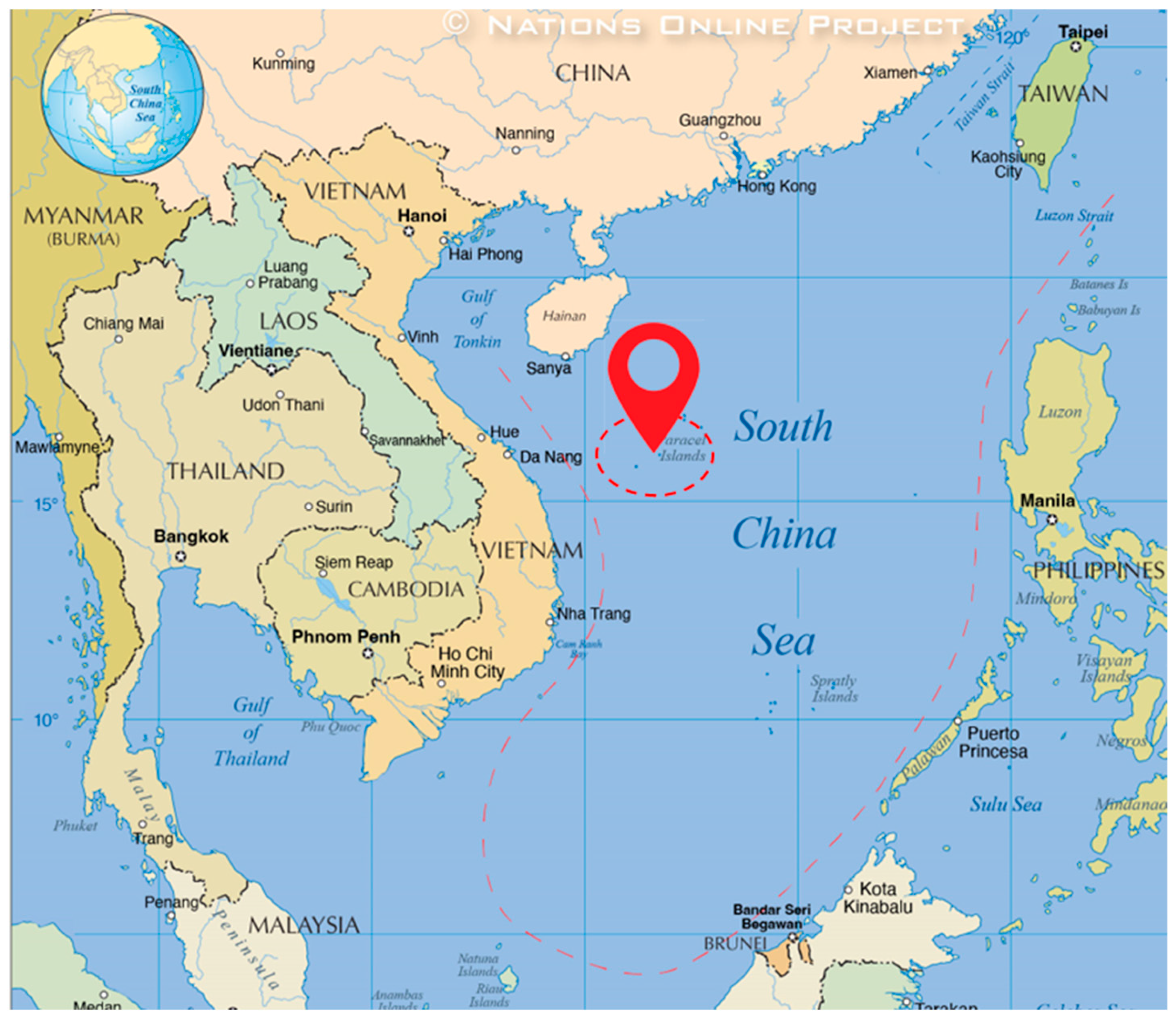
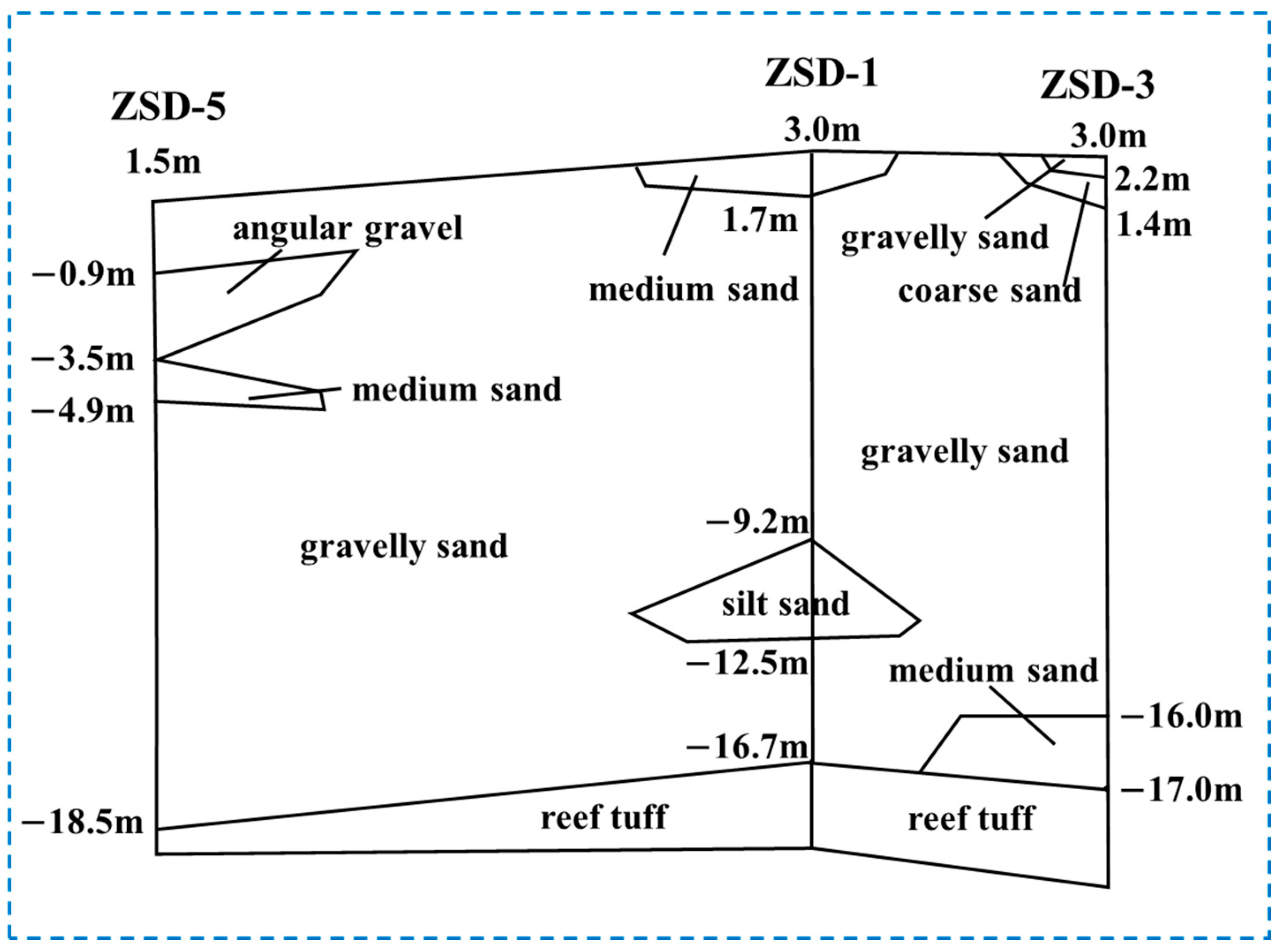
2.1. Overview of the Study Area

The study area is an island in the South China Sea, situated at 16°59′ N latitude and 112°16′ E longitude, with its geographical location depicted in Figure 1. This island belongs to China and is located in the northwestern waters of the South China Sea; it is a typical instance of expanding land area through blowing and filling on a natural reef. After blowing and filling, it has a land area of approximately 0.29 square kilometers and a vegetation coverage of around 60%. The island’s coast is divided into the primary coast and the later blown-in artificial coast. The primary coast is distributed in the northeast, east, and southeast of the island, while the later blown-in coast is distributed in the northwest, west, and southwest. The later blown-in coast is equipped with wave-protection dykes and stones thrown outside the dyke. The wave protection dyke comprises two types, i.e., dry-laid blocks and mortar-laid blocks, and the slope of the dyke surface ranges from 50 to 60 degrees. Geological boreholes, namely, ZSD-1, ZSD-3, and ZSD-5, were drilled on the island’s center, inner coast, and outer coast, respectively. When these boreholes were drilled to a certain depth within the reef tuff layer, the depth was taken as the ultimate standard. Based on the drilling data, the stratigraphic generalization model of the island, as presented in Figure 2, reveals that the underground water-bearing medium of the island has a binary structure, that is, a coral sand layer and a reef tuff layer. In the coral sand layer, the majority consists of gravelly sand, with a small amount of silt, medium sand, coarse sand, and angular gravel distributed locally. The interface between the coral sand layer and the reef tuff layer is an unconformable interface existing 16.7 to 18.5 m below the ground surface, so the numerical simulation part of this paper also adopts this binary aquifer structure. According to an on-site water quality survey, the salinity and conductivity of the nearshore seawater of the island are relatively stable and only fluctuate within a narrow range, with the salinity varying within the range of 35.5 to 36 and the conductivity varying within the range of 54,000 to 54,750 microsiemens/cm. The overall salinity of the seawater in the waters surrounding the coral islands and reefs, both nearshore and offshore, does not change significantly. However, the concentration of chloride ions in the seawater slightly increases as it moves away from the islands and reefs.

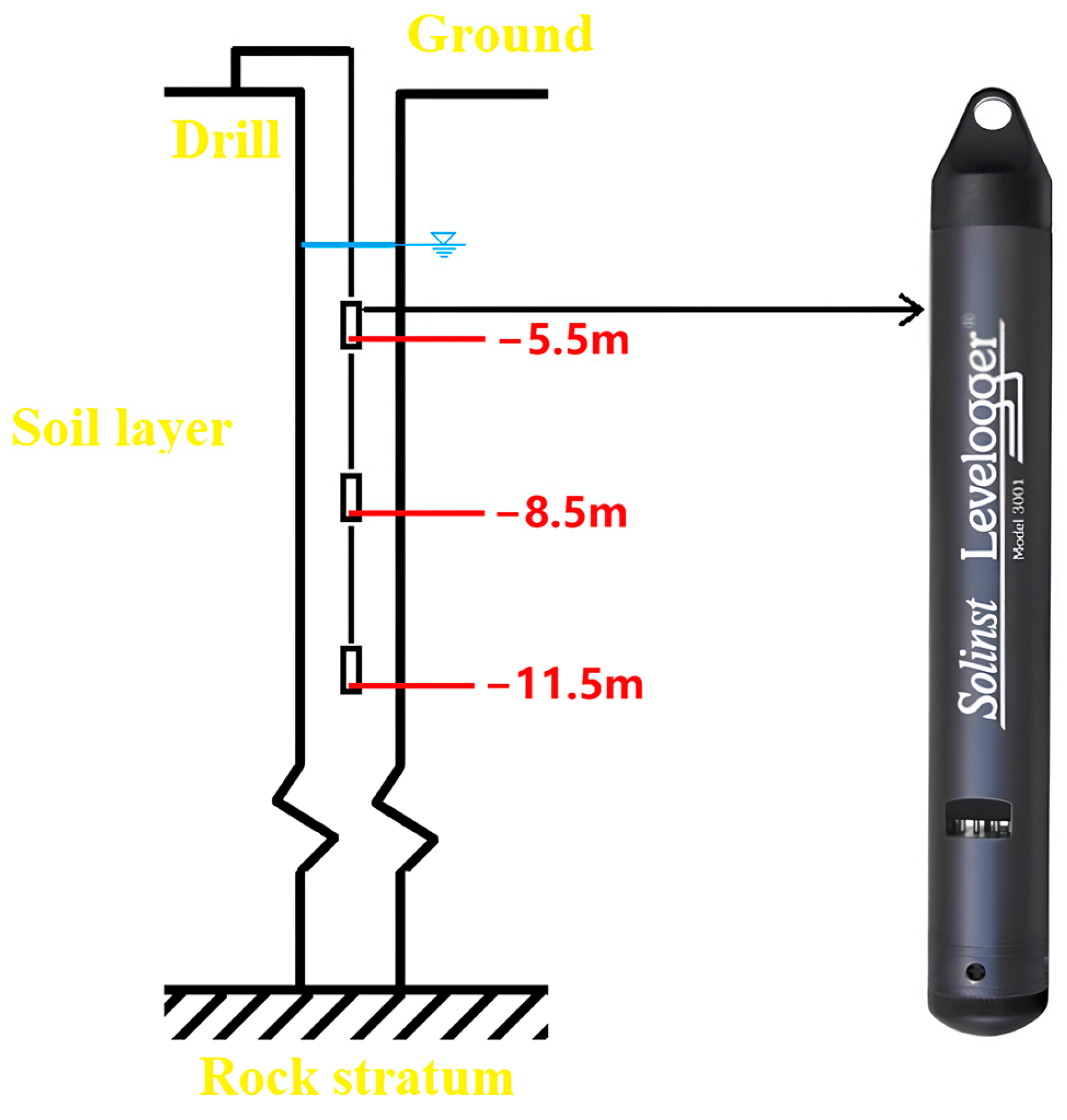
2.2. Water Quality Observation Methods

To ensure the principle of ecological and environmental protection of the island, large-scale geological exploration work on the island should be avoided as much as possible. Therefore, in line with the principle of fewer holes, while still revealing the hydrogeological conditions of the island as much as possible, three hydrological monitoring wells were installed at the locations of the previous geological boreholes. To prevent the borehole walls from collapsing and being clogged by fine particles, a 90 mm diameter PVC perforated pipe with a 3 mm diameter hole was placed in the boreholes. There was a series of holes on the pipe wall with a 10 cm interval between the vertical holes. Additionally, a layer of geotextile was wrapped around the PVC pipe to ensure that the groundwater in the borehole could exchange with the surrounding groundwater and that excessive fine soil particles would not enter the borehole, which could lead to clogging. After the groundwater in the boreholes had rested sufficiently, observation sensors were placed at depths of 5.5 m, 8.5 m, and 11.5 m in the three hydrological monitoring wells to record groundwater information throughout the day. Sensors were also placed in the island’s tide station to record tidal data. The frequency of equipment calibration and external data recovery was once a quarter, and professional engineers were responsible for removing anomalies by comparing and analyzing the data collected at each monitoring site. The remaining data were taken as the site’s final monitoring data. The water quality monitoring sensor employed the LTC Levelogger three-parameter groundwater logger manufactured by the Canadian company Solinst. This sensor has a built-in microcomputer and battery and can automatically record groundwater level, conductivity, and temperature data offline. The data collection interval of the water quality monitor is 5 min, a 24 h day, and the maximum operating time is 8 years. A schematic diagram of the sensors and their arrangement is shown in Figure 3. The authors installed a small weather station on the island to obtain meteorological data synchronized with the water quality monitoring data. The weather station system encompasses a data collector, an air temperature and humidity sensor, a wind speed and direction sensor, a photosynthetically active radiation sensor, a total radiation sensor, a precipitation sensor, a soil three-parameter sensor, and a soil heat flux sensor. The weather station collected data every 15 min, and the observation period was from January to December 2018.

3. Study on Freshwater Lens Simulation

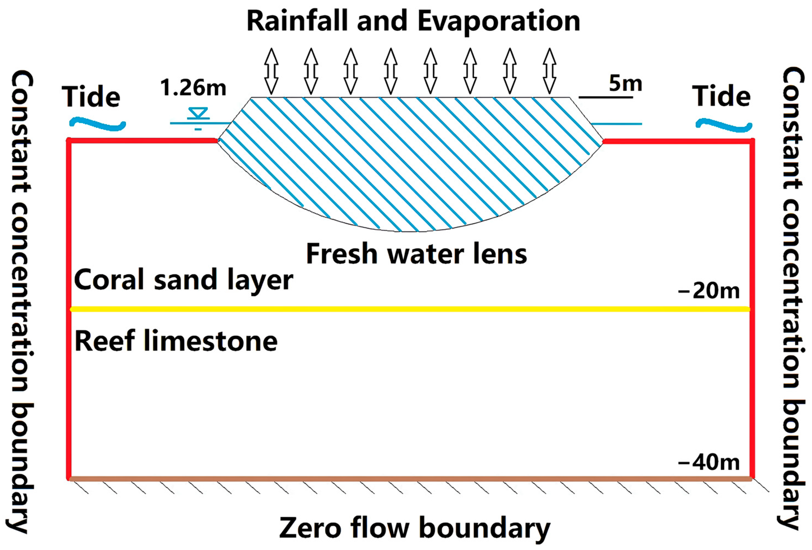
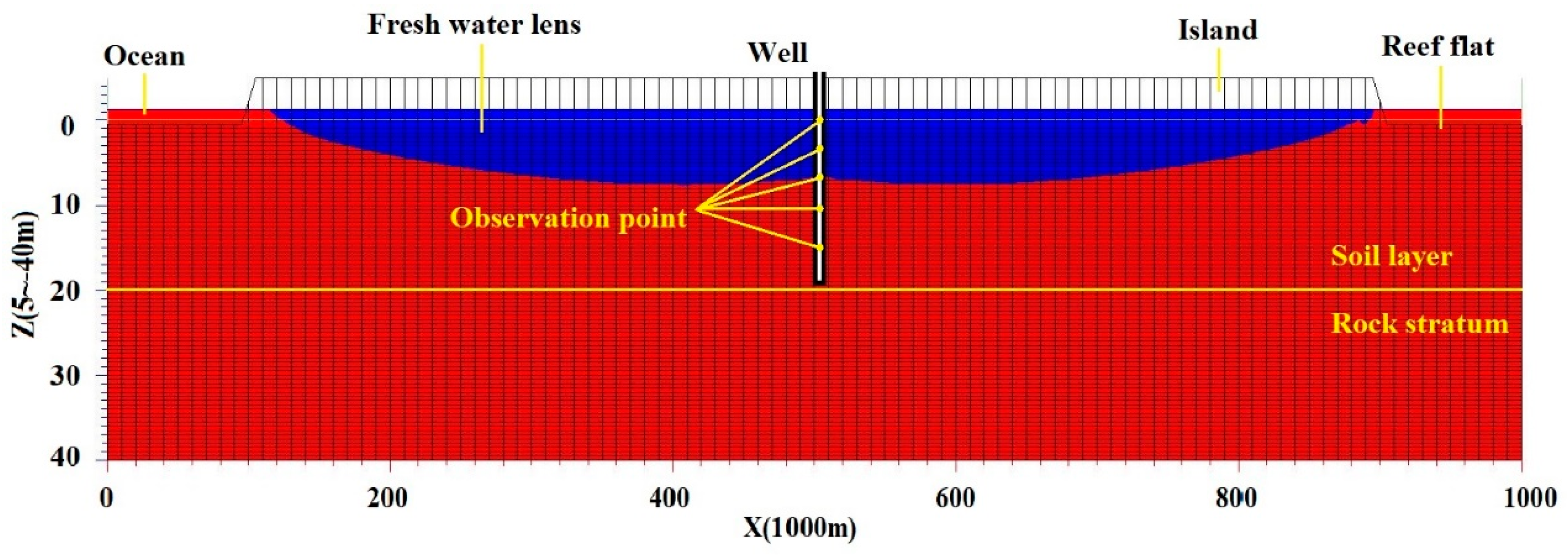
3.1. Model Construction

Numerical simulation was performed to investigate the impact of precipitation and tides on the freshwater lens, as well as the impact of the minimum boundary time scale on the simulated properties of the freshwater lens. Given that this study was focused on tides, precipitation, and time scales, the impact of the strata was ignored. Accordingly, the classic binary geological structure of islands was adopted in this study. Previous drilling results showed that the interface in the binary structure was at an elevation of −20 m [22,23,24]. A conceptual diagram is shown in Figure 4. The raised part in the middle was a coral island above sea level, and the low-lying parts on both sides of the island were reef flats.

3.2. Selection of Basic Parameters of the Model

A conceptual model was established in which the tidal level and effective precipitation recharge were set to fixed values in the boundary conditions. According to the observation data of the coral reef island from January to December 2018, the annual mean tidal elevation was 1.26 m, and the precipitation recharge rate was 0.003722 m/d. In particular, many factors should be considered when setting the precipitation recharge rate, such as evaporation, plant transpiration, capillary action, and the water-holding capacity of the soil layers. According to previous studies, the effective infiltration coefficient was set to 0.6 [25,26].

3.3. Setting of Model Boundary Conditions

The basic model information is summarized in

Table 1. Basic model information.

Model Information	Description
Model elevation	−40 m to 5 m
Model horizontal size	1000 m
Stratum structure	5 to −20 m: coral soil layer; −20 to −40 m: reef limestone layer
Hydrogeological parameter	Specific yield: 0.25; dispersity: 5 m; porosity: 0.3; elastic storativity: 0.00001
	Permeability coefficient: 100 m/d (calcareous soil layer); 1500 m/d (reef limestone layer)
Boundary conditions	Reef platform surface boundary and stratum lateral boundary: fixed concentration (19 g/L) and fixed water level boundary (1.26 m)
	Top boundary of the reef: fixed-supply boundary (0.003722 m/d); model bottom boundary: zero-flow boundary
Initial conditions	Initial water level: 1.26 m
	Initial concentration: 19 g/L below the initial water table, and 0 above the initial water level
Mesh	100 layers vertically; 90 layers horizontally
Time discretization	1 stress period, for a total of 10,800 days

. When investigating the impact of precipitation on the freshwater lens, the fixed-supply boundary condition was changed to the variable-supply boundary condition. The rainfall recharge data were measured on-site on the coral reef island from January to December 2018. When investigating the impact of tides on the freshwater lens, the fixed-water-level boundary condition was changed to the variable-water-level boundary condition. The water level was measured on-site on the coral reef island from January to December 2018. When investigating the impact of the boundary time scale on the simulation results of the freshwater lens, it was necessary to adjust the boundary conditions for temporal discretization, supply, and water level. When performing simulation under boundary conditions at a monthly scale, each stress period was set to 30 days for 360 stress periods, totaling 10,800 days (30 years) as the simulation duration; the boundary supply was set to the monthly mean supply, and the boundary water level was set to the monthly mean water level. When performing simulation under boundary conditions at the daily scale, each stress period was set to 1 day for 10,800 stress periods, totaling 10,800 days (30 years) as the simulation duration; the boundary supply was set to the daily mean supply, and the boundary water level was set to the daily mean water level. When performing simulation under boundary conditions at the hourly scale, each stress period was set to 0.0417 days for 259,200 stress periods, totaling 10,800 days (30 years); the boundary supply was set to the hourly mean supply, and the boundary water level was set to the hourly mean water level. The measured precipitation recharge and tidal water level at different time scales on the coral reef island from January to December 2018 are shown in Figure 5 and Figure 6, respectively.

3.4. Principle of Model Calculation

Freshwater lenses are special groundwater bodies formed jointly by solute transport and convection. For freshwater lens formation in coral islands, two equations (variable-density current equation and solute transport equation) can be solved simultaneously to simulate the formation process of lens bodies in real conditions. In Groundwater Modeling System (GMS10.8) software, the flow and transport simulators MODFLOW (GMS10.8) and MT3DMS (GMS10.8) are coupled by the SEAWAT (GMS10.8) module based on the synchronization of stress periods. The governing equations are as follows [27,28]:

(1) The water flow equation is based on conservation of mass and Darcy’s law.

$$K\left({\displaystyle \frac{{\partial }^{2}H}{\partial x^2}}+{\displaystyle \frac{{\partial }^{2}H}{\partial y^2}}+{\displaystyle \frac{{\partial }^{2}H}{\partial z^2}}\right)+K\eta {\displaystyle \frac{\partial c}{\partial z}}=S_s{\displaystyle \frac{\partial H}{\partial t}}+n\eta {\displaystyle \frac{\partial \mathrm{c}}{\partial \mathrm{t}}}-{\displaystyle \frac{\rho }{{\rho }_0}}{q}_s$$

(1)

In the above formula, K is the permeability coefficient, in m/d; η is the density coupling coefficient, in kg/m³; H is the hydraulic head, in m; n is the porosity of the porous medium; x, y, and z are coordinates; S_s is the specific storage of the porous material; t is time, in d; c is the concentration of the mixed fluid, in kg/m³; ρ is the density of the mixed fluid, in kg/m³; and q_s is the volumetric flow rate of sources or sinks per unit volume of the porous medium, in d⁻¹.

(2) The solute transport equation is used to describe the process of solute transport.

$${\displaystyle \frac{\partial \mathrm{c}}{\partial \mathrm{t}}}+u_i\left({\displaystyle \frac{\partial \mathrm{c}}{\partial x_i}}\right)={\displaystyle \frac{\partial }{\partial x_i}}\left(D_{ii}{\displaystyle \frac{\partial \mathrm{c}}{\partial x_i}}\right)+{\displaystyle \frac{c^{*}-c}{n}}{q}_s$$

(2)

In the above formula, $c^{*}$ is the concentration of fluid produced by sources or sinks, in kg/m³; t is time, in d; n is the porosity of the porous medium; c is the concentration of the mixed fluid, in kg/m³; q_s is the volumetric flow rate of sources or sinks per unit volume of the porous medium, in d⁻¹; x, y, and z are coordinates; $u_i$ is the penetration rate, in m/d; and D_ii is the dispersion coefficient, in m²/d.

3.5. Conversion Relations and Simulation Schemes

Two commonly used parameters to characterize groundwater quality of coral islands are conductivity and salinity. To facilitate data analysis, two mathematical relationships between the observed conductivity and salinity were comparatively established (Figure 7). The quadratic relationship (Figure 7a) has a goodness-of-fit (R2) of 1, and thus, such a relationship can be used for conversion between conductivity and salinity. The linear relationship (Figure 7b) has an R2 of 0.9986. Despite its relatively lower R2, the linear relationship is mathematically simple and can be used as a rapid, on-site conversion tool.

The simulation scheme is shown in

Table 2. Simulation scheme.

No.	Rainfall Supply	Tidal Water Level
a	Uniform	Uniform
b	Monthly changing	Uniform
c	Uniform	Monthly change
d	Monthly changing	Monthly change
e	Daily changing	Daily change
f	Hourly changing	Hourly change
Simulated time: 10,800 days

. A joint analysis of the simulation results of groups a, b, c, and d were used to reveal the effect mechanism of precipitation and tides on the formation of the freshwater lens. A joint analysis of groups d, e, and f was used to reveal the effect of boundary time scales on the simulated properties of the freshwater lens.

4. Study on the Response of Island Groundwater to Rainfall and Tides

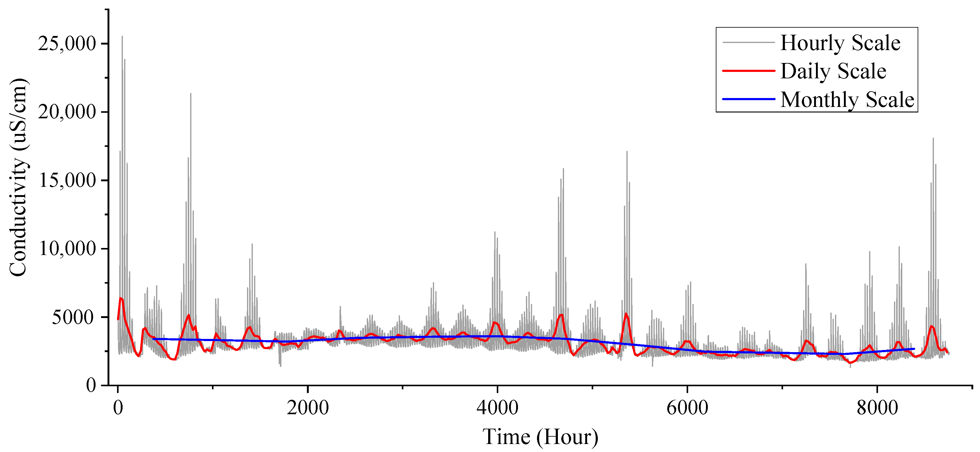
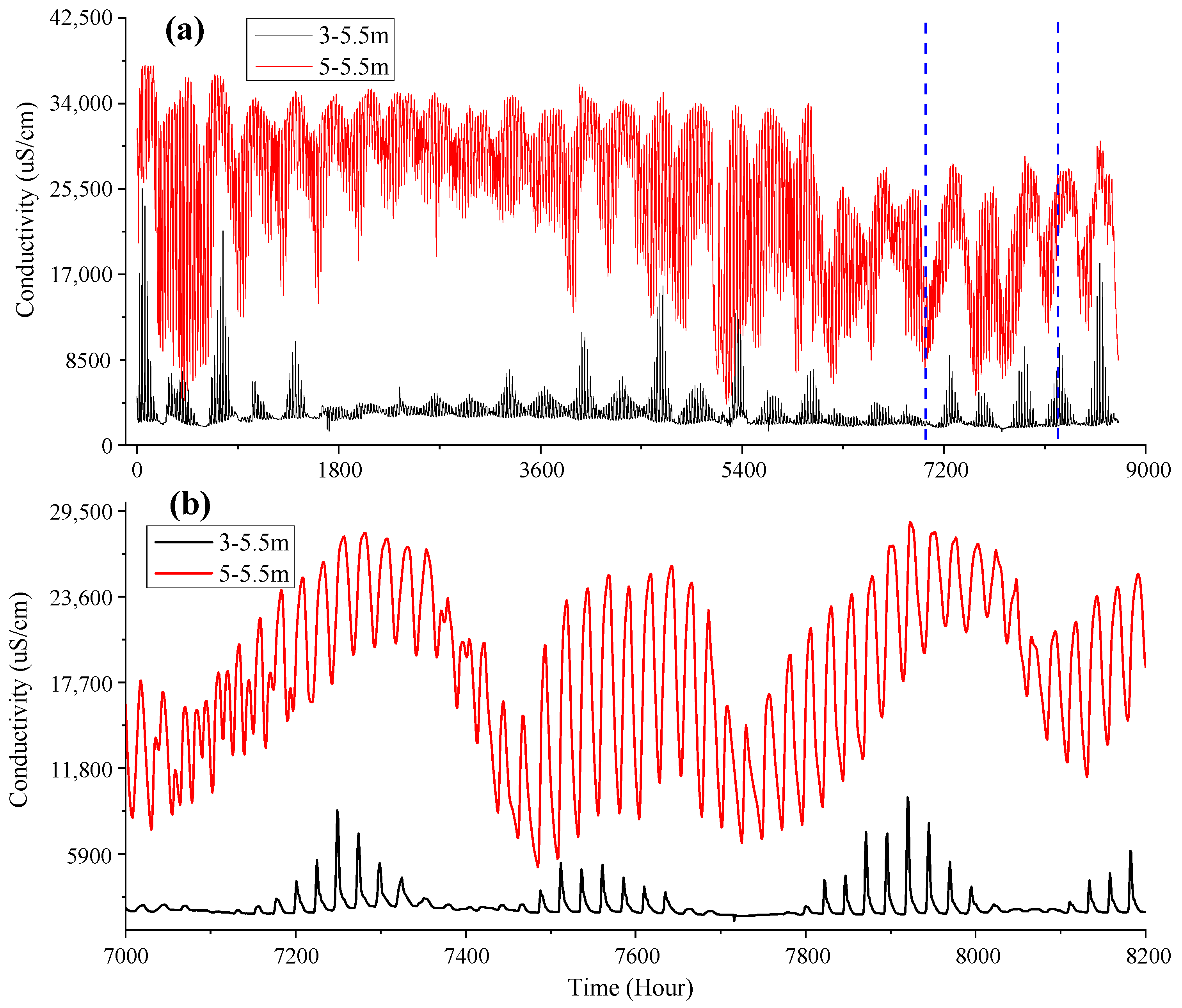
4.1. Study on Conductivity Response of Island Groundwater

Meteorological station data were collected every 15 min, and water quality data were collected every 5 min. Hourly, daily, and monthly scales were used separately in this study and were calculated separately for the mean groundwater level and conductivity and for cumulative precipitation. Figure 8 presents the time series of the precipitation and tidal level of the coral reef island with the time series of conductivity at a depth of 5.5 m in the ZSD-3 borehole of the island for the three time scales from January to December 2018.

In Figure 8, panels (a), (b), and (c) refer to the monthly, daily, and hourly scales, respectively. As shown in Figure 8, the monthly scale more clearly reveals the overall trends of conductivity, precipitation, and tidal level than the daily and hourly scales. That is, the conductivity and water quality at a fixed site on the coral island vary in the same direction as precipitation and the tidal level, indicating a general synchronization between conductivity, precipitation, and tidal level. As shown by the hourly series (Figure 8c), the conductivity shows a periodic fluctuation pattern resembling a normal distribution and is basically synchronized with the tidal level, indicating that the tidal level affects the period of fluctuation of groundwater conductivity. The plotted hourly series from 6297.6 h to 7237.4 h are shown in detail in Figure 9. The two green circles indicate the hours in which the precipitation is low and the peak conductivity is low; in contrast, the peak conductivity is high at the hours in which the precipitation is high and concentrated. This indicates that the precipitation affects the peak value of groundwater conductivity at the hourly scale. In Figure 8b, the overall trends of conductivity, precipitation, and tidal level can be observed, and there is a certain degree of periodic fluctuation in the data, but the trends and fluctuation patterns are less clear than those in Figure 8a,c. To more clearly compare the variation patterns in conductivity at the three time scales, the three time series of conductivity were plotted together (Figure 10).

As shown in Figure 10, different time scales lead to different variation patterns. The curve at the monthly scale clearly reveals the overall trend of groundwater conductivity, whereas the curve at the hourly scale shows the periodicity and peak values of groundwater conductivity in detail. The curve at the daily scale is similar to the curve at the hourly scale in terms of the data distribution pattern in each variation period; the overall trend at the monthly scale is synchronized with the direction of the curve at the daily scale. Meteorological observations often require analysis of a huge number of data at time scales of years and even decades; thus, it is necessary to select an appropriate time scale when processing and analyzing data for a specific research objective. If the objective is to reveal the overall trend of the data, the monthly scale can be used, whereas if the main objective is to investigate the periodicity of the data, the hourly scale may be a good choice. If both objectives are to be fulfilled simultaneously, the daily scale may be used.

Figure 11 is a scatter plot of conductivity versus water level at depths of 5.5 m, 8.5 m, and 11.5 m in the ZSD-3 borehole of the coral reef island from January to December 2018. The conductivity at the depth of 5.5 m varies between 2500 and 5000 μS/c for a water level below 1.1 m, but it rises sharply for a water level above 1.1 m. At the depth of 8.5 m, the conductivity varies between 300 and 5500 μS/cm for water levels below 1 m, but it rises sharply when the water level is above 1 m. At the depth of 11.5 m, there is a diffuse relationship between the conductivity and the water level, with fluctuation in the water level leading to sharp changes in conductivity. The above observations show that the groundwater sensors at depths of 5.5 m and 8.5 m below the ground surface are inside the freshwater lens throughout nearly all of the water-level fluctuation period, whereas the sensor at the depth of 11.5 m is transiently inside the freshwater lens when the water level is low and outside the freshwater lens at other times. These phenomena indicate that the entire freshwater lens moves vertically with the change in the tidal level because of the difference in density.

Figure 12 presents the hourly series of conductivity at the depth of 5.5 m in the ZSD-3 and ZSD-5 boreholes of the coral reef island from January to December 2018, with panel (a) partially zoomed-in and shown as panel (b). The figure indicates that groundwater conductivity is larger in the ZSD-5 borehole than in the ZSD-3 borehole, and the conductivity fluctuation patterns of the two holes are different, that is, the conductivity fluctuation pattern of the ZSD-5 borehole is more similar to that of the tidal level. This observation suggests that on a coral island, the closer to the shoreline, the higher the groundwater chloride concentration, and the greater the impact of tides on the groundwater chloride concentration.

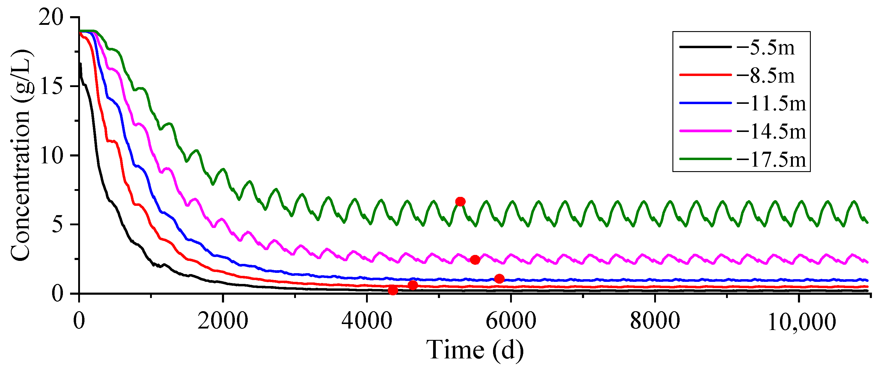
4.2. Simulation Study on the Influence of Rainfall and Tides on the Freshwater Lens

Because the present research objective was to reveal the effect mechanism of precipitation and tides on the formation of a freshwater lens rather than simulate and predict groundwater of actual coral islands, complicated stratigraphic factors were not considered in this study. Instead, the classic binary geological structure was adopted. To ensure the existence of a freshwater lens, the simulated island was set to 800 m in diameter and 100 m in the length of each reef flat on both sides. The boundary conditions were set by referring to the monitored tidal level and precipitation of the coral reef island from January to December 2018. The experimental scheme is shown in Table 2. In the following, simulation results and data acquisition methods are briefly explained by using group d in the experimental scheme as an example, while the simulation results of the other groups are directly presented without further elaboration on the acquisition process.

Figure 13 demonstrates the simulation result of group d (focused on monthly changes in precipitation and tides), in which the blue area is a steady-state freshwater lens, and the boundary chloride concentration of the lens was set to 1 g/L. An observation borehole was drilled in the center of the island, and borehole observation points were separately set at depths of 5.5 m, 8.5 m, 11.5 m, 14.5 m, and 17.5 m below the ground surface. Figure 14 demonstrates the daily series of the groundwater chloride concentration at each observation point during the whole simulation period, where the red dots represent the time points when the groundwater chloride concentration begins to stabilize, with the latest time point considered as the stabilization time point of the freshwater lens. The same procedure applies to the other experimental groups.

Figure 15, Figure 16, Figure 17 and Figure 18 demonstrate the simulated groundwater chloride concentration and water level in groups a, b, c, and d, respectively. Group a represents a simulation scenario of temporally invariant precipitation and tidal levels, group b represents monthly changing precipitation with temporally invariant tidal levels, group c represents temporally invariant precipitation with monthly changing tidal levels, and group d represents monthly changing precipitation and tidal levels.

Comparison of Figure 16a and Figure 17a with Figure 18a reveals that the curve shape of Figure 16a basically coincides with that of Figure 18a, while the curve shape of Figure 17a is relatively similar to that of Figure 15a. This observation indicates that during the formation of a freshwater lens, precipitation plays a dominant role in affecting groundwater chloride content, whereas changes in the tidal level have little effect on the desalination of groundwater in coral islands. Comparing Figure 16b and Figure 17b with Figure 18b reveals that the curve shape of Figure 17b basically coincides with that Figure 18b. This indicates that during the formation of a freshwater lens, the tidal level mainly affects the hydraulic head pressure at various points in the groundwater aquifer. The above results suggest that there is a remarkable difference between the effects of rainfall and tides on the freshwater lens [29], which is mainly manifested by the fact that rainfall directly introduces freshwater into the groundwater system through infiltration and dilutes salts, thereby significantly influencing the concentration of the groundwater. However, tides have a short fluctuation period, salt transport is controlled by dispersion, and the response time is extended, which makes it difficult for tides to alter the salt distribution of groundwater significantly; yet, because the density of seawater is higher than that of freshwater, tidal fluctuation directly affects the hydraulic gradient between seawater and groundwater, which in turn significantly affects the head pressure of groundwater.

Data on the stabilization time point, steady-state chloride concentration at the depth of 5.5 m below the ground surface, and groundwater hydraulic head level were extracted from Figure 15, Figure 16, Figure 17 and Figure 18, as presented in

Table 3. Simulation result summary for groups a–d.

Simulation Group	Stabilization Time Point (d)	Steady-State Concentration g/L	Steady-State Hydraulic Head (m)	Stabilization Time Point Error (%)	Steady-State Concentration Error (%)	Steady-State Hydraulic Head Error (%)
a	4717	0.0012	1.6739	19.66	99.43	0.42
b	5900	0.1449	1.6771	0.49	30.64	0.23
c	7000	0.054	1.6783	19.23	74.15	0.16
d	5871	0.2089	1.681	0.00	0.00	0.00

. Given that the boundary conditions of group d are the closest to the actual condition, the data of group d were subtracted from the data of other groups and then divided by the data of group d to give percent errors, as shown in Table 3. It can be observed that the rate of rainfall recharge determines the salt-driving efficiency; thereby, the time for the freshwater lens body to reach the steady state is significantly affected by rainfall. Not simulating rainfall variations leads to an error of 19.23%, while simulating only rainfall variations without tidal variations results in an error of only 0.49%. The steady-state chloride concentration of the freshwater lens is greatly affected by precipitation, that is, a failure to consider temporal precipitation changes results in a simulation error of 74.15%, whereas consideration of temporal precipitation changes but not temporal tidal-level changes results in a simulation error of 30.64%. As shown above, the groundwater hydraulic head of the steady-state freshwater lens is more affected by tides than precipitation. However, the head of the freshwater lens body is mainly driven by density differences [7], which leads to a relatively small attenuation of both effects on the steady-state head.

Figure 19 and Figure 20 demonstrate the simulation results of groups d, e, and f, with the three groups representing a simulation scenario of monthly, daily, and hourly changing precipitation and tidal levels, respectively. As shown in Figure 19, as the minimum time scale of a given set of boundary conditions increases, the water in the steady-state lens is desalinated to a greater extent. Under the same annual precipitation, the larger the minimum boundary time scale, the more uniform the precipitation, indicating that temporally invariant precipitation is conducive to the desalination of groundwater to form a freshwater lens, consistent with Panthi and Barkey et al. [20,30], who concluded that extreme weather harms freshwater lens formation on island reefs. As shown in Figure 20, with the elongation of the minimum time scale of a given set of boundary conditions, the steady-state groundwater hydraulic head of the island is higher, and thus more fresh groundwater is formed. Similarly, temporally invariant precipitation is more conducive to the formation of a freshwater lens. The stabilization time point of the freshwater lens, steady-state chloride concentration at the depth of 5.5 m, and steady-state head level were retrieved from Figure 19 and Figure 20, as shown in

Table 4. Simulation result summary for groups d–f.

Simulation Group	Stabilization Time Point (d)	Steady-State Concentration g/L	Steady-State Hydraulic Head (m)	Stabilization Time Point Error (%)	Steady-State Concentration Error (%)	Steady-State Hydraulic Head Error (%)
d	5871	0.2089	1.681	2.50	97.09	2.66
e	5862	1.2717	1.6773	2.34	82.29	2.44
f	5728	7.1812	1.6374	0.00	0.00	0.00

. Given that the boundary conditions of group f are most similar to the actual conditions, the data of group f were subtracted from the data of the other groups and then divided by the data of group f to give percent errors, as shown in Table 4.

As can be seen in Table 4, the larger the time scale, the greater the simulation error. Among them, the time scale has a relatively small impact on the time for the freshwater lens body to reach the steady state and the steady-state head, resulting in an error of only approximately 2.5%. The time scale significantly influences the concentration of the freshwater lens at the steady state, generating an error of 82.29% on the daily scale and 97.09% on the monthly scale. This outcome aligns with the response mechanism of freshwater lenses to rainfall and tides disclosed in the previous section. As depicted in Figure 8c, rainfall has a distinct multi-peak characteristic in the time scale map, which also drives synchronous oscillations in groundwater conductivity. As the time scale increases, such dynamic fluctuations are averaged into continuous recharge, leading to a remarkable difference in groundwater conductivity (the concentration of the freshwater lens) from the time scale at the steady state. In contrast, the steady-state time and head of the freshwater lens are mainly governed by the long-term equilibrium between rainfall recharge and groundwater discharge, and short-term tidal fluctuations only cause transient adjustments in the head [31], whose effect on the time for the freshwater lens to reach the steady state and the head is negligible.

5. Conclusions

Five main findings are achieved as follows:

(1)

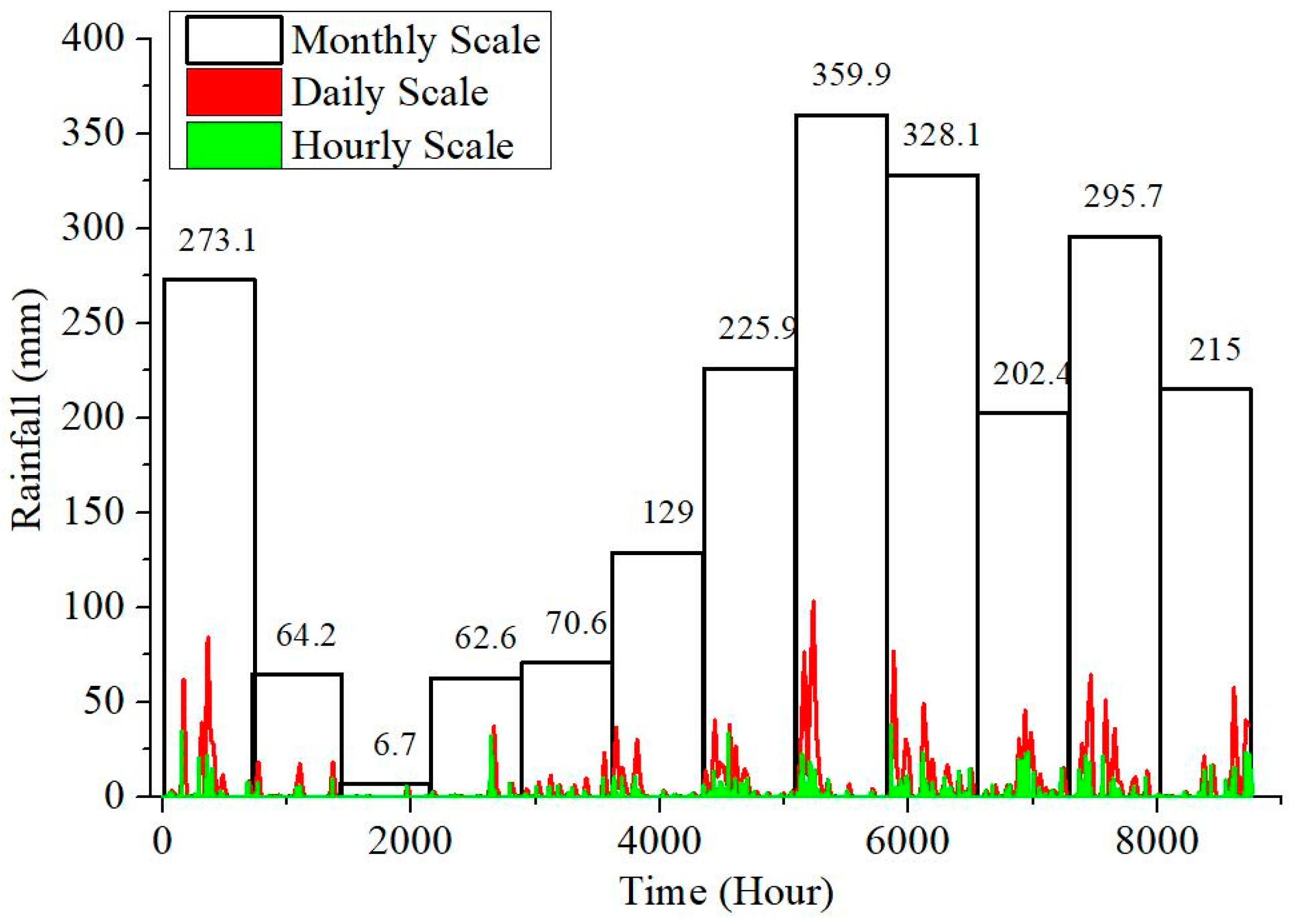
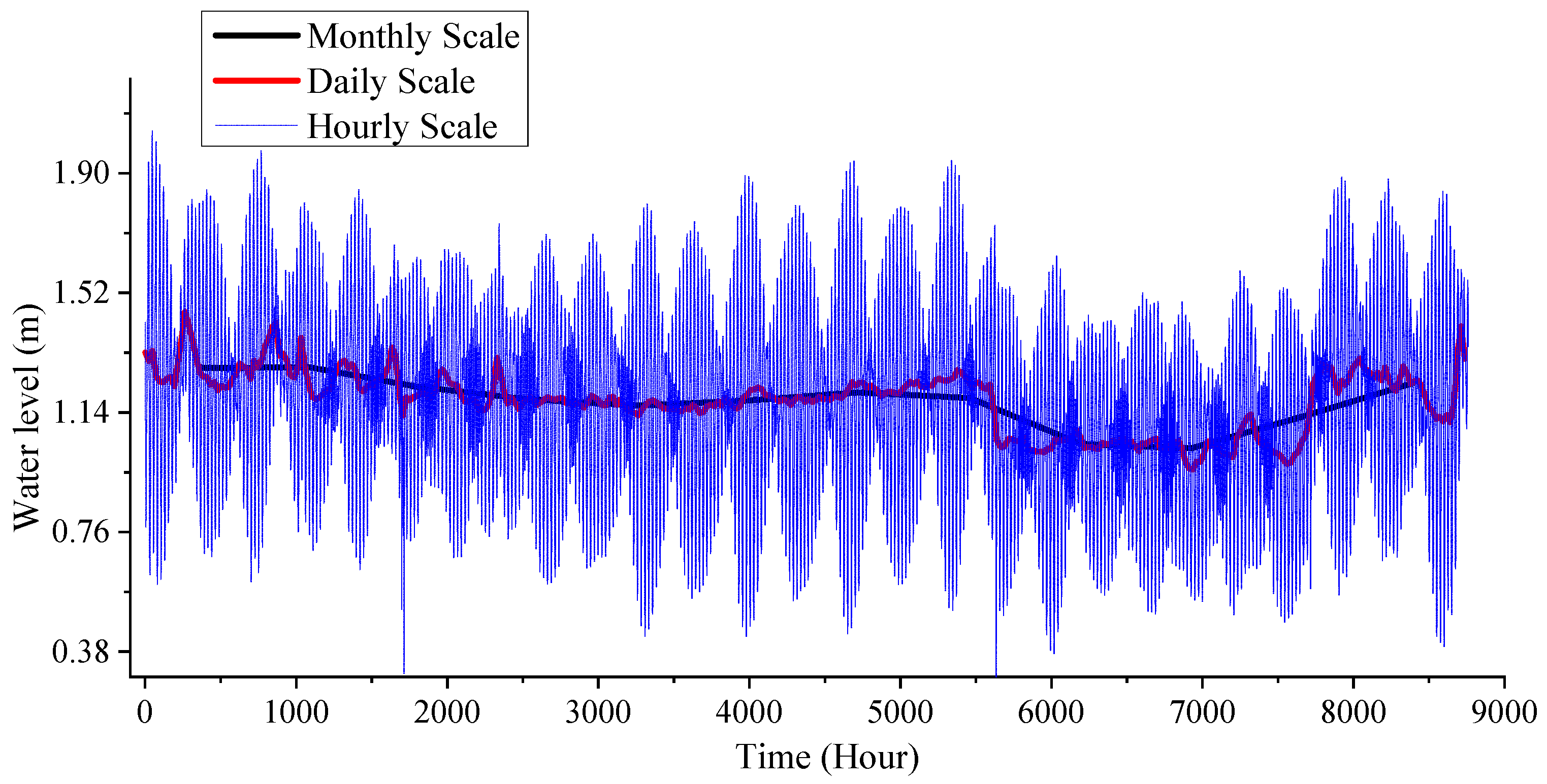
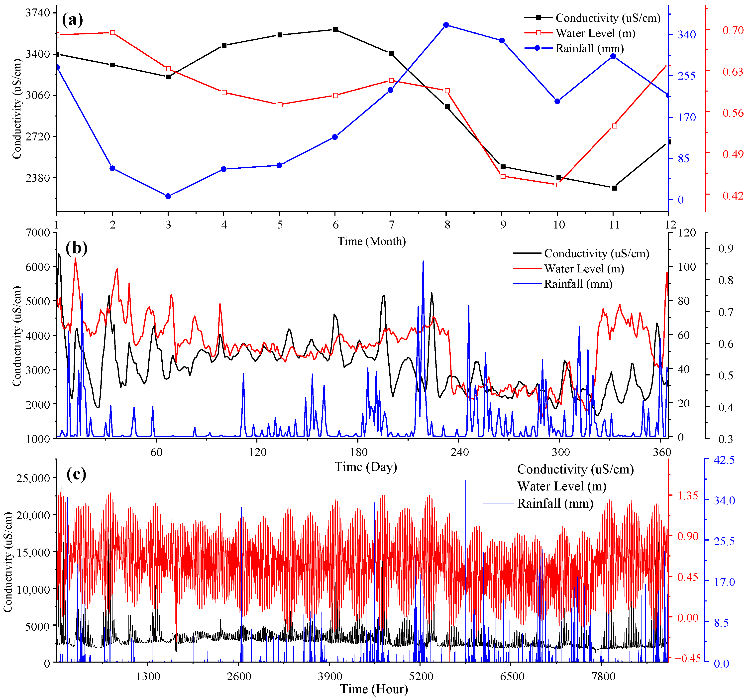
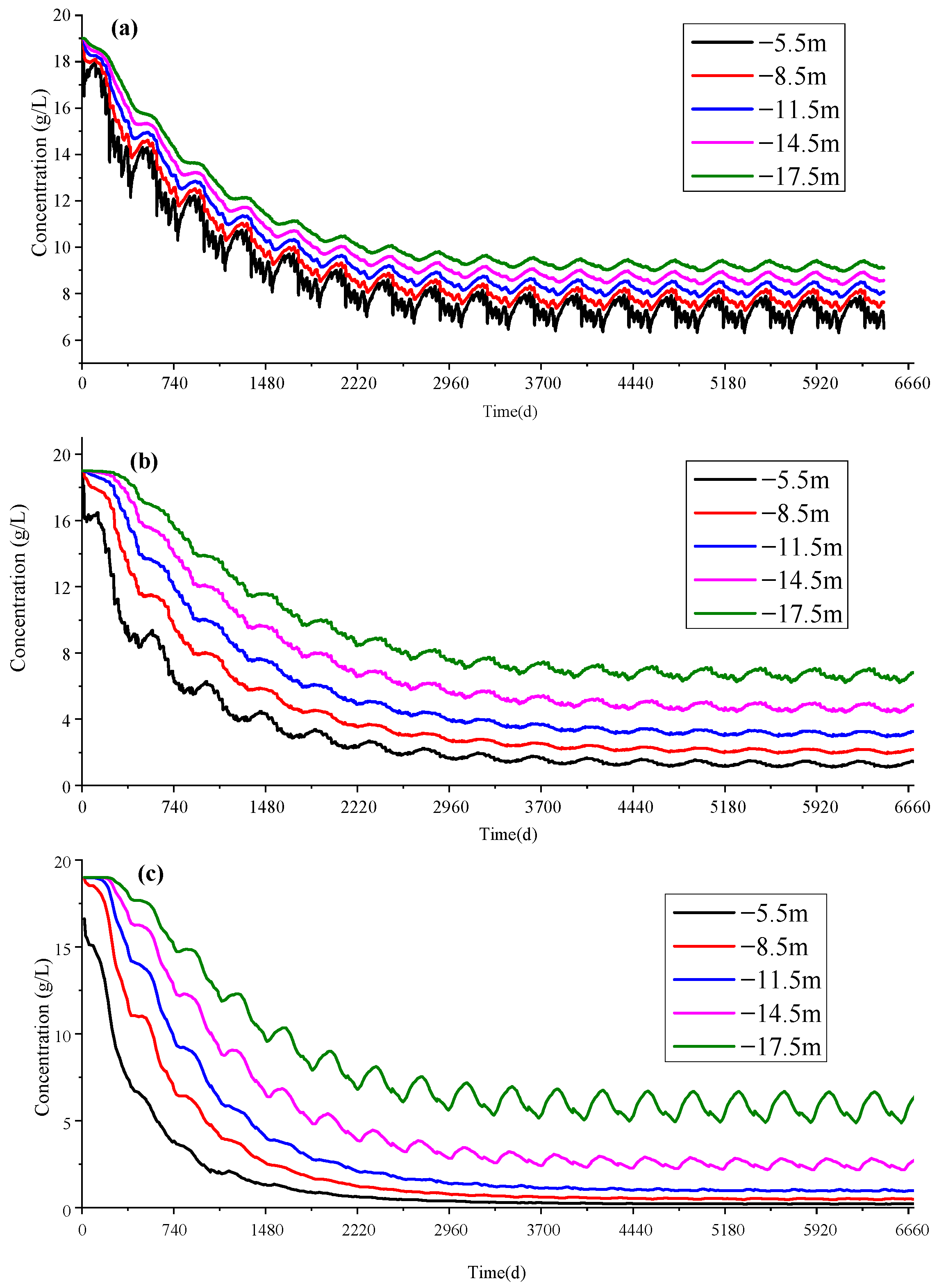
The groundwater conductivity of coral islands shows periodic fluctuation. Tidal level changes control the fluctuation periodicity of groundwater conductivity. The temporal distribution of precipitation controls the peak value of groundwater conductivity, with the peak value becoming higher as the precipitation becomes more temporally concentrated. The closer to the shoreline, the higher the chloride concentration of groundwater and the greater the impact of tides on the groundwater chloride concentration.

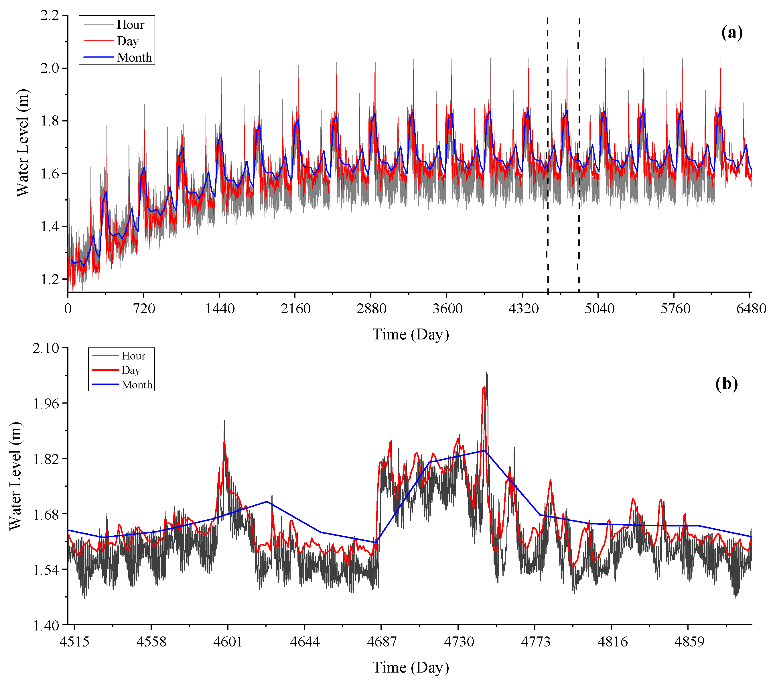
(2)

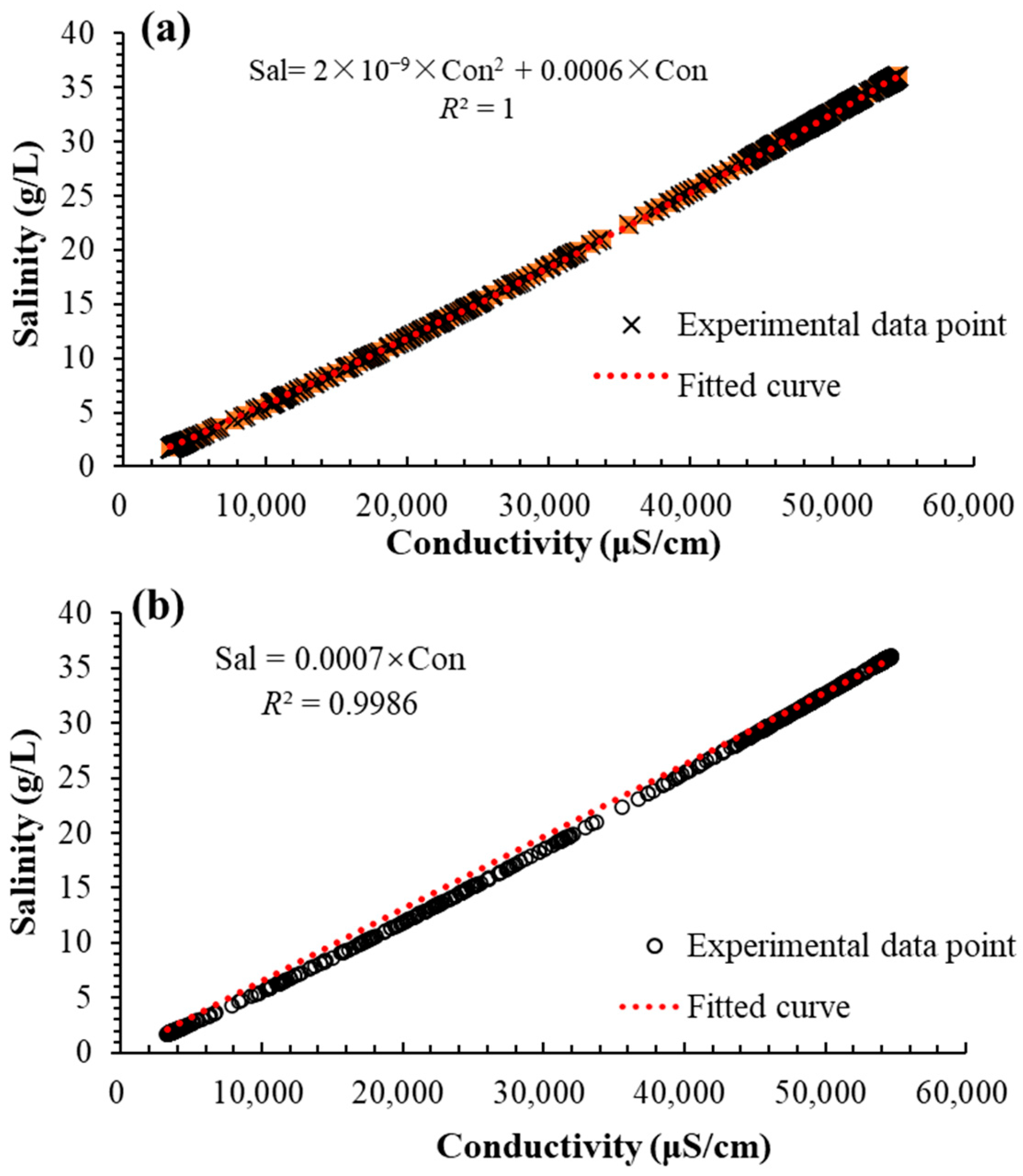
Observed data at different time scales have different usefulness. If the key issue to address is the overall trend of a freshwater lens, monthly observation data may be used. If the key issue to address is the periodicity in the changes in a freshwater lens, hourly observation data may be used. If the research focus is to investigate both simultaneously, daily observation data may be used. Moreover, an accurate conversion formula and fast conversion formula between seawater conductivity and salinity are obtained.

(3)

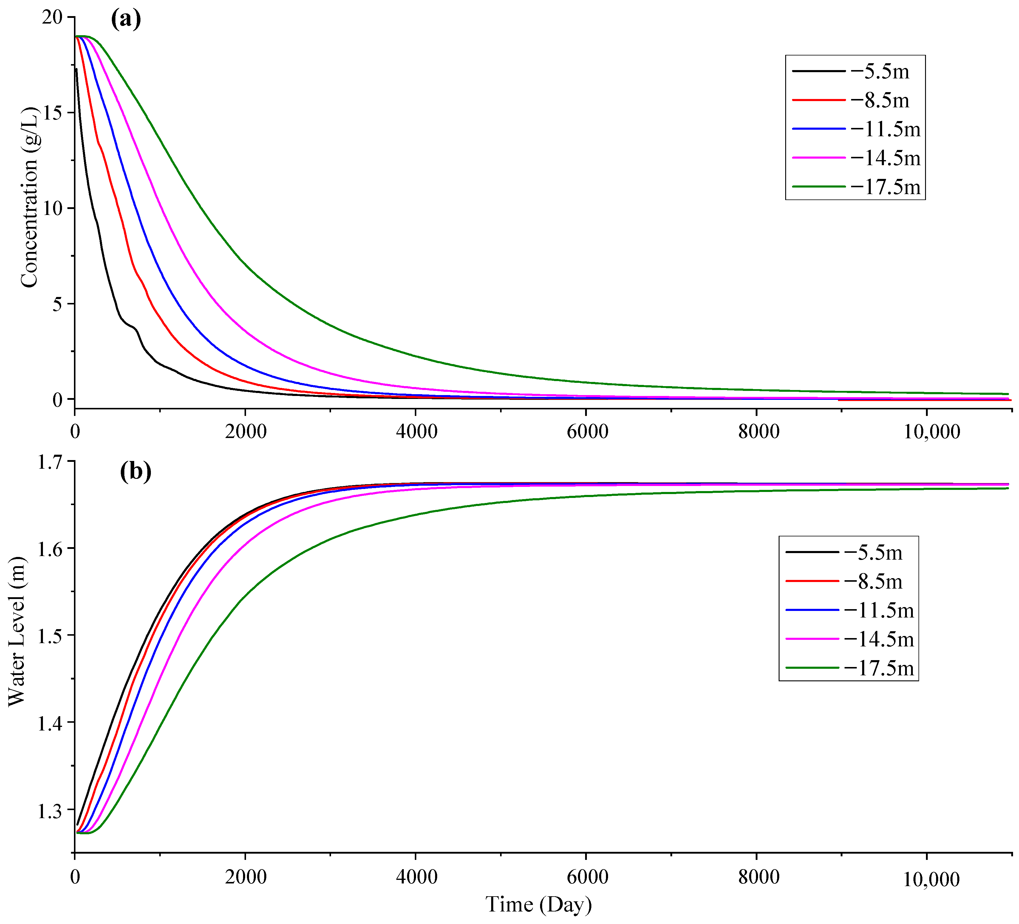
During the formation of a freshwater lens, precipitation mainly affects the chloride concentration of groundwater, whereas the tidal level mainly affects the groundwater hydraulic head pressure at various points in the groundwater aquifer.

(4)

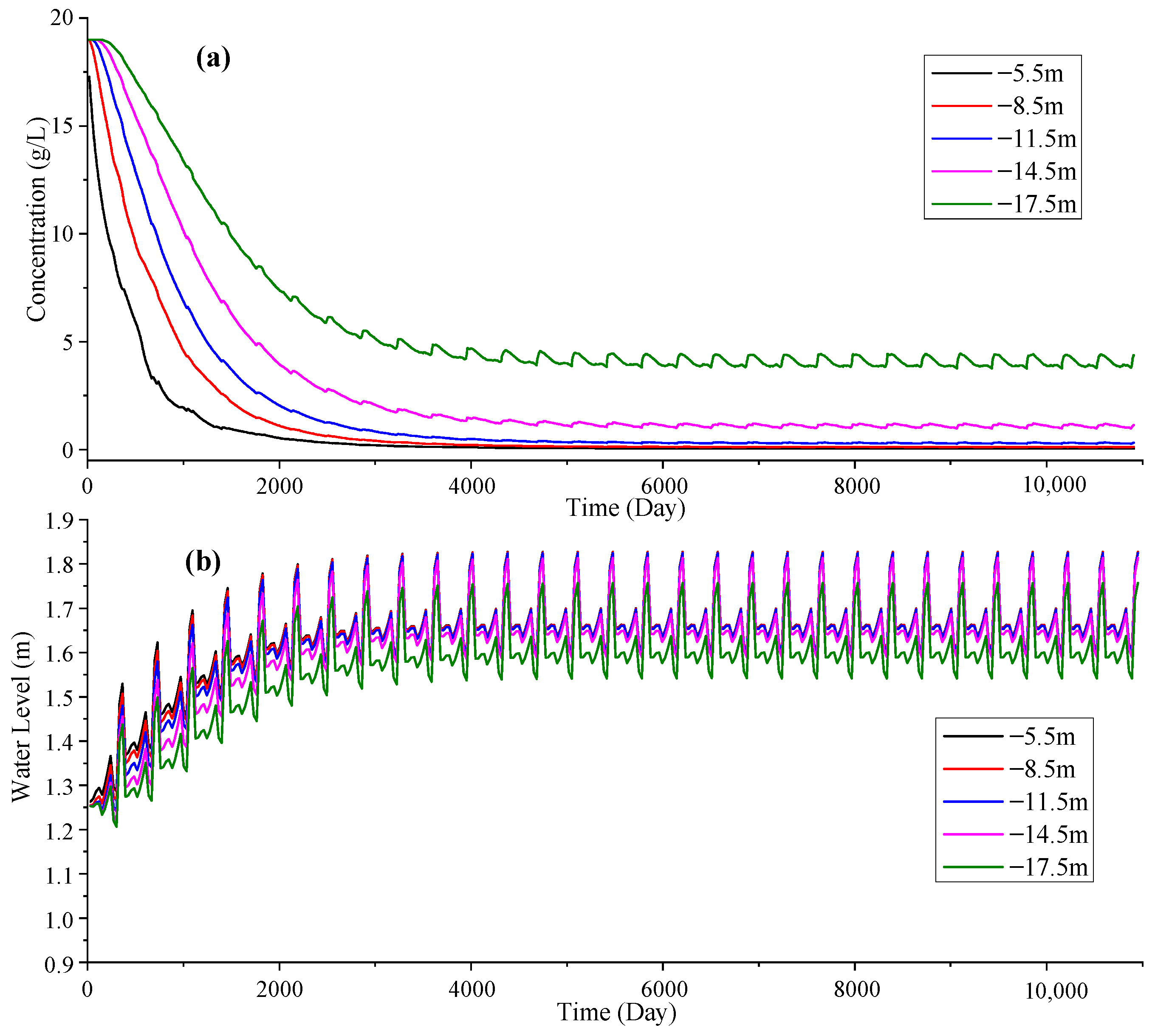
The stabilization time point and steady-state chloride concentration of a freshwater lens are mainly controlled by precipitation factors. The more temporally invariant the precipitation, the higher the desalination degree in the freshwater lens and the larger the freshwater storage. In the numerical simulation, a failure to consider temporal precipitation changes results in a simulation error of 19.23% and 74.15% in the stabilization time point and steady-state chloride concentration of the freshwater lens, respectively. The steady-state groundwater hydraulic head is more affected by tides than by precipitation, but neither has a great impact, with errors of only 0.16–0.23%.

(5)

The larger the minimum time scale of the boundary conditions in the numerical simulation, the greater the error in the simulation results. Time scales have little effect on the stabilization time point and steady-state hydraulic head of the fresh groundwater lens, with simulation errors of only about 2.5%. Time scales have a great impact on the steady-state chloride concentration of the freshwater lens, with simulation errors of 82.29–97.09% at the daily and monthly scales.

References

1. Zhao, M.X.; Yu, K.F.; Shi, Q.; Chen, T.R.; Zhang, H.L.; Chen, T.G. Coral Communities of the Remote Atoll Reefs in the Nansha Islands, Southern South China Sea. Environ. Monit. Assess. 2013, 185, 7381–7392. [Google Scholar] [CrossRef] [PubMed]
2. Wang, R.; Shu, L.; Zhang, R.; Ling, Z. Determination of Exploitable Coefficient of Coral Island Freshwater Lens Considering the Integrated Effects of Lens Growth and Contraction. Water 2023, 15, 890. [Google Scholar] [CrossRef]
3. Chui, T.F.M.; Terry, J.P. Influence of Sea-Level Rise on Freshwater Lenses of Different Atoll Island Sizes and Lens Resilience to Storm-Induced Salinization. J. Hydrol. 2013, 502, 18–26. [Google Scholar] [CrossRef]
4. Post, V.E.A.; Houben, G.J.; van Engelen, J. What Is the Ghijben-Herzberg Principle and Who Formulated It? Hydrogeol. J. 2018, 26, 1801–1807. [Google Scholar] [CrossRef]
5. Post, V.E.A.; Bosserelle, A.L.; Galvis, S.C.; Sinclair, P.J.; Werner, A.D. On the Resilience of Small-Island Freshwater Lenses: Evidence of the Long-Term Impacts of Groundwater Abstraction on Bonriki Island, Kiribati. J. Hydrol. 2018, 564, 133–148. [Google Scholar] [CrossRef]
6. Werner, A.D.; Sharp, H.K.; Galvis, S.C.; Post, V.E.A.; Sinclair, P. Hydrogeology and Management of Freshwater Lenses on Atoll Islands: Review of Current Knowledge and Research Needs. J. Hydrol. 2017, 551, 819–844. [Google Scholar] [CrossRef]
7. Vacher, H. Dupuit-Ghyben-Herzberg Analysis of Strip-Island Lenses. Geol. Soc. Am. Bull. 1988, 100, 580–591. [Google Scholar] [CrossRef]
8. Falkland, A. Hydrology and Water Management on Small Tropical Islands. In Hydrology of Warm Humid Regions; Gladwell, J.S., Ed.; International Association Hydrological Sciences: Wallingford, UK, 1993; pp. 263–303. [Google Scholar]
9. Werner, A.D.; Bakker, M.; Post, V.E.A.; Vandenbohede, A.; Lu, C.; Ataie-Ashtiani, B.; Simmons, C.T.; Barry, D.A. Seawater Intrusion Processes, Investigation and Management: Recent Advances and Future Challenges. Adv. Water Resour. 2013, 51, 3–26. [Google Scholar] [CrossRef]
10. Stoeckl, L.; Houben, G. Flow Dynamics and Age Stratification of Freshwater Lenses: Experiments and Modeling. J. Hydrol. 2012, 458–459, 9–15. [Google Scholar] [CrossRef]
11. Sonnenborg, T.O.; Hinsby, K.; van Roosmalen, L.; Stisen, S. Assessment of Climate Change Impacts on the Quantity and Quality of a Coastal Catchment Using a Coupled Groundwater-Surface Water Model. Clim. Change 2012, 113, 1025–1048. [Google Scholar] [CrossRef]
12. Schneider, J.C.; Kruse, S.E. Assessing Selected Natural and Anthropogenic Impacts on Freshwater Lens Morphology on Small Barrier Islands: Dog Island and St. George Island, Florida, USA. Hydrogeol. J. 2006, 14, 131–145. [Google Scholar] [CrossRef]
13. Underwood, M.; Peterson, F.; Voss, C. Groundwater Lens Dynamics of Atoll Islands. Water Resour. Res. 1992, 28, 2889–2902. [Google Scholar] [CrossRef]
14. Terry, J.P.; Falkland, A.C. Responses of Atoll Freshwater Lenses to Storm-Surge Overwash in the Northern Cook Islands. Hydrogeol. J. 2010, 18, 749–759. [Google Scholar] [CrossRef]
15. Chui, T.F.M.; Terry, J.P. Modeling Fresh Water Lens Damage and Recovery on Atolls After Storm-Wave Washover. Ground Water 2012, 50, 412–420. [Google Scholar] [CrossRef]
16. Chui, T.F.M.; Terry, J.P. Groundwater Salinisation on Atoll Islands after Storm-Surge Flooding: Modelling the Influence of Central Topographic Depressions. Water Environ. J. 2015, 29, 430–438. [Google Scholar] [CrossRef]
17. Comte, J.-C.; Banton, O.; Join, J.-L.; Cabioch, G. Evaluation of Effective Groundwater Recharge of Freshwater Lens in Small Islands by the Combined Modeling of Geoelectrical Data and Water Heads. Water Resour. Res. 2010, 46, W06601. [Google Scholar] [CrossRef]
18. Holt, T.; Greskowiak, J.; Seibert, S.L.; Massmann, G. Modeling the Evolution of a Freshwater Lens under Highly Dynamic Conditions on a Currently Developing Barrier Island. Geofluids 2019, 2019, 9484657. [Google Scholar] [CrossRef]
19. Jazayeri, A.; Werner, A.D.; Irvine, D.J. Transience of Riparian Freshwater Lenses. Water Resour. Res. 2022, 58, e2021WR031310. [Google Scholar] [CrossRef]
20. Panthi, J.; Boving, T.B.; Pradhanang, S.M.; Russoniello, C.J.; Kang, S. The Contraction of Freshwater Lenses in Barrier Island: A Combined Geophysical and Numerical Analysis. J. Hydrol. 2024, 637, 131371. [Google Scholar] [CrossRef]
21. South China Sea Map. Available online: https://ar.inspiredpencil.com/pictures-2023/south-china-sea-map (accessed on 20 March 2025).
22. Buddemeier, R.W.; Oberdorfer, J.A. Chapter 22—Hydrogeology of Enewetak Atoll. In Developments in Sedimentology; Vacher, H.L., Quinn, T.M., Eds.; Geology and Hydrogeology of Carbonate Islands; Elsevier: Amsterdam, The Netherlands, 2004; Volume 54, pp. 667–692. [Google Scholar]
23. White, I.; Falkland, T. Management of Freshwater Lenses on Small Pacific Islands. Hydrogeol. J. 2010, 18, 227–246. [Google Scholar] [CrossRef]
24. Ayers, J.; Vacher, H. Hydrogeology of an Atoll Island—A Conceptual-Model from Detailed Study of a Micronesian Example. Ground Water 1986, 24, 185–198. [Google Scholar] [CrossRef]
25. Singh, V.S. Evaluation of Groundwater Resources on the Coral Islands of Lakshadweep, India, 1st ed.; Springer: New York, NY, USA, 2016; ISBN 978-3-319-50072-0. [Google Scholar]
26. Jocson, J.M.U.; Jenson, J.W.; Contractor, D.N. Recharge and Aquifer Response: Northern Guam Lens Aquifer, Guam, Mariana Islands. J. Hydrol. 2002, 260, 231–254. [Google Scholar] [CrossRef]
27. Lin, J.; Snodsmith, J.B.; Zheng, C.; Wu, J. A Modeling Study of Seawater Intrusion in Alabama Gulf Coast, USA. Environ. Geol. 2009, 57, 119–130. [Google Scholar] [CrossRef]
28. Chen, K.R.; Chen, H.B.; Zhao, H.L. Numerical simulation of seawater intrusion based on SEAWAT. J. Water Resour. Water Eng. 2012, 23, 140–145. (In Chinese) [Google Scholar]
29. Oberle, F.K.J.; Swarzenski, P.; Storlazzi, C.D. Atoll Groundwater Movement and Its Response to Climatic and Sea-Level Fluctuations. Water 2017, 9, 650. [Google Scholar] [CrossRef]
30. Barkey, B.L.; Bailey, R.T. Estimating the Impact of Drought on Groundwater Resources of the Marshall Islands. Water 2017, 9, 41. [Google Scholar] [CrossRef]
31. Sheng, C.; Han, D.; Xu, H.; Li, F.; Zhang, Y.; Shen, Y. Evaluating Dynamic Mechanisms and Formation Process of Freshwater Lenses on Reclaimed Atoll Islands in the South China Sea. J. Hydrol. 2020, 584, 124641. [Google Scholar] [CrossRef]
Figure 1. Diagram of the location of the study area [21].
Jmse 13 00738 g001
Figure 2. Island stratigraphic information map.
Jmse 13 00738 g002
Figure 3. Sensors and deployment layout.
Jmse 13 00738 g003
Figure 4. Diagram of the conceptual model.
Jmse 13 00738 g004
Figure 5. Precipitation observation data at the three time scales.
Jmse 13 00738 g005
Figure 6. Tidal level curves at the three time scales.
Jmse 13 00738 g006
Figure 7. Conductivity–salinity relationship: (a) accurate conversion; (b) fast conversion.
Jmse 13 00738 g007
Figure 8. Conductivity, precipitation, and tidal level curves at the three time scales: (a) monthly scale; (b) daily scale; (c) hourly scale.
Jmse 13 00738 g008
Figure 9. Partial zoom-in of the plotted hourly series.
Jmse 13 00738 g009
Figure 10. Conductivity curves at the three time scales.
Jmse 13 00738 g010
Figure 11. Scatter plots of conductivity versus water level at different depths.
Jmse 13 00738 g011
Figure 12. Conductivity curves of different boreholes: (a) conductivity curves of the ZSD-3 and ZSD-5 boreholes; (b) partially zoomed-in view of (a).
Jmse 13 00738 g012
Figure 13. Simulation results of group d.
Jmse 13 00738 g013
Figure 14. Daily series of monitored chloride concentration of group d.
Jmse 13 00738 g014
Figure 15. Daily series of the simulated chloride concentration and water level of group a (temporally invariant precipitation and tides): (a) chloride concentration; (b) water level.
Jmse 13 00738 g015
Figure 16. Daily series of the simulated chloride concentration and water level of group b (temporally variant precipitation with temporally invariant tides): (a) chloride concentration; (b) water level.
Jmse 13 00738 g016
Figure 17. Daily series of the simulated chloride concentration and water level of group c (temporally invariant precipitation with temporally variant tides): (a) chloride concentration; (b) water level.
Jmse 13 00738 g017
Figure 18. Daily series of the simulated chloride concentration and water level of group d (temporally variant precipitation and tides). (a) Chloride concentration; (b) water level.
Jmse 13 00738 g018
Figure 19. Time series of the simulated chloride concentration of groups d, e, and f: (a) hourly scale; (b) daily scale; (c) monthly scale.
Jmse 13 00738 g019
Figure 20. Time series of the simulated water level of groups d, e, and f: (a) the three time scales; (b) partially zoomed-in view of (a).
Jmse 13 00738 g020