Abstract
The Sulu Sea has active internal tides (ITs) and basin-scale circulation. This study, for the first time, employs three-dimensional simulations to investigate the effects of the Sulu Sea circulation on IT generation and propagation. Results reveal that the cyclonic circulation can enhance the semi-diurnal and diurnal IT energy conversion in the Sulu Archipelago by approximately 17% and 77%, respectively, compared to those without circulation for semi-diurnal ITs (4.36 GW) and diurnal ITs (2.76 GW). This different increase portion between semi-diurnal and diurnal ITs is attributed to different influences of circulation on the positive and negative conversion rates for semi-diurnal and diurnal ITs. Energy budget analysis indicates that circulation increases the proportion of dissipation near source regions from 88% (90%) to 94% (93%) and reduces the proportion of energy flux radiation from 12% (10%) to 6% (7%) for semi-diurnal (diurnal) ITs. The ray-tracing results indicate that the cyclonic circulation induces significant westward refraction of IT rays by modulating IT speeds in counter-current/co-current regions. Further sensitive experiments reveal that circulation-induced stratification weakens the refraction, whereas the background currents strengthen it, with the latter dominating. These findings advance our understanding of the IT behaviors in the Sulu Sea under the modulation of circulation.
1. Introduction
Internal waves are a common phenomenon in the stratified ocean, with their largest amplitudes occurring below the surface and minimal surface expressions. Internal waves including internal solitary waves (ISWs) and internal tides (ITs) primarily result from the interaction between tidal currents and abruptly varying topography. Compared to nonlinear ISWs, ITs are linear internal waves, with periods corresponding to semi-diurnal or diurnal tidal cycles. These waves exhibit wavelengths ranging from tens to hundreds of kilometers and induce vertical isopycnal displacements on the order of tens of meters. ITs are ubiquitous in the global ocean, transporting energy from generation sites over distances of several hundred kilometers [1,2]. As a key driver of ocean mixing [3,4], ITs play a fundamental role in regulating oceanic energy distribution and influencing biogeochemical processes [5,6].
The Sulu Sea, located at the western edge of the Pacific Ocean (Figure 1), is surrounded by a chain of islands, including the Sulu Archipelago, Palawan Island, Mindanao Island, and Kalimantan Island. It connects to the South China Sea via the Balabac and Mindoro Straits in the north, to the Celebes Sea through the Sulu Archipelago in the south, and to the Pacific Ocean through the Surigao Strait in the east (Figure 1). This strategic location makes the Sulu Sea a vital pathway linking the Western Pacific, the South China Sea, and the Eastern Indian Ocean.
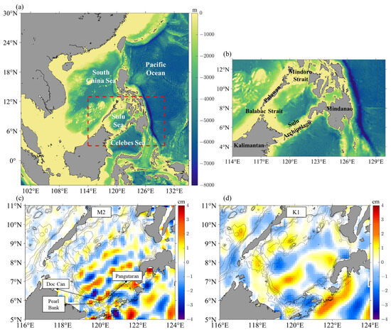
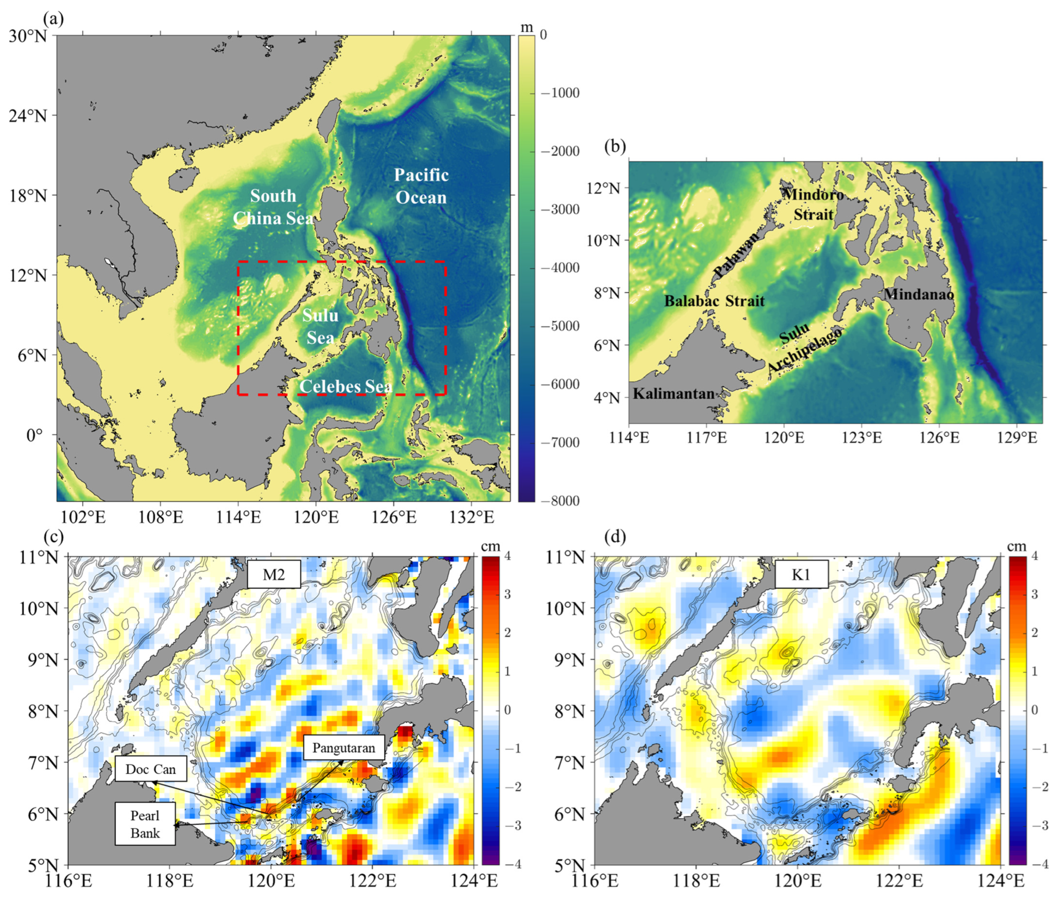
Figure 1.
(a) The bathymetry distribution in the range of 0–135° E, 5° S–30° N. (b) The bathymetry distribution around the Sulu Sea within the red box in (a). (c,d) The snapshots of SSH induced by M2 and K1 ITs, respectively, as derived from the MIOST-IT dataset. Bathymetry is contoured at depths by thin black lines of −100, −200, −500, −1000, and −2000 m.
The Sulu Sea is recognized as one of the most active regions for ISWs and ITs. In previous studies, these waves have been observed/investigated through remote sensing and in situ observations [7,8,9,10]. Previous studies have shown that the ITs in this region primarily originate from the interaction between barotropic tidal currents and abruptly varying topography in the southern Sulu Archipelago [9,10]. These ITs are predominantly semi-diurnal, with an estimated baroclinic energy conversion rate of 10.8 GW and a dissipation rate of −7.8 GW, indicating that a significant portion of the energy dissipates near the generation sites [9]. Using multi-year satellite altimetry data, Zhao et al. (2021) [10] estimated the northward semi-diurnal IT energy flux radiating from the Sulu Archipelago into the Sulu Sea to be approximately 0.46 GW.
In recent years, the interaction between ITs and circulation or mesoscale eddies has gained considerable attention [11,12,13]. Circulation and mesoscale eddies are dynamically important in modulating the background current and stratification fields, which may affect the ITs’
generation and propagation. Rainville et al. (2013) [14] and Alford et al. (2015) [15] found that the ITs are refracted when the Kuroshio intrudes into the South China Sea, altering their propagation speed. Similarly, Duda et al. (2018) [16] reported strong refraction of propagating ITs in the Gulf Stream. Using two-dimensional models, Masunaga et al. (2019) [17] demonstrated that variations in the Kuroshio Current can either enhance or suppress IT energy flux at the Izu-Ogasawara Ridge near mainland Japan. Xu et al. (2021) [18] revealed significant temporal variations in IT energy generation and dissipation around the Luzon Strait associated with different phases of the Kuroshio. Tang et al. (2023) [19] conducted numerical experiments with and without the Kuroshio and found that its presence modulates IT energy divergence and the energy exchange between background shear and ITs. The modulation of IT generation and propagation by mesoscale eddies and circulation exhibits similar phenomena and physical mechanisms. For instance, Park and Watts (2006) [20] observed monthly variations in IT propagation patterns in the Japan Sea, attributed to mesoscale circulation. Kerry et al. (2014) [21] showed that eddies influence the spatial distribution of IT propagation near Luzon Strait. Huang et al. (2018) [22] further confirmed, through mooring observations, that mesoscale eddies in the South China Sea can induce IT refraction, altering their propagation pathways. Cai et al. (2024) [23] found that the formation of eddies coincides with the different temporal variations of energy in different semidiurnal IT modes around the U.S. west coast based on mooring data. Fan et al. (2024) [24] investigated how an anti-cyclonic eddy can promote energy conversion from low-mode to higher-mode ITs in the northeastern South China Sea.
The Sulu Sea is known to exhibit a seasonally varying basin-scale circulation [25,26]. During winter, the circulation flows into the Sulu Sea from the South China Sea via the Balabac and Mindoro Straits, moving counterclockwise along the basin periphery. Part of this flow traverses the Sulu Archipelago into the Celebes Sea, while another portion continues to form a cyclonic circulation within the Sulu Sea basin. In summer, this cyclonic circulation weakens or even reverses, resulting in an anticyclonic flow entering from the south and exiting northward into the South China Sea. Annually, the Sulu Sea predominantly exhibits a cyclonic circulation pattern [27,28]. Additionally, Qu and Song (2009) [29] and Gordon et al. (2012) [30], based on satellite and in situ observations, revealed significant north–south flows of 1–2 Sv (1 Sv = ) through the straits within the Sulu Archipelago. These currents may strongly influence IT generation in this region. Xie et al. (2023) [31], using reanalysis data, demonstrated that the Sulu Sea circulation modulates internal waves by reducing their phase speed and dispersion coefficient while increasing their nonlinearity. They further attributed the seasonal variations in these wave properties to changes in stratification and background currents driven by circulation.
Despite these advancements, the influence of the Sulu Sea’s complex circulation on IT generation and propagation remains poorly understood. Most studies have focused on theoretical analyses, with limited direct investigation of circulation-induced IT dynamics. To address this knowledge gap, this study employs a three-dimensional numerical simulation coupled with a control experiment to systematically examine the impact of the Sulu Sea circulation on IT generation and propagation.
This paper is organized as follows. Section 2 introduces the remote sensing data, model setup, validation, and associated theoretical framework. Section 3 presents the detailed model results and analyzes the modulation of the Sulu Sea circulation on ITs generation and propagation. Section 4 presents the discussion about the model results. Section 5 draws the conclusions of this study.
2. Data and Methods
2.1. Remote Sensing Data
The Multivariate Inversion of Ocean Surface Topography-Internal Tide Model (MIOST-IT) is a predictive model designed to elucidate the IT signatures in sea surface height (SSH), leveraging a 25-year span of global satellite altimetry datasets. This dataset includes four primary internal tide components (M2, S2, K1, and O1) with a horizontal resolution of 0.1° × 0.1°. The MIOST-IT dataset is used to preliminarily analyze the spatial distribution of semi-diurnal and diurnal ITs in the Sulu Sea. Figure 1c,d present SSH snapshots induced by the M2 and K1 ITs, respectively. The primary generation sites for M2 ITs are concentrated around the Pearl Bank, Doc Can Island, and Pangutaran Island, whereas K1 ITs’ generation is primarily localized around the Pearl Bank and Doc Can Island. The SSH induced by M2 ITs are more pronounced than those associated with K1 ITs.
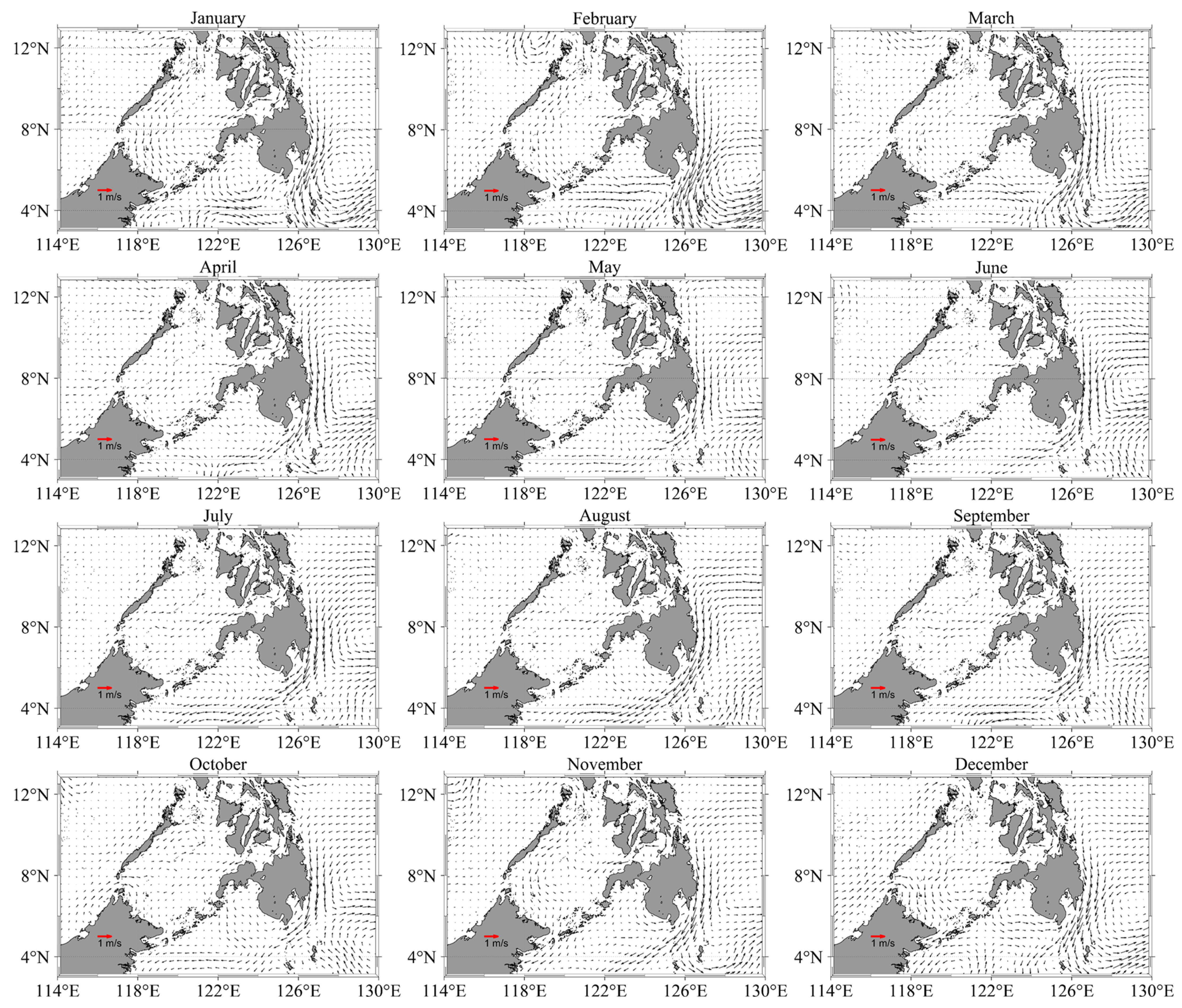
To depict the large-scale circulation in the Sulu Sea, we have used the geostrophic current derived from the satellite observed sea surface height, obtained from the E.U. Copernicus Marine Service. As shown in Figure 2, the typical circulation is characterized by a strong flow along the Palawan Island and the continental shelf on the western side of the Sulu Sea, forming a basin-scale loop during the winter and spring months. Part of the currents moves southward through the Sulu Archipelago into the Celebes Sea, while another part continues eastward along the Sulu Archipelago, forming a cyclonic circulation structure. This cyclonic structure is most prominent from January to February, while during other months, the circulation weakens and becomes less defined. Next, we systematically investigate the impact of the typical Sulu Sea circulation on ITs through a three-dimensional numerical simulation.
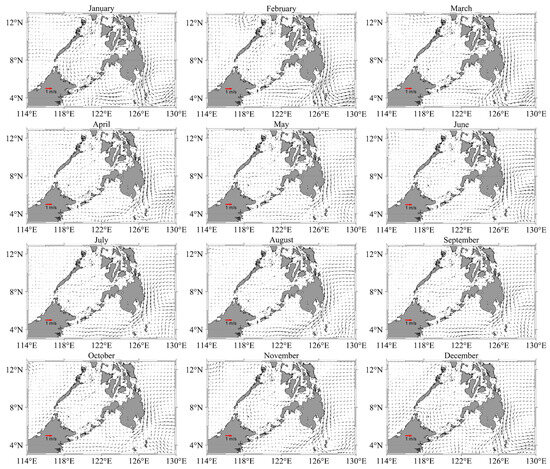
Figure 2.
Monthly mean sea surface circulation patterns in the Sulu Sea from January to December 2017, derived from satellite altimetry data.
2.2. Model Setup and Validation
To study the influence of circulation on the IT generation and propagation in the Sulu Sea, we first need to build an accurate circulation field in the Sulu Sea. To achieve this goal, we have employed the Massachusetts Institute of Technology general circulation model (MITgcm), which is widely used for simulating large-scale, mesoscale, and smaller-scale oceanic phenomena [32,33,34].
The simulation domain extends from 3° N to 27° N and 107° E to 130° E (Figure 1), encompassing the marginal seas adjacent to the Sulu Sea, including the South China Sea, the Philippine Sea, and the Celebes Sea. To ensure adequate resolution for both circulation and ITs, the horizontal resolution of the simulation is set to 1/24° × 1/24°, with a grid of 552 × 576 points. The vertical grid consists of 62 layers, with a uniform spacing of 10 m from the surface to 300 m depth. Below 300 m, layer spacing follows a hyperbolic tangent function, gradually increasing from 10 m at 300 m depth to 300 m near the seabed at 5000 m. The bathymetry data for the model are sourced from the General Bathymetric Chart of the Oceans (GEBCO) dataset, with a spatial resolution of 15 arc-second. The initial temperature, salinity fields, and open boundary forcing are derived from 5-day averaged Simple Ocean Data Assimilation (SODA) reanalysis data on 1 January 2014. The surface atmospheric forcing fields, including 2 m air temperature, 2 m specific humidity, 10 m wind components, and downward shortwave and longwave radiation fluxes, are sourced from 6-hourly National Centers for Environmental Prediction (NCEP) reanalysis data. The forcing fields are activated from the model start time, and the forcing intervals are interpolated to match the model’s time step. The model employs no-slip boundary conditions and hydrostatic assumption. Horizontal and vertical eddy viscosity coefficients are set to , while horizontal and vertical diffusion coefficients are set to . The time step is set to 100 s. To prevent baroclinic wave reflections at the boundaries, we set up 5 grids at the boundaries as a sponge layer.
The simulation is conducted in two steps. First, a 4-year circulation simulation from 1 January 2014 is performed under oceanic and atmospheric forcing. The initial temperature and salinity fields are set to be inhomogeneous, as derived from SODA data. After several years of integration, the circulation simulation reached a stable state. Second, tidal forcing, including the eight major tidal constituents (M2, S2, N2, K2, K1, O1, P1, and Q1) extracted from the Oregon State University TOPEX/Poseidon Global Inverse Solution tidal model (TPXO) data, is introduced at the model’s four boundaries on 16 November 2016, initiating a 130-day coupled circulation and IT simulation. Since the model requires approximately one month to reach stability, our analysis focuses on results from January to February 2017, when a typical cyclonic circulation pattern is observed by satellites in the Sulu Sea (Figure 2). This simulation is referred to as Case 1. A control experiment is conducted using the same grid and parameter settings, but it includes only tidal forcing at the boundaries, excluding surface atmospheric forcing and open boundary forcing for temperature, salinity, and currents, thus disregarding the circulation. To eliminate the influence of circulation, the initial temperature and salinity fields are set to be homogeneous, as derived from area-mean SODA data. This simulation is referred to as Case 2. The model configurations for the two cases are summarized in Table 1. By comparing the simulated results between Cases 1 and 2, we can effectively investigate the influence of circulation on IT generation and propagation in the Sulu Sea, providing valuable insights into the modulation of background circulation in modulating IT behaviors in marginal seas.

Table 1.
The setups of Case 1 and Case 2.
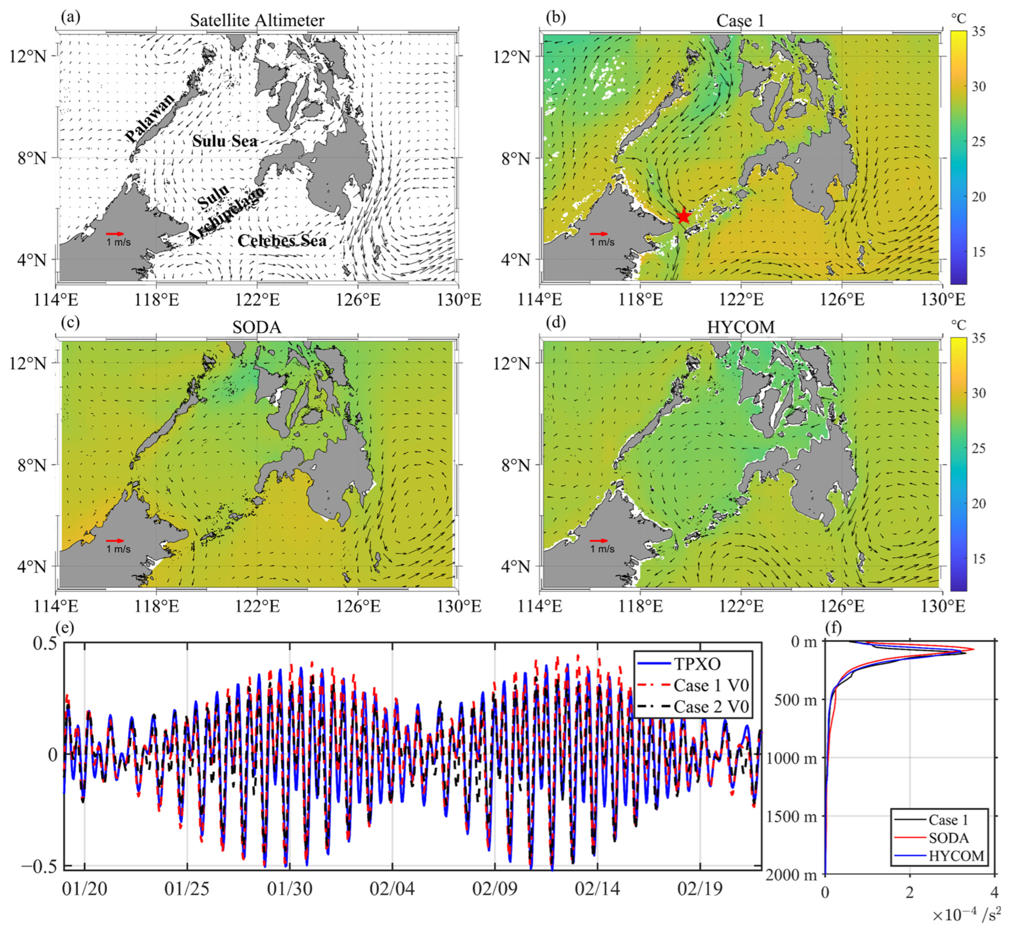
To validate the accuracy of the simulated circulation, the time-averaged velocity results from 20 January to 20 February 2017 are extracted from the circulation simulation and compared with the altimeter observations, as well as SODA and HYbrid Coordinate Ocean Model (HYCOM) reanalysis data. The cyclonic circulation structure in the Sulu Sea is consistently observed in satellite altimetry (Figure 3a), our model results (Figure 3b), and SODA (Figure 3c) and HYCOM data (Figure 3d). Additionally, the horizontal temperature distribution from the model generally matches that of SODA and HYCOM, demonstrating that the circulation model can effectively simulate the circulation and temperature characteristics of the Sulu Sea. For barotropic tide simulation, the simulated tidal currents are compared with the TPXO data at a position near the Sulu Archipelago (5.63° N, 119.67° E). The position is near the source region [9,10], which can effectively reflect the ITs’ generation condition (Figure 1). It is clear that the amplitude and phase of the simulated tidal currents closely align with those from the TPXO data (Figure 3e). Moreover, the area-mean stratification profile in the Sulu Sea from Case 1 is consistent with the results from SODA and HYCOM data (Figure 3f). These indicate that the model can accurately simulate the local barotropic tide and stratification characteristics, providing a reliable simulation of conditions in the ITs’ generation region.
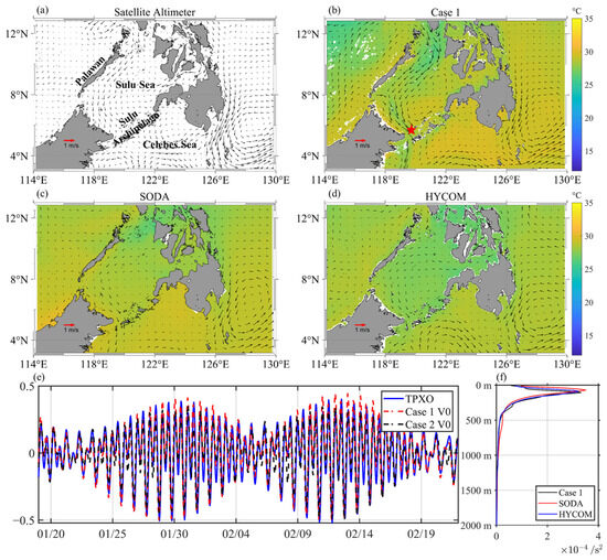
Figure 3.
(a–d) Mean sea surface temperature distributions and circulation patterns in the Sulu Sea from 20 January to 20 February 2017, derived from (a) satellite altimeter data, (b) Case 1, (c) SODA, and (d) HYCOM. (e) Comparison of barotropic tidal currents at the same location near the Sulu Archipelago (5.63° N, 119.67° E) between TPXO data and simulation results from Case 1 and Case 2. The red pentagram is the location of 5.63° N, 119.67° E. (f) Area-mean stratification profile in the Sulu Sea from Case 1, SODA, and HYCOM results, respectively.
2.3. Energy Diagnostic
To analyze the generation process of ITs, we adopt the tidally period-averaged depth-integrated baroclinic energy balance equation [35]:
where is the depth integration of a quantity from the bottom to the surface, and is the time average of a quantity over a period . is the bottom topography, and is the free surface elevation. The total water depth . This equation indicates that part of the baroclinic conversion is transformed into baroclinic energy flux , which radiates away from the generation sites, while the remaining portion is dissipated locally. Here, is baroclinic dissipation rate. The depth-integrated baroclinic energy flux () is given, respectively, by
where the velocity is divided into barotropic and baroclinic part as , where the barotropic velocity is defined as . The total density is expressed as , where is the constant reference density, is the background density, and is the perturbation density. The baroclinic perturbation pressure is given by . The barotropic-to-baroclinic energy conversion rate is given by [36,37]
where the vertical barotropic velocity is given by . is the vertical isopycnal displacement, and is the buoyancy frequency. The amplitude and phases of and at the major tidal frequency are represented by , , , and , respectively. We obtained the semi-diurnal and diurnal energy terms, specifically for the M2 and K1 tidal frequencies, through harmonic analysis.
Kang and Fringe (2012) [35] indicate that the dissipation is independent of viscosity and diffusion parameters in numerical simulations. Therefore, instead of computing the dissipation directly through viscosity and diffusion parameters, the dissipation term is obtained by Equation (1) based on the calculated conversion rate and energy flux.
2.4. Ray-Tracing Method
Besides the coupled circulation-IT model, we also used a theoretical framework, i.e., the tracing method, to further study the impact of circulation on IT propagation. The governing equations of the ray-tracing method are as follows [16]:
where and represent the horizontal coordinates, with denoting the east–west direction and representing the north–south direction. represents the arc length increment of the ray in the horizontal coordinate. and are the partial derivatives of the phase with respect to the horizontal coordinates, is the normalization factor, is the phase propagation direction, and represents the reciprocal of the IT phase speed along the direction . The Equations (4) and (5) are derived based on the definition of the arc length increment, , where represents the ray slope and is given by . The ray tracing is derived using Fermat’s Principle of Least Action and an eikonal equation based on the anisotropic background.
The IT phase speed is derived from the Taylor–Goldstein equation, which considers the effects of the background currents and the Coriolis parameter [22]:
where represents the vertical modal function, and is the horizontal wavenumber of ITs. The background currents and stratification are computed based on the model results. Detailed derivation of this ray-tracing method can refer to the work by Duda et al. (2018) [16].
3. Results
3.1. Modulation of Circulation on IT Generation
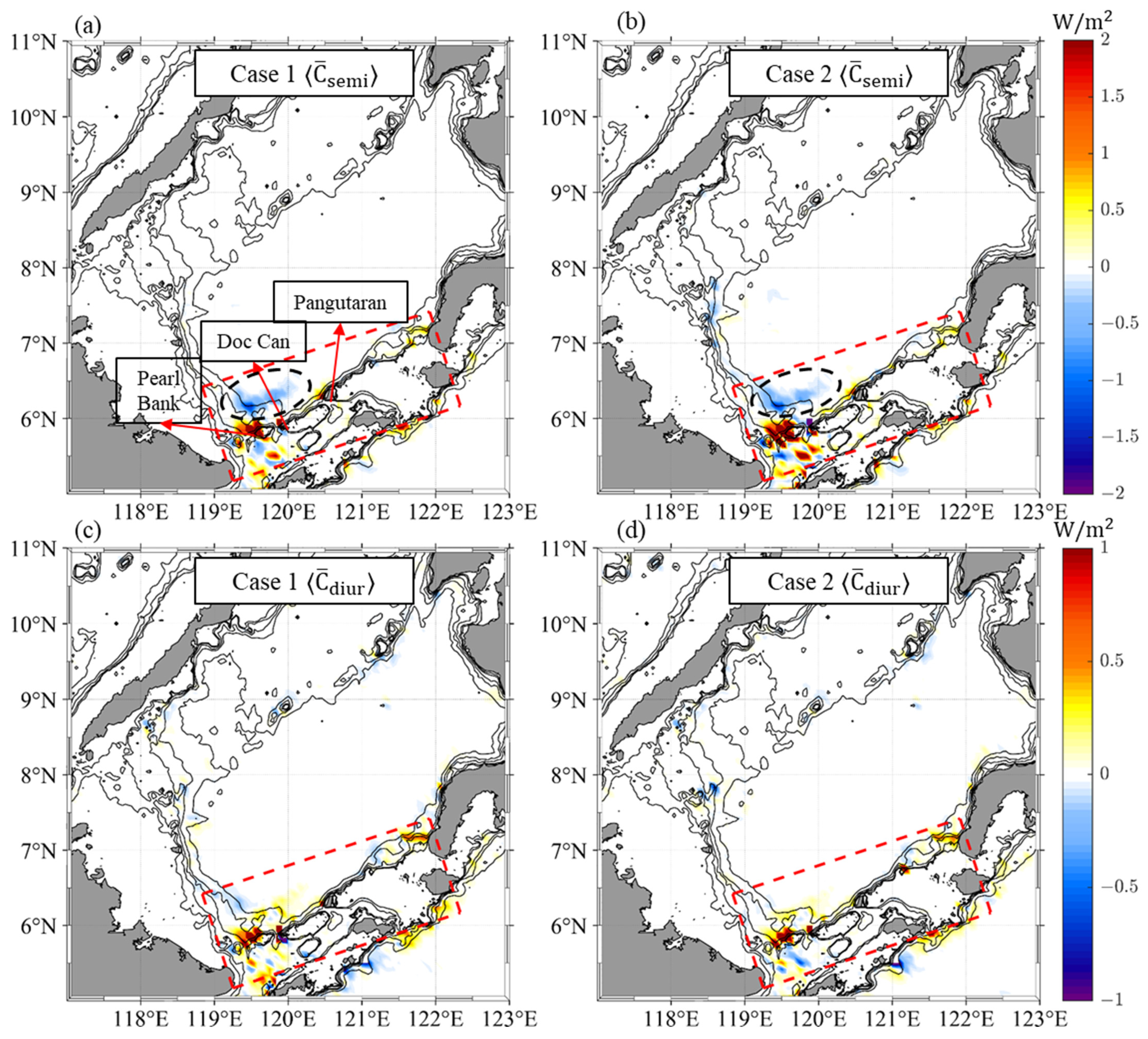
To evaluate the impact of the Sulu Sea circulation on IT generation, we calculated the depth-integrated and period-averaged baroclinic conversion rate using Equation (3) for both Cases 1 and 2 over the period from 20 January to 20 February 2017. The results are separated into semi-diurnal and diurnal components and are presented in Figure 4. As can be seen, the primary IT generation sites for both semi-diurnal and diurnal components are concentrated around the straits of the Sulu Archipelago, mainly in the regions around the Pearl Bank, Doc Can Island, and Pangutaran Island. To quantify IT generation, we integrated the baroclinic conversion rate at those main generation sites within the Sulu Archipelago (red dashed box in Figure 4). When there was no circulation (i.e., Case 2, Figure 4b,d), the calculated conversion rates for the semi-diurnal and diurnal ITs are 4.36 GW and 2.76 GW, respectively. In stark contrast, when circulation exists (i.e., Case 1, Figure 4a,c), the conversion rate of the semi-diurnal ITs reaches 5.12 GW, increasing by 17% compared to that in Case 2, and the conversion rate of diurnal ITs significantly increases by 77%, reaching as much as 4.88 GW. These comparisons highlight the significant role of Sulu Sea circulation in intensifying the interaction between barotropic tides and topography, particularly enhancing the generation of diurnal ITs.
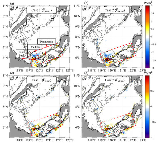
Figure 4.
Spatial distribution of the depth-integrated and period-averaged (a) semi-diurnal baroclinic conversion rate from Case 1, (b) semi-diurnal baroclinic conversion rate from Case 2, (c) diurnal baroclinic conversion rate from Case 1, and (d) diurnal baroclinic conversion rate from Case 2. Bathymetry is contoured at depths by thin black lines of −100, −200, −500, −1000, and −2000 m. The black dashed circles in (a,b) represent negative conversion zones.
Interestingly, the calculated results also demonstrate negative conversion zones for semi-diurnal ITs on the continental slope (black dashed circles in Figure 4a,b). This negative conversion reflects energy transfers from baroclinic back to barotropic forms, due to the phase difference between disturbances and local vertical barotropic currents , as suggested by previous studies [36,37]. The modulation of the circulation on IT phase speed may result in changes in the phase differences, thereby altering the magnitude of local negative conversion.
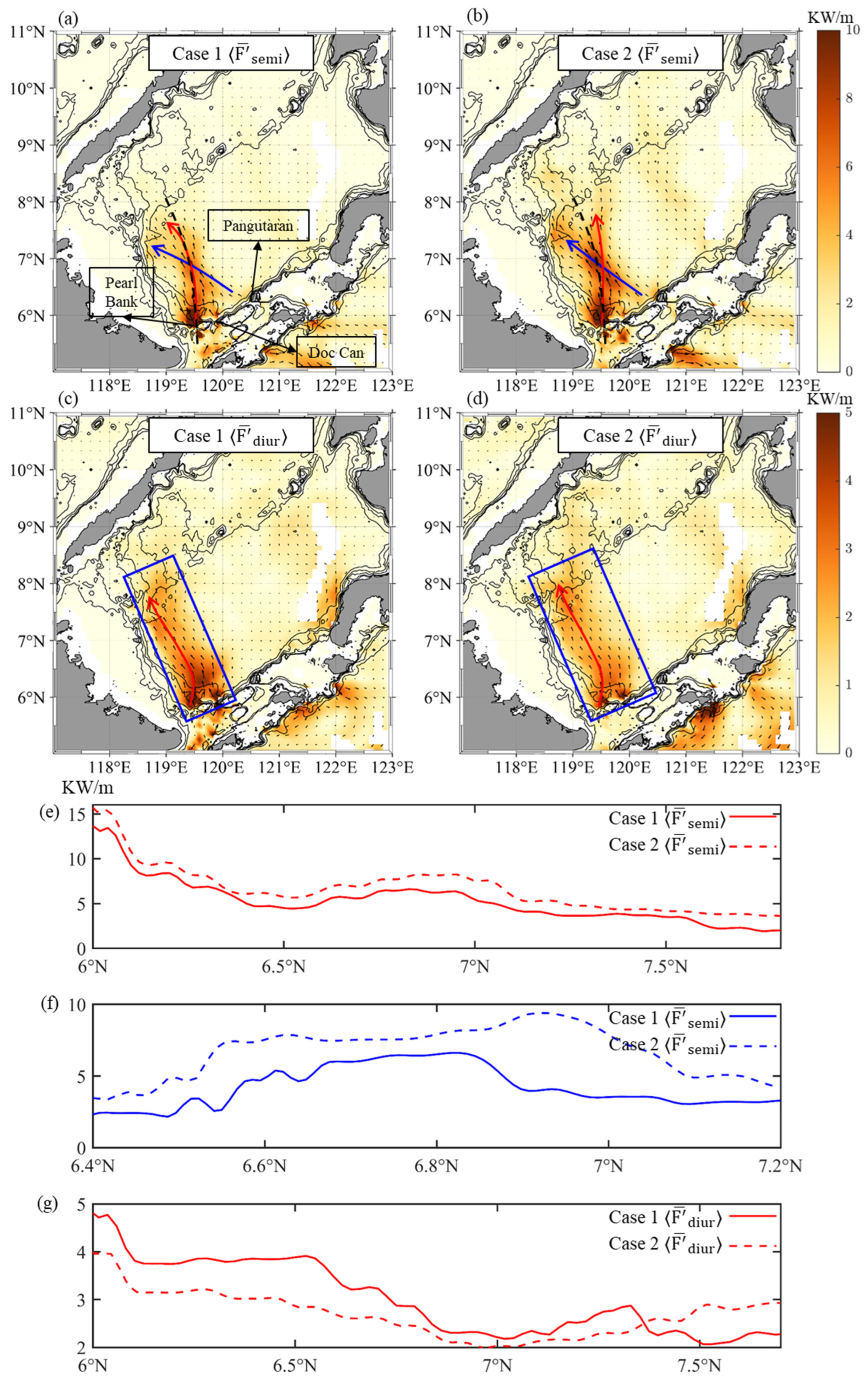
The horizontal distribution of the baroclinic energy flux provides further insights into IT generation patterns (Figure 5). In both Case 1 and Case 2, the semi-diurnal IT energy flux originating from the regions around Pearl Bank and Doc Can Island is more pronounced and propagates northward, while the flux from the region around Pangutaran Island is smaller and directed northwestward (Figure 5a,b). The convergence of these propagation routes enhances the local energy flux, with this effect being more noticeable in Case 2. The circulation influences the energy flux values from different source regions, thereby modulating the superposition of IT energy flux. For diurnal ITs, however, the primary sources are Pearl Bank and Doc Can Island, and no significant flux intersections are observed (Figure 5c,d).
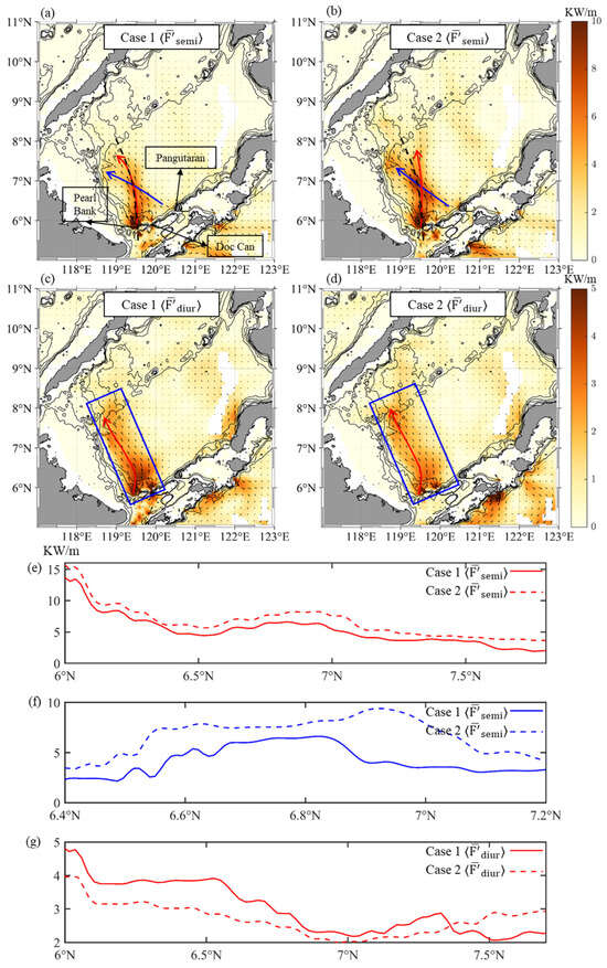
Figure 5.
Spatial distribution of the depth-integrated and period-averaged (a) semi-diurnal baroclinic energy flux from Case 1, (b) semi-diurnal baroclinic energy flux from Case 2, (c) diurnal baroclinic energy flux from Case 1, and (d) diurnal baroclinic energy flux from Case 2. Bathymetry is contoured at depths by thin black lines of −100, −200, −500, −1000, and −2000 m. Red arrows in (a,b) highlight the propagation routes of semi-diurnal ITs from source regions around Pearl Bank and Doc Can Island while blue arrows highlight the route of semi-diurnal ITs from the source region around Pangutaran Island. The black dashed line represents the selected transect for further analysis. Red arrows in (c,d) highlight the propagation routes of diurnal ITs from source regions around Pearl Bank and Doc Can Island. The blue boxes in (c,d) mark the flux cross-section. (e) The semi-diurnal energy flux along the red arrows in (a,b). (f) The semi-diurnal energy flux along the blue arrows in (a,b). (g) The diurnal energy flux along the red arrows in (c,d).
Although circulation enhances the generation of semi-diurnal ITs, the resulting energy flux in Case 1 is slightly weaker than in Case 2. Specifically, the average semi-diurnal energy flux along the red arrow in Figure 5a is 1.4 kW/m lower than that along the red arrow in Figure 5b (Figure 5e). Similarly, along the blue arrow in Figure 5a, the magnitude of the flux is reduced by an average of 2.5 kW/m compared to the blue arrow in Figure 5b (Figure 5f). These results indicate that the circulation plays a vital role in preventing the semi-diurnal energy from entering the Sulu Sea from its source region. Conversely, the circulation plays an opposite role in modulating the diurnal IT energy flux. It is observed that the diurnal IT energy flux in Case 1 increases by an average of 0.5 kW/m compared to Case 2 (Figure 5g), consistent with the variation rule of diurnal conversion rates under the influence of circulation.
The energy flux provides insight into the spatial distribution of (IT) energy, and energy flux divergence can reflect the overall magnitude of IT radiation from the source regions into the Sulu Sea. Analysis of baroclinic energy flux divergence around the generation regions reveals contrasting effects between the semi-diurnal and diurnal ITs. We have integrated the IT energy flux divergence around the source region. It is found that for semi-diurnal ITs, the integrated (in the same range with the red dashed box in Figure 4) energy flux divergence decreases by 41% in Case 1 (0.32 GW) compared to Case 2 (0.54 GW). In contrast, for diurnal ITs, flux divergence increases by 33%, rising from 0.27 GW in Case 2 to 0.36 GW in Case 1. This suggests that circulation can largely reduce/enhance the energy flux divergence of semi-diurnal/diurnal ITs. Additionally, we also obtained the baroclinic dissipation rates around source regions based on the baroclinic energy balance equation. Results show that in Case 2, the semi-diurnal and diurnal dissipation rates are −3.82 GW and −2.49 GW, respectively. However, when circulation comes to work, the semi-diurnal and diurnal dissipation rates increase to −4.80 GW and −4.52 GW in Case 1, respectively, showing the significant role of circulation in enhancing the baroclinic energy dissipation near the source regions.
The energy budget of the ITs in the Sulu Sea is summarized in Figure 6. We can find that while circulation enhances baroclinic conversion rates, it also raises dissipation proportions. When there is no circulation (Case 2), dissipation accounts for 88% and 90% of the conversion rates for semi-diurnal and diurnal ITs, respectively. If the circulation is included (Case 1), these proportions increase to 94% and 93%. Consequently, the proportion of baroclinic energy radiating away from the source regions decreases. For semi-diurnal ITs, this proportion declines from 12% to 6%, and for diurnal ITs, it decreases from 10% to 7%.
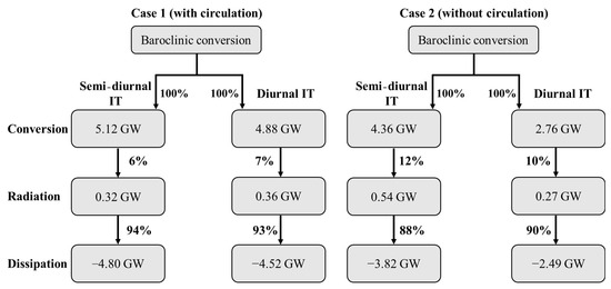
Figure 6.
Contribution of terms in energy budge from Case 1 and Case 2 results around the source region in the Sulu Archipelago (the red box in Figure 4).
3.2. Modulation of Circulation on IT Propagation
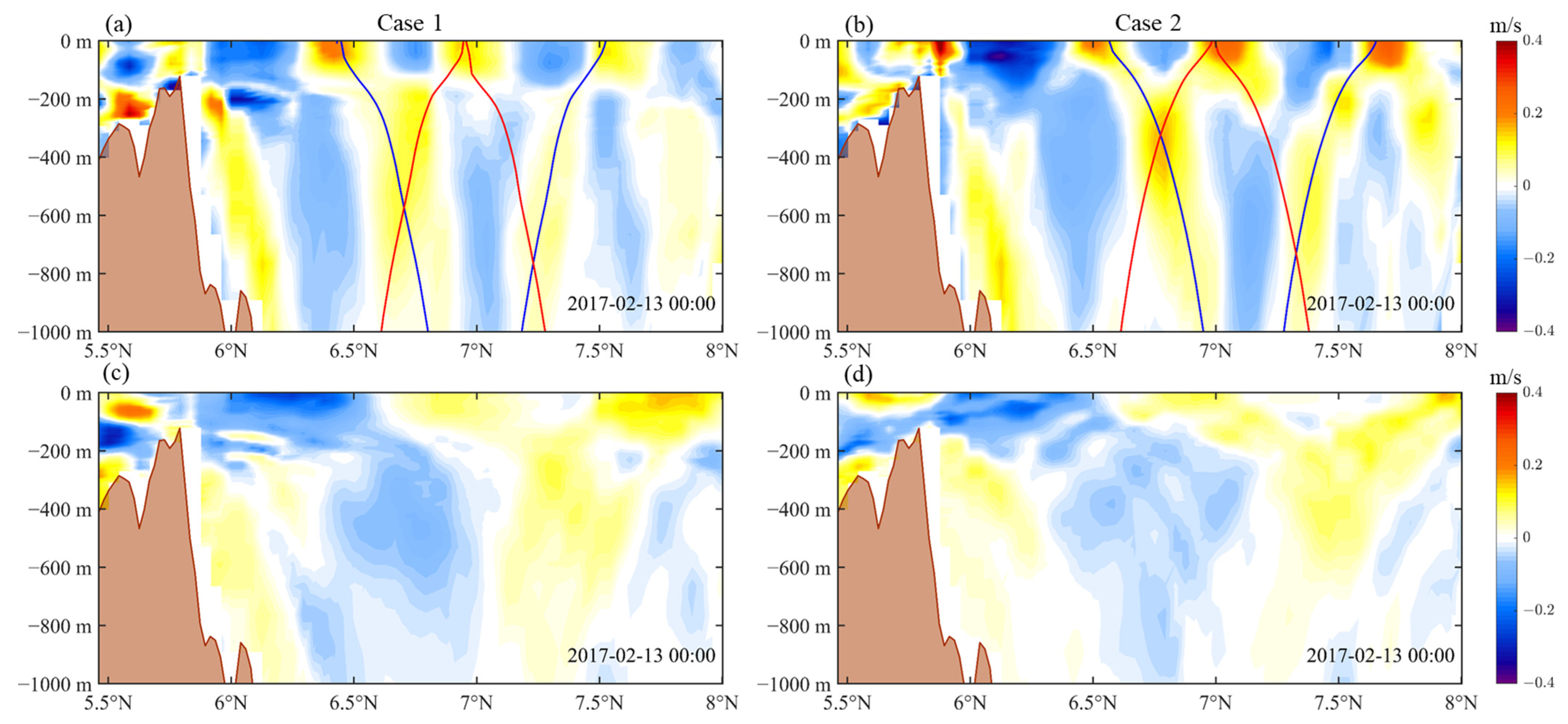
The circulation in the Sulu Sea not only influences IT generation but also modulates their propagation characteristics. To analyze the vertical structure of ITs during propagations, we selected a transect along the primary energy flux directions in both cases (indicated by dashed lines in Figure 5a,b) and extracted the meridional velocities along this transect (Figure 7). As shown in Figure 7a,c (i.e., Case 1), the maximum meridional velocity induced by semi-diurnal ITs is approximately 0.44 m/s, while diurnal ITs reach about 0.32 m/s. In comparison, the corresponding velocities in Case 2 (Figure 7b,d) are 0.48 m/s and 0.24 m/s, respectively. This comparison shows that circulation can reduce the velocity of semi-diurnal ITs but enhance that of diurnal ITs, a modulation rule that is consistent with that of energy flux as shown in Figure 5.
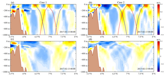
Figure 7.
Meridional velocity of (a) semi-diurnal ITs from Case 1, (b) semi-diurnal ITs from Case 2, (c) diurnal ITs from Case 1, and (d) diurnal ITs from Case 2 along the transect (the black dashed line in Figure 5) in the upper 1000 m. In subplots (a,b), the red and blue solid lines represent IT rays.
In Figure 7b, i.e., in the case of no circulation, we also presented the semi-diurnal IT rays that originated from the Pearl Bank and Doc Can Island regions (red solid lines) and the rays that originated from the Pangutaran Island region (blue solid lines). It is clear that these rays can intersect near 6.75° N, resulting in intensified IT energy, explaining the enhanced energy flux in the intersection region in Figure 5b. Similarly, when circulation is included (Figure 7a), similar ray intersections occur, but the resulting energy enhancement is weaker, consistent with the result in Figure 5a. For diurnal ITs (Figure 7c,d), there is no significant ray intersection within the transect due to the limited contribution from the Pangutaran Island region, which explains the relatively uniform energy flux distribution in Figure 5c,d.
The circulation in the Sulu Sea can significantly deflect IT pathways. When there is no circulation, the semi-diurnal IT energy fluxes radiated from the Pearl Bank and Doc Can Island region propagate mainly northward (red arrow in Figure 5b) and those radiated from the Pangutaran Island region propagate mainly northwestward (blue arrow in Figure 5b). In contrast, when circulation is included, northward fluxes from the Pearl Bank and Doc Can Island region are deflected westward (red arrow in Figure 5a), while northwestward fluxes from Pangutaran Island region are pushed further westward to the western slope at lower latitudes (blue arrow in Figure 5a). For diurnal ITs (Figure 5c,d), the circulation causes energy fluxes to converge westward, narrowing the flux cross-section and increasing flux intensity along their propagation path.
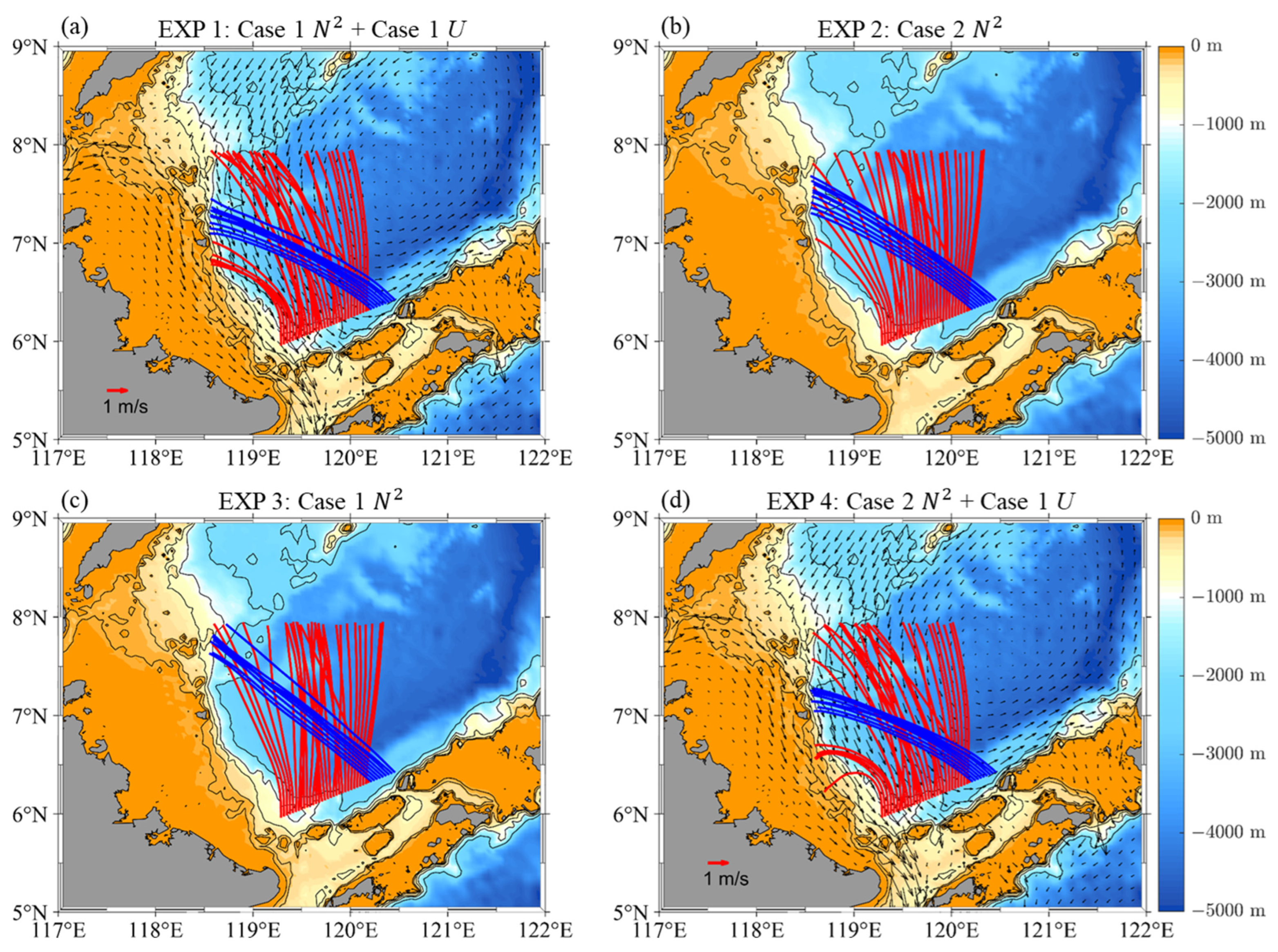
To investigate the mechanisms behind semi-diurnal IT refraction, the ray-tracing method (Equations (4)–(10)) was applied using the simulated temperature, salinity, and current fields (Table 2). Initial ray positions were selected near the three main IT source regions, with initial directions aligned to the mean energy flux directions (Figure 5a,b). The ray-tracing results for M2 ITs using the simulated fields in Case 1 (EXP 1) and Case 2 (EXP 2) are shown in Figure 8a,b, respectively. When there is no circulation (Figure 8b), the IT rays show an evident westward deflection, due to the east–west bathymetric gradient in the Sulu Sea. This westward deflection can be further intensified by the cyclonic circulation (Figure 8a), which emerges in the circulation-couple simulation. The propagation direction variations predicted by the ray-tracing method closely match the semi-diurnal IT energy flux patterns (red and blue arrows in Figure 5a,b).
Table 2.
Comparison of parameter setups for the ray-tracing method.
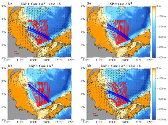
Figure 8.
The results of the ray-tracing method for M2 ITs in the same time under different conditions (the red lines represent the IT rays from source regions around Pearl Bank and Doc Can Island, while the blue lines represent the IT rays from the source region around Pangutaran Island): (a) background currents and stratification from Case 1, (b) stratification from Case 2 and no background currents, (c) stratification from Case 1 and no background currents, and (d) stratification from Case 2 and background currents from Case 1. Bathymetry is contoured at depths by thin black lines of −100, −200, −500, −1000, and −2000 m.
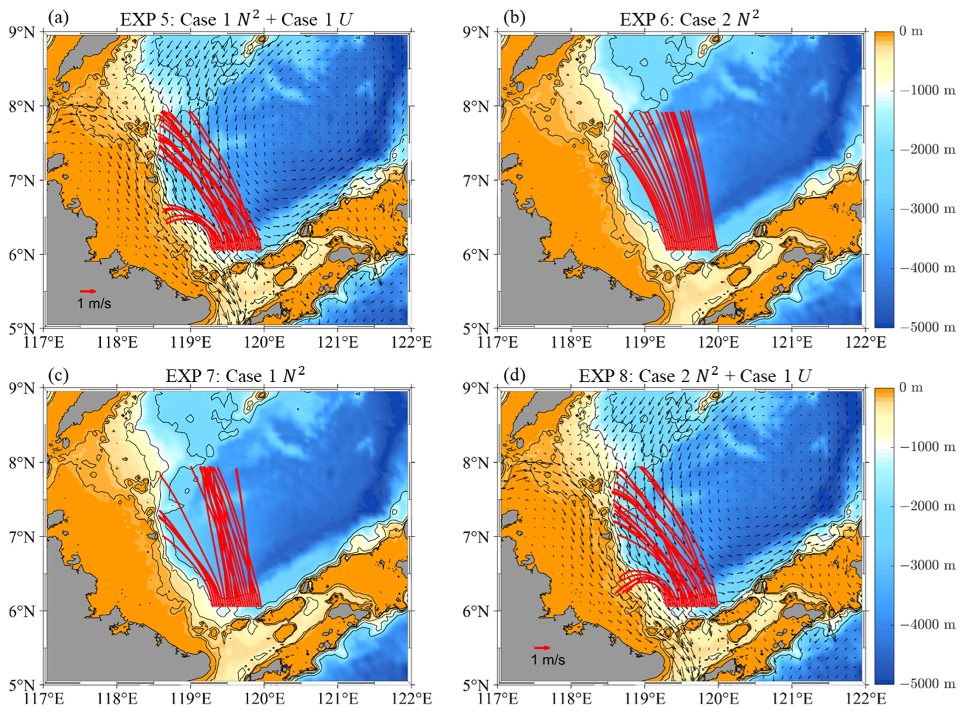
To further clarify the roles of the background currents and stratification induced by the circulation in IT refraction, two sensitivity experiments were conducted: (1) using the stratification from Case 1 without background currents (EXP 3); (2) using the stratification from Case 2 combined with the background currents from Case 1 (EXP 4). The corresponding ray-tracing results are shown in Figure 8c,d, respectively. By comparing the results between EXP2 (Figure 8b) and EXP 3 (Figure 8c), we can find that the horizontal variations in stratification have a minor impact on IT ray directions. In contrast, when comparing the results between EXP2 (Figure 8b) and EXP 4 (Figure 8d), the horizontal background currents are found to play an important role in determining IT ray refraction. Background currents predominantly drive the westward refraction of IT rays, while stratification slightly suppresses this refraction. Similarly, the ray-tracing results for K1 ITs using the simulated fields (EXP 5–8 in Table 2) are shown in Figure 9. The Sulu circulation modulates the westward refraction of K1 IT rays, narrowing their cross-section. This behavior is consistent with the diurnal IT energy flux patterns shown in Figure 5c,d. The effects of background currents and stratification on K1 IT rays are similar to M2 IT rays.
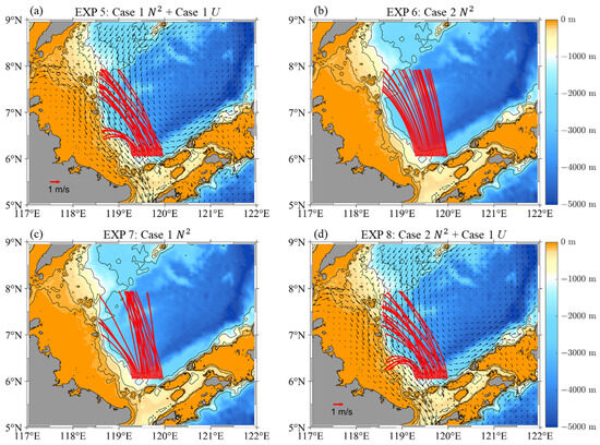
Figure 9.
The results of the ray-tracing method for K1 ITs in the same time under different conditions (the red lines represent the IT rays from source regions around Pearl Bank and Doc Can Island): (a) background currents and stratification from Case 1, (b) stratification from Case 2 and no background currents, (c) stratification from Case 1 and no background currents, and (d) stratification from Case 2 and background currents from Case 1. Bathymetry is contoured at depths by thin black lines of −100, −200, −500, −1000, and −2000 m.
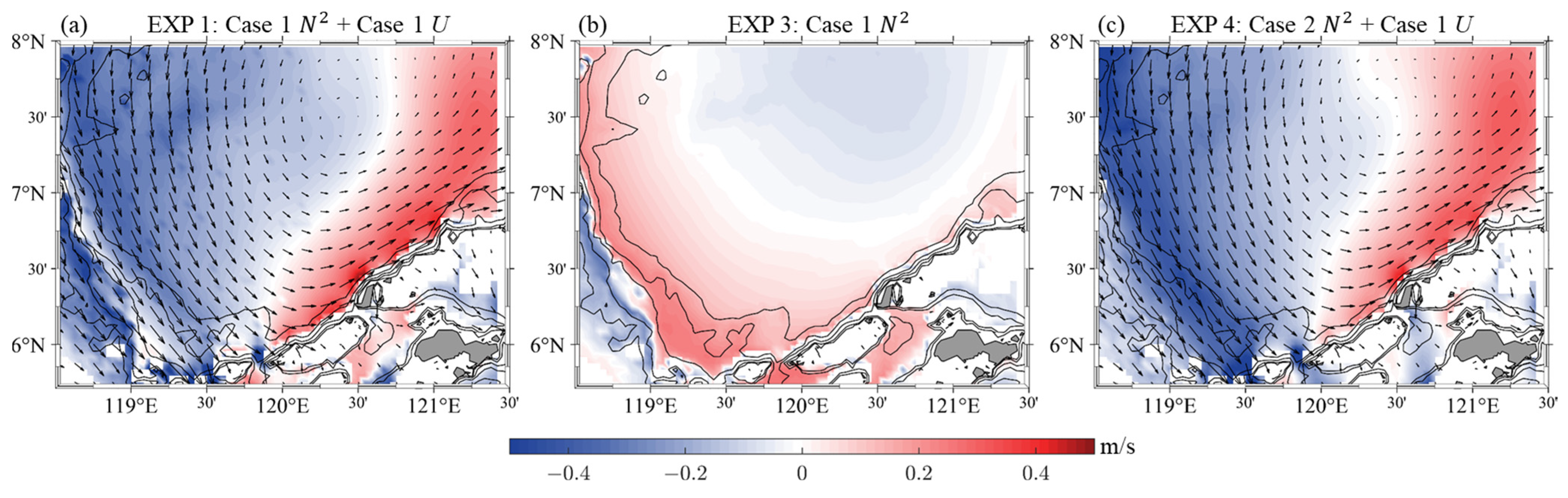
It is known that the refraction of IT rays is directly determined by the distribution of propagation speeds in the propagation path. We have further calculated the IT propagation speeds corresponding to the four cases in Figure 8, using Equation (10). To remove the influence of topographic gradients on propagation speeds, the propagation speeds for EXP 1, EXP 3, and EXP 4 in Figure 8a,c,d relative to the propagation speeds for EXP 2 in Figure 8b are calculated, and the results of propagation speed differences are shown in Figure 10.

Figure 10.
Using the theoretical phase speed calculated from Case 2 results as a reference, the variations in phase speed from Case 1 modulated by (a) both the background stratification and background currents, (b) only the background stratification, and (c) only the background currents. Bathymetry is contoured at depths by thin black lines of −100, −200, −500, −1000, and −2000 m.
When considering only the effect of the background currents (Figure 10c), the cyclonic circulation forms two distinct regions: a southward current region near the western slope and a northeastward current region near the eastern Sulu Archipelago. In the southward current region, IT propagation is slowed by up to −0.4 m/s, while in the northeastward current region, propagation is accelerated by up to 0.3 m/s. This west-to-east gradient of decreasing-to-increasing speed drives pronounced westward deflection of IT rays.
Stratification-induced modulation of propagation speeds exhibits a different spatial pattern (Figure 10b), with deceleration in the basin center and acceleration at the edges. This pattern reflects well the modulation of circulation on the thermocline variation, i.e., deepening the thermocline at the edges while elevating it in the center, as a deeper/shallower thermocline can lead to faster/slower propagation speeds [38]. As a result, IT rays converge toward the basin center. When both background currents and stratification are considered (Figure 10a), the modulation by background currents dominates. The overall spatial characteristic of the propagation speeds closely resembles that in Figure 10c. These analyses highlight the significant role of circulation-induced background current in modulating the horizontal distribution of propagation speeds of ITs and ultimately determining the IT ray refraction.
Therefore, the influence of the Sulu Sea cyclonic circulation on IT propagation can be categorized into two mechanisms. The first is the Doppler effect induced by background currents, which is particularly prominent in strong current regions such as the Gulf Stream (Duda et al., 2018) [16] and the Kuroshio (Xu et al., 2021) [18], where background currents alter IT propagation paths. The second mechanism is the suppression of westward IT refraction due to the stratification induced by the Sulu Sea cyclonic circulation, which is analogous to the influence of mesoscale eddies. As observed by Huang et al. (2018) [22] in the Luzon Strait, anticyclonic eddies induce clockwise IT refraction, whereas cyclonic eddies result in counterclockwise refraction.
4. Discussion
Xu et al. (2021) [18] have shown that generation and energy flux enhancement of semi-diurnal and diurnal ITs in the Luzon Strait, influenced by the Kuroshio, are consistent while the effects of circulation on the two types of ITs exhibit significant differences in the Sulu Sea. To better understand the influence of circulation on the generation rates of semi-diurnal and diurnal ITs, we calculated the positive and negative baroclinic energy conversion rates for both Case 1 (with circulation) and Case 2 (without circulation). The results show that in Case 1, the positive conversion rate for semi-diurnal ITs is 7.31 GW, while the negative rate is −2.20 GW. In Case 2, the positive rate increases to 9.37 GW, and the negative rate is −5.01 GW. For diurnal ITs, Case 1 exhibits a positive conversion rate of 6.02 GW and a negative rate of −1.14 GW, while in Case 2, these values are 3.53 GW and −0.77 GW, respectively. The positive and negative terms in conversion rates for the two cases are summarized in Table 3.
Table 3.
Contribution of positive and negative terms in conversion rates from Case 1 and Case 2 results around the source region in the Sulu Archipelago (the red box in Figure 4).
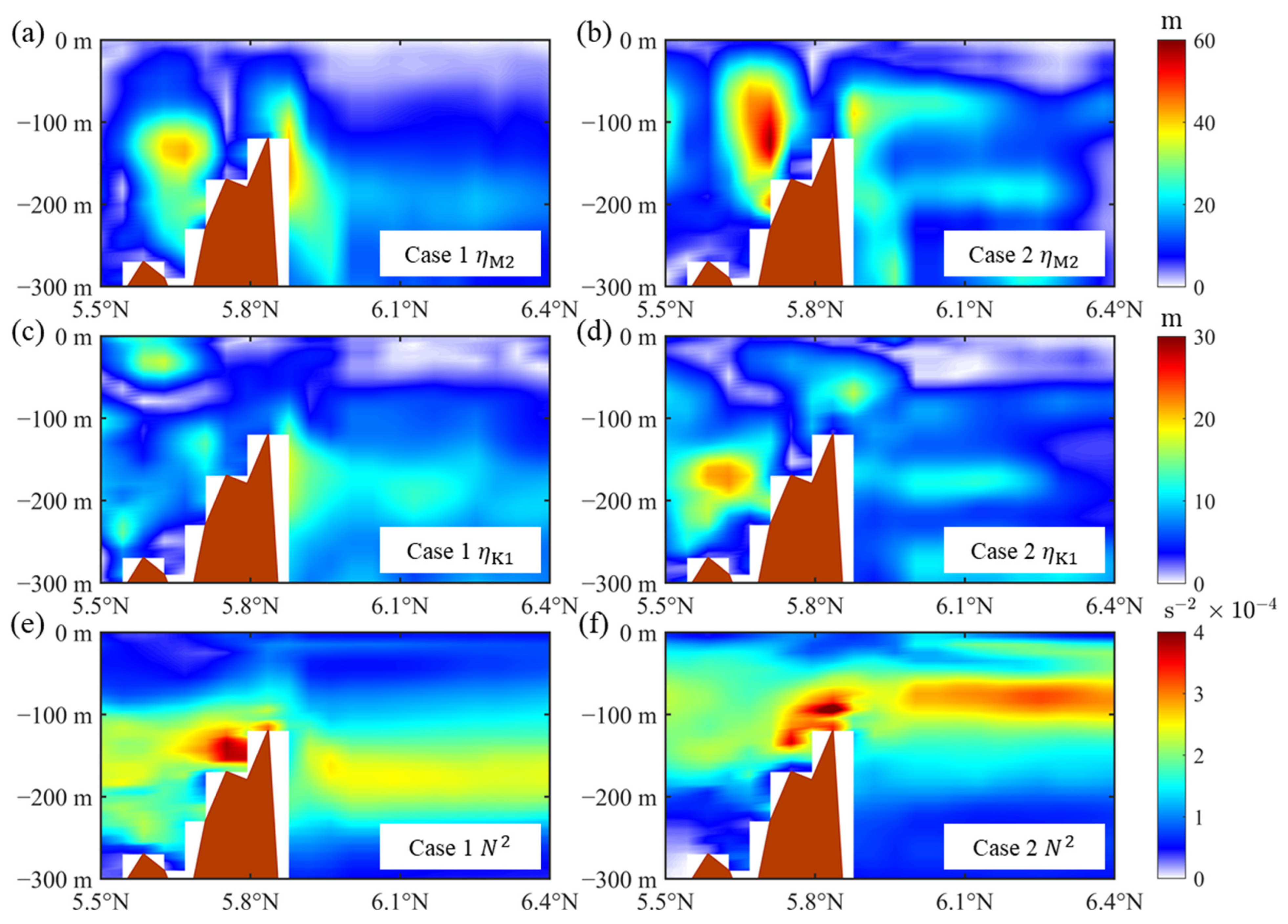
To investigate the mechanisms behind these differences, we examined the contributions of each term in the energy conversion equation (Equation (3)) along the transect indicated by the black dashed lines in Figure 5. For the semi-diurnal IT (M2), in the absence of circulation (Case 2), the around the submarine ridge is mainly concentrated between 30 m and 200 m (Figure 11b), roughly aligning with the concentration range of (Figure 11f). When circulation is included (Case 1), this range shifts downward to 90–250 m (Figure 11a), along with a similar shift in (Figure 11e). Additionally, circulation reduces the magnitude of , leading to a smaller integral around the source region in Case 1 compared to Case 2, which is clearly shown in Figure 12a.
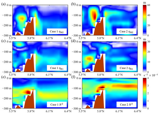
Figure 11.
(a) Amplitude of the vertical isopycnal displacement for M2 ITs, (c) amplitude of the vertical isopycnal displacement for K1 ITs, and (e) buoyancy frequency in Case 1 along the transect as shown in Figure 7. Panels (b,d,f) are the same as (a,c,e) but in Case 2.
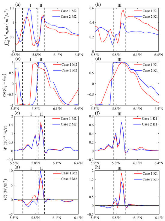
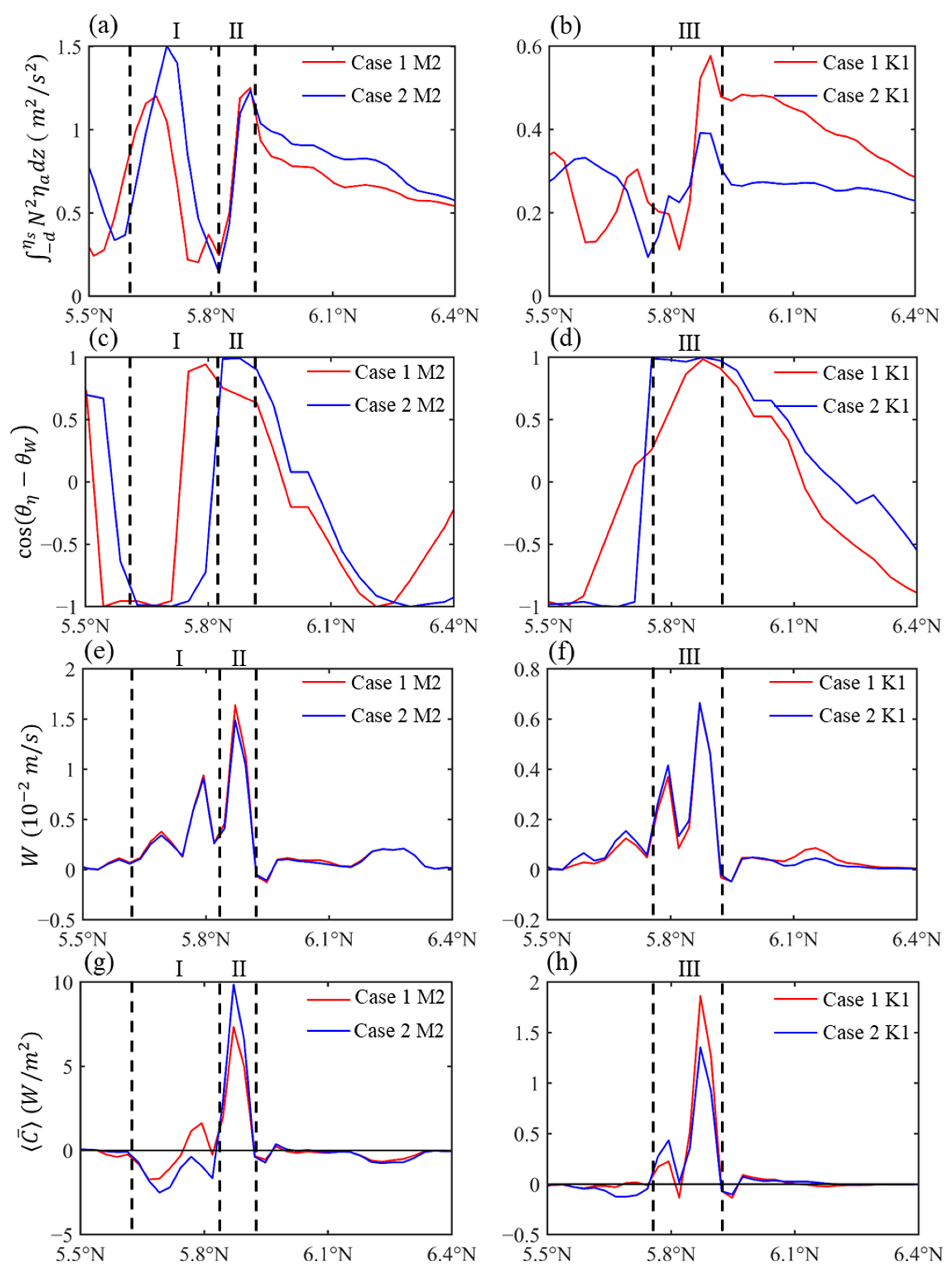
Figure 12.
The (a) integral , (c) , (e) amplitude of vertical barotropic velocity , and (g) generation rate for the M2 frequency along the transect as shown in Figure 7. The red and blue curves represent Case 1 and Case 2, respectively. Panels (b,d,f,h) are the same as (a,c,e,g) but for the K1 frequency.
Further analysis of the barotropic tidal currents between Case 1 and Case 2 (Figure 3e) shows that the magnitude and phase of these currents remain largely unchanged by the circulation. This suggests that the vertical barotropic velocity () and its phase () are little affected by circulation, as confirmed by Figure 12e. However, circulation alters the phase of () by modifying the propagation speed of disturbances, which in turn affects the value of (Figure 12c). The variation in the conversion rate is the combined effects of the changes in and . It is found that the positive conversion in Case 1 is lower than in Case 2 (range II in Figure 12g), which is primarily due to differences in between Case 1 and Case 2 (range II in Figure 12c). The negative conversion in Case 1 is also lower than in Case 2 (range I in Figure 12g), which can be attributed to the larger in Case 2 (range I in Figure 12a). Therefore, it is the difference in the or between Case 1 and Case 2 that explains why the positive semi-diurnal generation rate in Case 1 (7.31 GW) is lower than that in Case 2 (9.37 GW), and the negative semi-diurnal generation rate in Case 1 (−2.20 GW) is smaller than that in Case 2 (−5.01 GW).
For the diurnal IT (K1), in the absence of circulation, the around the submarine ridge is mainly concentrated between 100 m and 250 m (Figure 11d), while the is mainly concentrated tween 30 m and 180 m, with its peak locating at about 80 m (Figure 11f). When circulation is present, the around the submarine ridge also concentrates approximately between 100 m and 240 m (Figure 11c), but the concentration range of shifts downward (Figure 11e), roughly aligning with the concentration range of the . Although the magnitude of is slightly reduced with circulation, the closer alignment of with in Case 1 results in a larger compared to Case 2 (Figure 12b). Additionally, the corresponding is also influenced by the circulation (Figure 12d). It is found that the positive conversion in Case 1 is evidently larger than in Case 2 (range III in Figure 12h), mainly resulting from the larger (range III in Figure 12b). The negative conversions in Case 1 and Case 2 are both small and nearly identical. These results can explain why the positive diurnal generation rate in Case 1 (6.02 GW) is larger than in Case 2 (3.53 GW), and the negative diurnal generation rate in Case 1 (−1.14 GW) is similar with in Case 2 (−0.77 GW).
As can been seen, by modulating the or , the circulation can enhance the conversion rate of diurnal ITs but reduce the conversion rate of semi-diurnal ITs. However, the influence on the variations of positive and negative conversion rates is different. For diurnal ITs, circulation significantly enhances the positive conversion rate, while the variation in negative conversion rate is minimal. In contrast, the semi-diurnal ITs show a large reduction in conversion when circulation is present, and the reduction in the negative conversion rate is even larger than the positive conversion rate. As a result, both the diurnal and semi-diurnal ITs demonstrate an increase in the net energy conversion rate, but the increased portion of diurnal ITs is more significant than the semi-diurnal ITs, as summarized in Figure 6.
5. Conclusions
This study for the first time investigates the influence of the Sulu Sea circulation on IT generation and propagation using three-dimensional numerical simulation results. The comparison of energy diagnostics and budgets with and without circulation in the Sulu Archipelago IT source regions reveal that Sulu Sea circulation significantly enhances the conversion rates. Specifically, the conversion of semi-diurnal IT increases by approximately 17%, while that of diurnal IT rises by about 77%. This different rate of increase between semi-diurnal and diurnal ITs is due to the different influences of circulation on the positive and negative conversion rates for semi-diurnal and diurnal ITs, determined by the patterns of vertical isopycnal displacement and buoyancy frequency, as well as the phase lag between displacements and vertical barotropic velocity. Furthermore, the circulation markedly intensifies the dissipation of IT energy near the source regions, causing a larger proportion of conversion energy to be dissipated locally. Consequently, the proportion of IT energy flux radiating into the Sulu Sea basin relative to conversion decreases. Overall, the circulation reduces the radiated energy flux of semi-diurnal ITs but enhances that of diurnal ITs.
Analysis of the IT transect structure and ray-tracing results shows that the cyclonic circulation within the Sulu Sea basin significantly affects IT propagation speeds. In the counter-current region, the phase speed of ITs decreases while the phase speed of ITs increases in the co-current region. The spatially inhomogeneous propagation speeds result in pronounced westward refraction of IT rays during horizontal propagation. Sensitivity experiments about the effects of the background currents and stratification induced by the circulation indicate that the stratification weakens the westward refraction of IT rays, while the background currents strengthen the westward refraction. Among these, the influence of the background currents field is dominant.
This study reveals the modulation effect of the southward circulation in the Sulu Sea on IT generation and propagation through analysis of model results. Although the annual mean circulation in the Sulu Sea predominantly exhibits a southward cyclonic pattern, its intensity, direction, and structure exhibit significant seasonal variations. These temporal changes in circulation add complexity to its modulation on ITs, warranting further analysis and research on these dynamic processes in future studies.
Author Contributions
Conceptualization, X.H., Y.R. and H.L.; methodology, X.H., Y.R. and H.L.; software, Y.R., H.L. and J.L.; validation, Y.R. and H.L.; formal analysis, Y.R.; investigation, Y.R. and H.L.; resources, X.H.; data curation, Y.R. and H.L.; writing—original draft preparation, Y.R.; writing—review and editing, C.W., Y.Y. and H.L.; visualization, Y.R.; supervision, Y.Y.; project administration, X.H.; funding acquisition, X.H. All authors have read and agreed to the published version of the manuscript.
Funding
This study was supported by the National Key R&D Program of China (Grant 2023YFC3106400), Hainan Provincial NanHaiXinXing Project (Grant NHXXRCXM202364), Hainan Province Science and Technology Fund (Grant SOLZSKY2025005), National Natural Science Foundation of China (Grants 92258301 and 42406016) and Hainan Province Science and Technology Special Fund (Grants ZDYF2023GXJS151 and ZDYF2023GXJS149).
Data Availability Statement
The model data presented in this study are available on request from the corresponding author.
Acknowledgments
We acknowledge the use of the MIOST-IT (The Multivariate Inversion of Ocean Surface Topography-Internal Tide Model) dataset from AVISO (https://www.aviso.altimetry.fr), accessed on 28 July 2023. The satellite altimeter products are from the EU Copernicus Ocean State Report (https://data.marine.copernicus.eu/product/SEALEVEL_GLO_PHY_L4_MY_008_047), accessed on 18 October 2024. The surface atmospheric forcing data are downloaded from the NCEP (National Centers for Environmental Prediction) Reanalysis 1 project (https://psl.noaa.gov/data/gridded/data.ncep.reanalysis.html), accessed on 23 September 2024. The bathymetric dataset is downloaded from GEBCO (The General Bathymetric Chart of the Oceans) data (https://www.gebco.net/), accessed on 16 November 2022. The barotropic tide amplitudes and phase are derived from TPXO (the Oregon State University TOPEX/Poseidon Global Inverse Solution tidal model) data (https://www.tpxo.net/), accessed on 29 September 2021. The SODA (Simple Ocean Data Assimilation) product is available at https://soda.umd.edu/, accessed on 19 October 2024. The HYCOM (HYbrid Coordinate Ocean Model) product is available at https://www.hycom.org/, accessed on 19 October 2024. The MITgcm (Massachusetts Institute of Technology general circulation model) used for simulations is available at https://mitgcm.org/source-code/.
Conflicts of Interest
The authors declare no conflicts of interest.
References
- Alford, M.H. Redistribution of energy available for ocean mixing by long-range propagation of internal waves. Nature 2003, 423, 159–162. [Google Scholar] [CrossRef]
- Zhao, Z.; Alford, M.H.; Girton, J.B.; Rainville, L.; Simmons, H.L. Global Observations of Open-Ocean Mode-1 M2 Internal Tides. J. Phys. Oceanogr. 2016, 46, 1657–1684. [Google Scholar] [CrossRef]
- Rudnick, D.L.; Boyd, T.J.; Brainard, R.E.; Carter, G.S.; Egbert, G.D.; Gregg, M.C.; Holloway, P.E.; Klymak, J.M.; Kunze, E.; Lee, C.M.; et al. From Tides to Mixing Along the Hawaiian Ridge. Science 2003, 301, 355–357. [Google Scholar] [CrossRef] [PubMed]
- Floor, J.W.; Auclair, F.; Marsaleix, P. Energy transfers in internal tide generation, propagation and dissipation in the deep ocean. Ocean Model. 2011, 38, 22–40. [Google Scholar] [CrossRef]
- Munk, W.; Wunsch, C. Abyssal recipes II: Energetics of tidal and wind mixing. Deep Sea Res. Part I Oceanogr. Res. Pap. 1998, 45, 1977–2010. [Google Scholar] [CrossRef]
- Wunsch, C.; Ferrari, R. Vertical Mixing, Energy, and the General Circulation of the Oceans. Annu. Rev. Fluid Mech. 2004, 36, 281–314. [Google Scholar] [CrossRef]
- Apel, J.R.; Holbrook, J.R.; Liu, A.K.; Tsai, J.J. The Sulu Sea Internal Soliton Experiment. J. Phys. Oceanogr. 1985, 15, 1625–1651. [Google Scholar] [CrossRef]
- Liu, B.; D’Sa, E.J. Oceanic Internal Waves in the Sulu–Celebes Sea Under Sunglint and Moonglint. IEEE Trans. Geosci. Remote Sens. 2019, 57, 6119–6129. [Google Scholar] [CrossRef]
- Nagai, T.; Hibiya, T. Internal tides and associated vertical mixing in the Indonesian Archipelago. J. Geophys. Res. Ocean. 2015, 120, 3373–3390. [Google Scholar] [CrossRef]
- Zhao, X.; Xu, Z.; Feng, M.; Li, Q.; Zhang, P.; You, J.; Gao, S.; Yin, B. Satellite Investigation of Semidiurnal Internal Tides in the Sulu-Sulawesi Seas. Remote Sens. 2021, 13, 2530. [Google Scholar] [CrossRef]
- Rainville, L.; Pinkel, R. Propagation of Low-Mode Internal Waves through the Ocean. J. Phys. Oceanogr. 2006, 36, 1220–1236. [Google Scholar] [CrossRef]
- Ponte, A.L.; Klein, P. Incoherent signature of internal tides on sea level in idealized numerical simulations. Geophys. Res. Lett. 2015, 42, 1520–1526. [Google Scholar] [CrossRef]
- Masunaga, E.; Uchiyama, Y.; Suzue, Y.; Yamazaki, H. Dynamics of Internal Tides Over a Shallow Ridge Investigated with a High-Resolution Downscaling Regional Ocean Model. Geophys. Res. Lett. 2018, 45, 3550–3558. [Google Scholar] [CrossRef]
- Rainville, L.; Lee, C.M.; Rudnick, D.L.; Yang, K. Propagation of internal tides generated near Luzon Strait: Observations from autonomous gliders. J. Geophys. Res. Ocean. 2013, 118, 4125–4138. [Google Scholar] [CrossRef]
- Alford, M.H.; Peacock, T.; MacKinnon, J.A.; Nash, J.D.; Buijsman, M.C.; Centurioni, L.R.; Chao, S.; Chang, M.; Farmer, D.M.; Fringer, O.B.; et al. The formation and fate of internal waves in the South China Sea. Nature 2015, 521, 65–69. [Google Scholar] [CrossRef]
- Duda, T.F.; Lin, Y.; Buijsman, M.; Newhall, A.E. Internal Tidal Modal Ray Refraction and Energy Ducting in Baroclinic Gulf Stream Currents. J. Phys. Oceanogr. 2018, 48, 1969–1993. [Google Scholar] [CrossRef]
- Masunaga, E.; Uchiyama, Y.; Yamazaki, H. Strong Internal Waves Generated by the Interaction of the Kuroshio and Tides over a Shallow Ridge. J. Phys. Oceanogr. 2019, 49, 2917–2934. [Google Scholar] [CrossRef]
- Xu, Z.; Wang, Y.; Liu, Z.; McWilliams, J.C.; Gan, J. Insight Into the Dynamics of the Radiating Internal Tide Associated With the Kuroshio Current. J. Geophys. Res. Ocean. 2021, 126, e2020JC017018. [Google Scholar] [CrossRef]
- Tang, G.; Deng, Z.; Chen, R.; Xiu, F. Effects of the Kuroshio on internal tides in the Luzon Strait: A model study. Front. Mar. Sci. 2023, 9, 995601. [Google Scholar] [CrossRef]
- Park, J.; Watts, D.R. Internal Tides in the Southwestern Japan/East Sea. J. Phys. Oceanogr. 2006, 36, 22–34. [Google Scholar] [CrossRef]
- Kerry, C.G.; Powell, B.S.; Carter, G.S. The Impact of Subtidal Circulation on Internal Tide Generation and Propagation in the Philippine Sea. J. Phys. Oceanogr. 2014, 44, 1386–1405. [Google Scholar] [CrossRef]
- Huang, X.; Wang, Z.; Zhang, Z.; Yang, Y.; Zhou, C.; Yang, Q.; Zhao, W.; Tian, J. Role of Mesoscale Eddies in Modulating the Semidiurnal Internal Tide: Observation Results in the Northern South China Sea. J. Phys. Oceanogr. 2018, 48, 1749–1770. [Google Scholar] [CrossRef]
- Cai, T.; Zhao, Z.; D’Asaro, E.; Wang, J.; Fu, L. Internal Tide Variability Off Central California: Multiple Sources, Seasonality, and Eddying Background. J. Geophys. Res. Ocean. 2024, 129, e2024JC020892. [Google Scholar] [CrossRef]
- Fan, L.; Sun, H.; Yang, Q.; Li, J. Numerical investigation of interaction between anticyclonic eddy and semidiurnal internal tide in the northeastern South China Sea. Ocean Sci. 2024, 20, 241–264. [Google Scholar] [CrossRef]
- Cai, S.; He, Y.; Wang, S.; Long, X. Seasonal upper circulation in the Sulu Sea from satellite altimetry data and a numerical model. J. Geophys. Res. Ocean. 2009, 114, C03026. [Google Scholar] [CrossRef]
- Han, W.; Moore, A.M.; Levin, J.; Zhang, B.; Arango, H.G.; Curchitser, E.; Di Lorenzo, E.; Gordon, A.L.; Lin, J. Seasonal surface ocean circulation and dynamics in the Philippine Archipelago region during 2004–2008. Dyn. Atmos. Ocean. 2009, 47, 114–137. [Google Scholar] [CrossRef]
- Metzger, E.J.; Hurlburt, H.E. The Nondeterministic Nature of Kuroshio Penetration and Eddy Shedding in the South China Sea. J. Phys. Oceanogr. 2001, 31, 1712–1732. [Google Scholar] [CrossRef]
- Qu, T.; Kim, Y.Y.; Yaremchuk, M.; Tozuka, T.; Ishida, A.; Yamagata, T. Can Luzon Strait Transport Play a Role in Conveying the Impact of ENSO to the South China Sea? J. Clim. 2004, 17, 3644–3657. [Google Scholar] [CrossRef]
- Qu, T.; Song, Y.T. Mindoro Strait and Sibutu Passage transports estimated from satellite data. Geophys. Res. Lett. 2009, 36, L09601. [Google Scholar] [CrossRef]
- Gordon, A.L.; Huber, B.A.; Metzger, E.J.; Susanto, R.D.; Hurlburt, H.E.; Adi, T.R. South China Sea throughflow impact on the Indonesian throughflow. Geophys. Res. Lett. 2012, 39, L11602. [Google Scholar] [CrossRef]
- Xie, J.; Du, H.; Gong, Y.; Niu, J.; He, Y.; Chen, Z.; Liu, G.; Liu, L.; Zhang, L.; Cai, S. The role of seasonal circulation in the variability of dynamic parameters of internal solitary waves in the Sulu Sea. Prog. Oceanogr. 2023, 217, 103100. [Google Scholar] [CrossRef]
- Gopalakrishnan, G.; Cornuelle, B.D.; Hoteit, I.; Rudnick, D.L.; Owens, W.B. State estimates and forecasts of the loop current in the Gulf of Mexico using the MITgcm and its adjoint. J. Geophys. Res. Ocean. 2013, 118, 3292–3314. [Google Scholar] [CrossRef]
- Fu, H.; Wu, X.; Li, W.; Zhang, L.; Liu, K.; Dan, B. Improving the accuracy of barotropic and internal tides embedded in a high-resolution global ocean circulation model of MITgcm. Ocean Model. 2021, 162, 101809. [Google Scholar] [CrossRef]
- Min, W.; Li, Q.; Xu, Z.; Wang, Y.; Li, D.; Zhang, P.; Robertson, R.; Yin, B. High-resolution, non-hydrostatic simulation of internal tides and solitary waves in the southern East China Sea. Ocean Model. 2023, 181, 102141. [Google Scholar] [CrossRef]
- Kang, D.; Fringer, O. Energetics of Barotropic and Baroclinic Tides in the Monterey Bay Area. J. Phys. Oceanogr. 2012, 42, 272–290. [Google Scholar] [CrossRef]
- Zilberman, N.V.; Becker, J.M.; Merrifield, M.A.; Carter, G.S. Model Estimates of M2 Internal Tide Generation over Mid-Atlantic Ridge Topography. J. Phys. Oceanogr. 2009, 39, 2635–2651. [Google Scholar] [CrossRef]
- Kelly, S.M.; Nash, J.D. Internal-tide generation and destruction by shoaling internal tides. Geophys. Res. Lett. 2010, 37, L23611. [Google Scholar] [CrossRef]
- Guo, Z.; Wang, S.; Cao, A.; Xie, J.; Song, J.; Guo, X. Refraction of the M2 internal tides by mesoscale eddies in the South China Sea. Deep Sea Res. Part I Oceanogr. Res. Pap. 2023, 192, 103946. [Google Scholar] [CrossRef]

Disclaimer/Publisher’s Note: The statements, opinions and data contained in all publications are solely those of the individual author(s) and contributor(s) and not of MDPI and/or the editor(s). MDPI and/or the editor(s) disclaim responsibility for any injury to people or property resulting from any ideas, methods, instructions or products referred to in the content. |
© 2025 by the authors. Licensee MDPI, Basel, Switzerland. This article is an open access article distributed under the terms and conditions of the Creative Commons Attribution (CC BY) license (https://creativecommons.org/licenses/by/4.0/).