Determining Offshore Ocean Significant Wave Height (SWH) Using Continuous Land-Recorded Seismic Data: An Example from the Northeast Atlantic

Abstract

Long-term continuous and reliable real-time ocean wave height data are important for climatologists, offshore industries, leisure craft users, and marine forecasters. However, maintaining data continuity and reliability is challenging due to offshore equipment failures and sparse in situ observations. Opposing interactions between wind-driven ocean waves generate acoustic waves near the ocean surface, which can convert to seismic waves at the seafloor and travel through the Earth’s solid structure. These low-frequency seismic waves, known as secondary microseisms, are clearly recorded on terrestrial seismometers offering land-based access to ocean wave states via seismic ground vibrations. Here, we demonstrate the potential of this by estimating ocean Significant Wave Heights (SWHs) in the Northeast Atlantic using continuous recordings from a land-based seismic network in Ireland. Our method involves connecting secondary microseism amplitudes with the ocean waves that generate them, using an Artificial Neural Network (ANN) to quantify the relationship. Time series data of secondary microseism amplitudes together with buoy-derived and numerical model ocean significant wave heights are used to train and test the ANN. Application of the ANN to previously unseen data yields SWH estimates that closely match in situ buoy observations, located approximately 200 km offshore, Northwest of Ireland. Terrestrial seismic data are relatively cheap to acquire, with reliable weather-independent data streams. This suggests a pathway to a complementary, exceptionally cost-effective, data-driven approach for future operational applications in real-time SWH determination.

1. Introduction

There exists a well-documented mechanical coupling between the ocean water layer and the solid Earth where, under certain conditions, pressure fluctuations generated by ocean wave activity can transfer energy to the seafloor and propagate as seismic waves. These processes, which occur in both near and offshore environments, produce faint, continuous ground vibrations known as microseisms, which have historically been referred to as ‘ambient seismic noise’ [1,2,3]. Microseism signals are typically clearly seen on terrestrial broad band seismometers, and are categorized into two broad types: (1) primary microseisms and (2) secondary microseisms.

Primary microseisms are generated when a traveling ocean wave interacts with the seafloor in shallow waters, where the depth is small relative to the ocean wave’s wavelength [4,5]. Due to the exponential decrease in pressure fluctuations with depth, significant energy transfer to the seafloor occurs predominantly in coastal regions where waves directly interact with the seafloor [6]. Primary microseisms have the same spectral period as the ocean waves that generate them.

In contrast, secondary microseisms arise from the non-linear interaction of opposing ocean wave trains with similar frequencies, which generate acoustic P waves just below the sea surface that propagate through the water to the sea floor [6,7]. There they are partly reflected and partly transmitted through the sea floor, where they propagate in the solid Earth as microseisms. Through this mechanism, ocean wave–wave interactions can generate seismic waves in the ground, even in deep water, leading to a second-order pressure term that is effectively independent of water depth (see Equation (2) approximation). This allows for a much broader distribution of secondary microseism source regions, including in deep ocean basins [8,9]. The non-linear interactions between ocean gravity waves can be considered as a random pressure field $P(\mathbf{x},f)$ acting at the ocean surface [10]. The Power Spectral Density (PSD) of this random pressure field $F_p(\mathbf{x},f)$ as a function of the 2-D spatial coordinate vector x and frequency f is given by Farra et al. [7] as follows:

$$F_p(\mathbf{x},f)={\left[2\pi \right]}^2{\left[{\rho }_{\omega }g\right]}^{2}f{E}^2(f/2)\times {\int }_0^{\pi }M(f/2,\varphi )M(f/2,\varphi +\pi )d\varphi$$

(1)

where ${\rho }_{\omega }$ is the water density, g is the acceleration due to gravity, $f/2$ is the ocean wave frequency, $E(f/2)$ is the sea surface elevation PSD (in $m^{2}s$), and $M(f/2,\varphi )$ is the non-dimensional ocean gravity-wave energy distribution as a function of ocean wave frequency $f/2$ and azimuth $\varphi$.

As nearly opposing wave sets of nearly equal frequency dominate, the depth-independent second-order pressure term leading to secondary microseism generation is given by the following simplified expression in the literature [9,11]:

$$P_2\left(t\right)\propto a_1{a}_2{\omega }^{2}cos\left(2\omega t\right)$$

(2)

where $p_2$ is the second-order pressure, $a_1$ and $a_2$ are the opposing wave set amplitudes, $\omega$ is the wave angular frequency, and t is time. This expression assumes that the ocean wave sets with spectral frequencies $\omega$ are directly opposing. In practice, this condition allows for a small tolerance. A more comprehensive analysis of the effects of wave number differences between two wave sets and their angular dependence can be found in [12]. Equation (1) and expression (2) show that secondary microseisms have double the frequency of ocean waves (half the period) at any given time. Hence, ocean wave periods can be estimated directly from the microseism spectrogram (Figure 1). It can also be seen that microseism amplitudes are non-linearly related to both ocean wave amplitudes and their frequency. Temporal variations in land-recorded microseism amplitudes and frequencies typically relate to storm development and a shift to longer ocean wave periods, or dispersion of ocean waves generated by distant storms.

Historically, microseisms were treated as background noise in terrestrial seismic recordings, but more recent research has leveraged them to study ocean wave activity, monitor storm systems, and investigate subsurface Earth structures [5,13,14,15,16,17,18]. The Northeast Atlantic Ocean (NEAO), characterized by an energetic wave climate, is a well-documented and significant source of secondary microseisms recorded across Europe [16,19]. Several studies have sought to establish quantitative relationships between microseism characteristics and ocean wave parameters [5,13,14,17,18,20,21,22], demonstrating that microseism amplitudes are closely linked to storm intensity, wave dispersion, and seasonal oceanic variations.

Early studies using physical models established empirical correlations between oceanographic parameters and terrestrial seismic signals. For instance, Bromirski et al. [23] developed a site-specific transfer function based on empirical data from buoys and near-coastal terrestrial seismometers in California. They assumed that the transfer function from ocean waves to microseisms remains largely unchanged with varying wave amplitude. More recent work in Ireland [18] identified multiple temporally and spatially variable sources contributing to observed microseisms, suggesting complex local and regional influences. As microseism propagation is affected by subsurface geological heterogeneities and wave interactions, accurately estimating ocean wave parameters from seismic data remains a challenge [13,14,24,25]. Addressing this issue may benefit from data-driven approaches capable of extracting meaningful relationships without relying on precise source localization or physical modeling constraints. These data-driven approaches eliminate the need (i) to have a physical model that accounts for all wave scenarios, (ii) to precisely locate the microseism sources, and (iii) to understand the signal distortions caused by seismic wave propagation effects in (largely unknown) heterogeneous geology with variable bathymetry.

Machine learning methods, particularly Artificial Neural Networks (ANNs), have recently emerged as a promising tool for estimating oceanographic parameters from seismic data. Iafolla et al. [13], Cannata et al. [26], and Donne et al. [27] successfully applied neural networks to infer wave heights from microseisms, demonstrating the feasibility of such approaches. In this study, we employ an ANN regression model to estimate Significant Wave Heights (SWHs) at a fixed buoy location in the NEAO using only terrestrial microseism data. By using machine learning techniques, we aim to bypass the complexities associated with physical modeling, source localization, and propagation effects, providing a practical framework for wave height estimation based on seismic observations.

2. Data Collection and Preparation

Three datasets are used to train the ANN: SWH data from buoy K4, numerical wave model data from the K4 location, and time series seismic amplitude data from Irish National Seismic Network (INSN) stations (Figure 2).

Seismic data comprise seismic amplitudes at five geographically distributed seismic stations across Ireland, providing a well-balanced regional coverage (Figure 2). Each station is equipped with a broadband seismometer capable of properly recording microseism wave periods. The data processing steps are as follows: (1) all seismic data were instrument-corrected to provide ground displacement; (2) the time series data were down-sampled from 100 to 5 samples per second (sps); (3) the mean and long-term trend were removed; (4) a bandpass filter from 10 to 2 s period was applied, covering the expected range of secondary microseisms; (5) the last 17.5 min of every hour was extracted (in order to time-match the ocean buoy data—see below), and for the numerical ocean wave height model data, we extracted the last 17.5 min of seismic data every three hours; (6) four times the Root Mean Square (RMS) of the filtered microseism amplitudes was calculated as the “Significant Microseism Amplitude (SMA)”; (7) since the secondary microseism amplitudes are approximately proportional to the square of the causative ocean wave amplitudes (Equation (2); [10,28]), the square root of SMA, denoted as RSMA, was used as input data to the ANN—although the details of how the seismic amplitudes are scaled are not particularly important; (8) finally, the time periods with recorded regional and teleseismic earthquakes were removed. Note that, given the one hour sampling rate of buoy-observed SWHs, we did not introduce a time lag between ocean wave observations and microseism recording times, to account for possible ocean wave coastal reflection travel times, in microseism generation. To provide a clear overview of the data preparation, we include a workflow diagram in Figure 3 illustrating the steps applied in seismic data pre-processing.

As a national seismic network, INSN ensures the long-term availability of past and future data. Here, we used data from 2011 to mid-2020, corresponding to available K4 buoy data. ANN training and test SWH data are measured by the K4 deep water buoy [29], located approximately 200 km northwest of Ireland (Figure 2). The SWH data are calculated as four times the root mean square of the individual wave heights measured during the last 17.5 min of each hour. This is a power saving measure implemented on the buoy, yielding one SWH reading per hour. In addition, numerical ocean wave model data are also used as part of the training set (see below).

For ANN training and testing, seismic and ocean buoy data are combined in matrix format, allowing easy identification of data gaps, all of which are ‘closed’. That is, when training with observed buoy data, we only use time windows when all five seismic stations and the K4 buoy are operational. We utilized approximately 10 years of data (more than 110 k data time points; Figure 4) starting from 2011. However, after pre-processing, which included closing data gaps across all data matrix columns and cleaning earthquakes and other outlier spikes, the dataset was reduced to the equivalent of about four complete years of data, approximately 42.5 k data time points.

3. Methodology

We used a supervised machine learning regression method using an ANN. The program learns to identify relationships that may not be immediately apparent given the complex non-linear relationships between ocean wave heights and microseisms, in addition to complexities due to microseism wave propagation path effects. The ANN learns through examples, with three phases: training, validation, and testing. For the analysis in this study, we used the MATLAB R2022b Neural Network Fitting app [31], a feedforward ANN, to develop a predictive model to estimate the SWH of the ocean from terrestrial seismic data.

The ANN model consists of a feedforward architecture with five hidden layers, each containing five neurons. The input layer receives pre-processed seismic features, while the output layer provides the predicted SWH. To effectively handle non-linearities and improve the model’s ability to capture complex patterns in the data, we employed the ‘tansig’ (hyperbolic tangent sigmoid transfer function) activation function in the hidden layers. The output layer utilizes a linear activation function to ensure continuous SWH predictions. The model is trained with the Bayesian Regularization protocol, optimizing the weights over 10 epochs. This architecture is designed to balance computational efficiency and prediction accuracy while minimizing overfitting [31].

Since ANNs have very limited extrapolation capabilities beyond their training set, it is important to train them on a comprehensive dataset that encompasses all potential future data ranges [32]. Hence, it is essential to train the ANN over an extended time period to capture a sufficient number of large ocean wave height values. The dataset was divided into 80% training data and 20% testing data to ensure robust model evaluation. Additionally, a validation set was used during training for hyper-parameter tuning.

To improve generalization and prevent overfitting, the ANN model is trained using a Bayesian regularization approach. This method incorporates a probabilistic framework that minimizes both the sum of squared errors and the magnitude of weights. The training protocol is based on 10 epochs and employs the Levenberg–Marquardt optimization algorithm to iteratively adjust the weights. The Bayesian regularization method helps control model complexity by automatically adjusting regularization parameters, ensuring that the network can generalize well to unseen data. This technique is particularly effective for preventing overfitting in noisy or limited datasets, making it suitable for the seismic data used in this study. Furthermore, this approach enhances the model’s generalization capabilities, making it robust to new unseen data. The data provided to the network are crucial as they form the foundation of its overall performance.

Figure 3 outlines key stages, including signal denoising, feature extraction, input normalization, ANN-based prediction, and model evaluation. The figure is intended as a structured representation of the methodology, facilitating a better understanding of the data pipeline and its integration with the ANN model. A current requirement for our ANN training phase is that there exists coincident seismic amplitude data at all five seismic stations together with coincident ocean wave height data (i.e., buoy data or numerical wave model hindcast data or both). The ANN results were then compared against the test dataset to evaluate the effectiveness of the ANN in quantifying the relationship between secondary microseism amplitudes and ocean SWH.

4. Results

This study explores two distinct scenarios for training and testing the ANN model. In the first scenario, we used microseism amplitude data as input and buoy SWH data as target output. This setup was designed to evaluate the ANN model’s ability to predict buoy measurements based on seismic information. In the second scenario, seismic amplitude data remained the input, but numerical ocean wave model hindcast data replaced the buoy SWH as the target output. The aim was to assess the model’s performance in predicting hindcast data, which represent modeled or simulated wave conditions. By comparing the outcomes of these two scenarios, we aimed to understand the effectiveness of seismic amplitude data in predicting different types of ocean wave-related datasets.

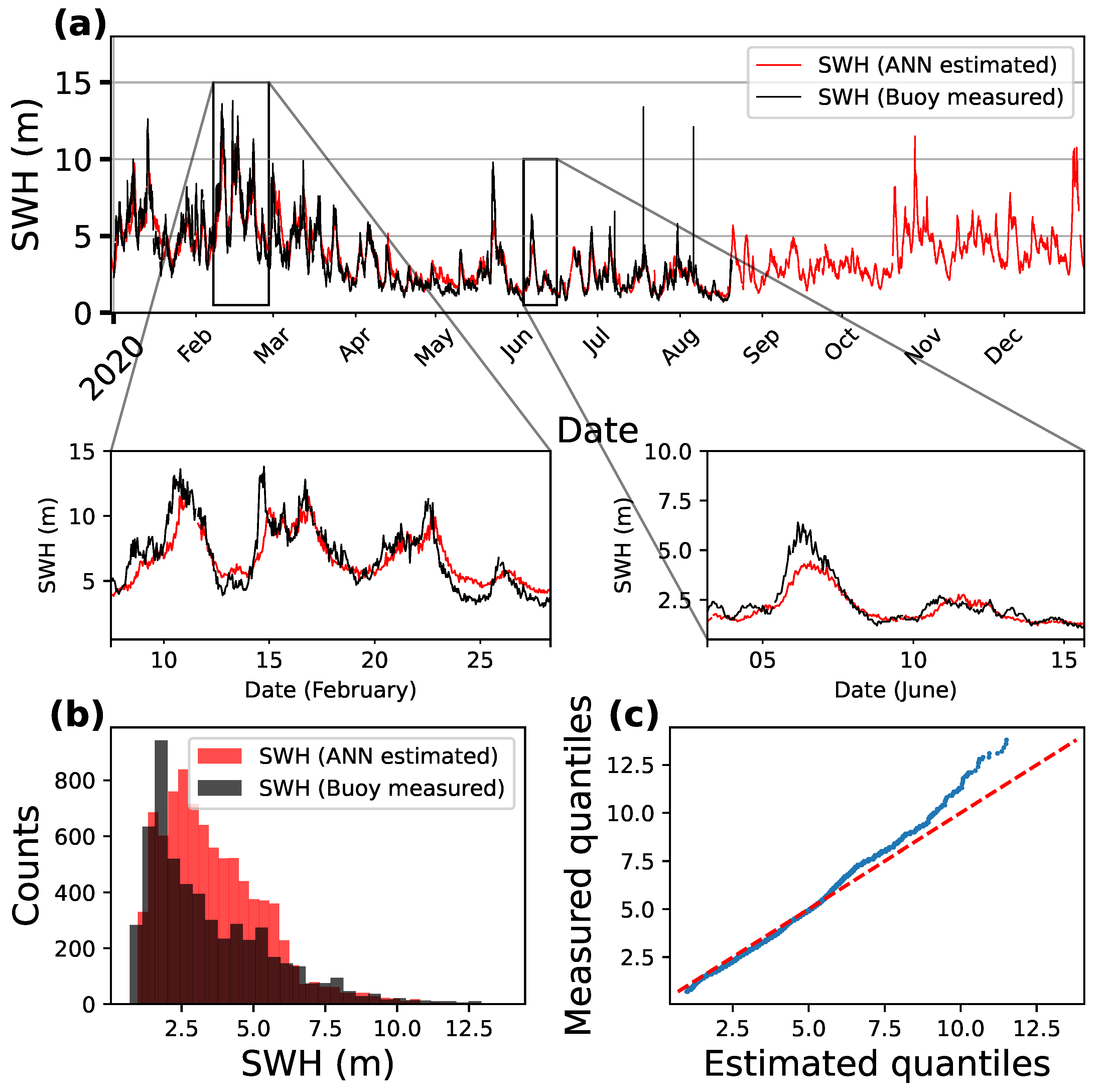
4.1. Trained and Tested Using Buoy SWH Data

In the first scenario, the ANN was trained and validated using microseisms as input and measured SWH data from buoy K4 as the target output (from January 2011 to January 2020). The model was subsequently tested on unseen data from January to December 2020. The time series plot (Figure 5a) compares the predicted/estimated SWH obtained from the ANN model against the measured SWH data from the K4 buoy. The overall agreement is strong, with the model effectively capturing variations in wave height. Zoomed-in insets highlight periods in February and June, showing good correspondence between predicted and measured values across a range of SWHs.

Statistical analysis further supports the model’s performance. The histograms and Q-Q plots (Figure 5b,c) reveal that the ANN-estimated and the observed SWH data share similar statistical distributions, though a slight bias is present for exceptionally large waves. The distributions of both estimated and measured SWH are skewed towards lower values, which is typical for ocean wave height data given the relative excess of smaller waves. The estimated data tend to slightly underrepresent the largest wave heights, giving an apparent increase in the number of mid-range values. Despite this minor discrepancy, the ANN effectively captures the overall wave height distribution, particularly for SWH values below ∼10 m.

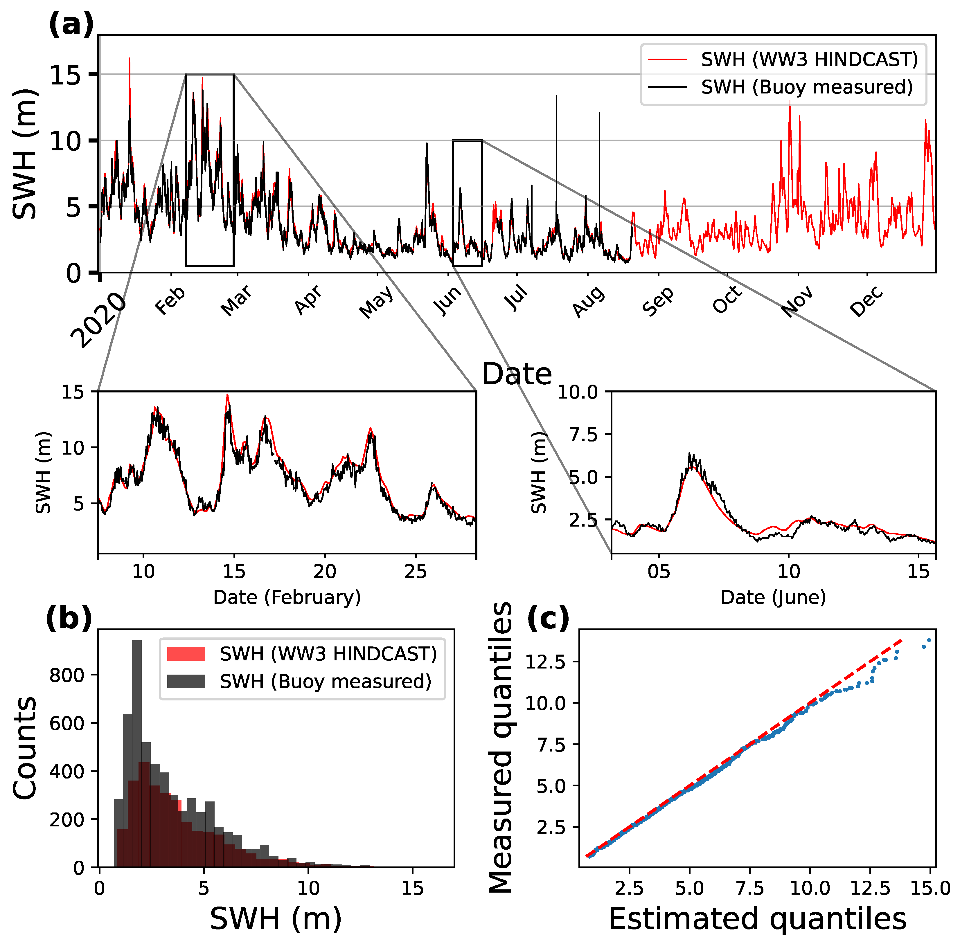
4.2. Buoy Versus Numerical Model Hindcast SWH Data

One limitation of buoy data is the presence of significant data gaps, as illustrated in Figure 4. These gaps arise due to the harsh offshore environment, making buoy data less reliable for continuous ANN training. Furthermore, the spatial sparsity of buoy networks restricts their applicability for broader regional wave estimation. As an alternative, hindcast ocean numerical model data offer a potential solution by providing continuous, spatially extensive wave height estimates. Hindcast models reconstruct past ocean wave conditions based on historical wind and atmospheric data, allowing for accurate wave height predictions. Hence, in this section, we compare measured buoy data to hindcast modelled data, in an effort to assess the quality of the hindcast data as a training set. Note that there is no application of the ANN in Section 4.2.

Figure 6 compares the K4 buoy-measured SWH with hindcast wave model [30] data at the same location. The strong agreement between the two datasets suggests that hindcast SWH data can serve as a viable substitute for buoy measurements in ANN training, particularly in locations with sparse or unreliable buoy coverage.

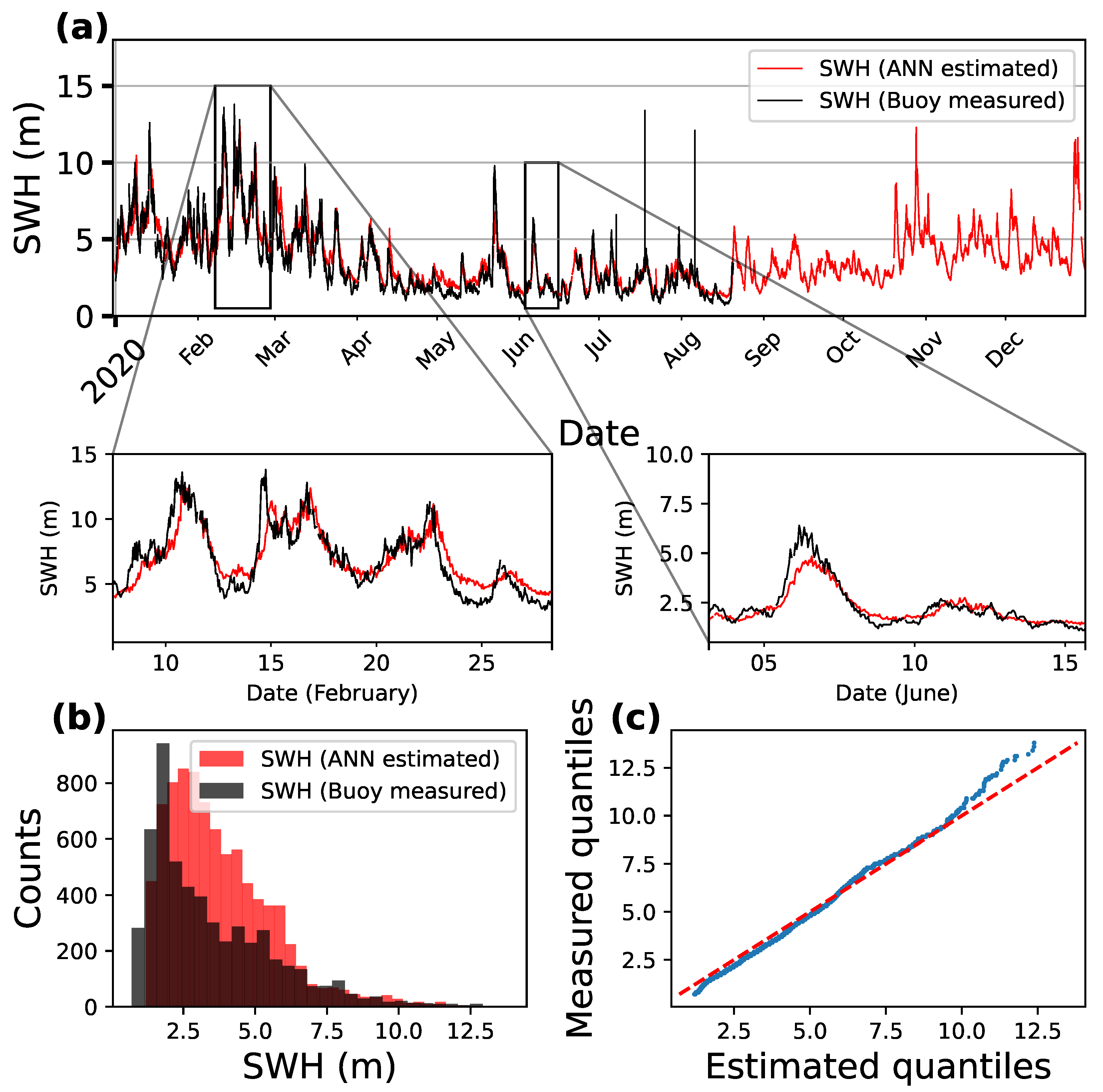
4.3. Trained and Tested Using Numerical Wave Model Hindcast Data

Drawing on the results in Section 4.2, in the second scenario, the ANN was trained using hindcast wave model data at the K4 buoy location. To evaluate its real-world applicability, the trained model was then tested against physical buoy measurements from 2020. That is, we train the ANN using numerical buoy data but test its performance against actual buoy measurements. The results, shown in Figure 7, indicate excellent agreement between the ANN-predicted and buoy-measured SWH values across a broad range of wave heights.

This successful application of the ANN for simulation-to-real data estimation expands the potential of using microseisms for SWH predictions. By leveraging hindcast data for training, the ANN can generalize well to real buoy observations, mitigating the limitations imposed by buoy data gaps and spatial sparsity. The implications of this approach are further discussed in Section 5.

4.4. Statistical Comparison of the ANN Predictions

Although visual inspection demonstrates that the ANN SWH predictions fit the previously unseen observed buoy data well, here, we also undertake a statistical comparison. A statistical assessment of Artificial Neural Network (ANN) predictions is presented in

Table 1. Statistical comparison of ANN predictions with buoy and hindcast data.

	ANN (Trained on Buoy Data) versus Buoy	Hindcast versus Buoy	ANN (Trained on Hindcast Data) versus Buoy
RMSE	0.8780	0.5356	0.9505
MAE	0.6132	0.3394	0.6816
$R^2$	0.8363	0.9426	0.8059
MAPE (%)	19.6353	10.6708	20.2977

. Two scenarios are considered: (i) ANN trained using buoy data versus buoy data, and (ii) ANN trained using hindcast numerical data versus buoy data. Additionally, we show statistical measures of numerically simulated hindcast versus buoy data, for comparison. The Root Mean Square Error (RMSE), the Mean Absolute Error (MAE), the Mean Absolute Percentage Error (MAPE), and the Coefficient of Determination ($R^2$) are all considered. The performance of both trained ANN scenarios is very similar as seen across all statistical measures, with the ANN trained on physical buoy data performing marginally better, as expected. Considering the wave height data ranges of 1.0 m to 12 m, all statistical measures imply fits that are very good to excellent, where RMSE and MAE are both less than 10% of the range and $R^2$ implies that the data variances are well explained. Also, RMSE values are not much greater than MAE values, suggesting that large outliers are not affecting the model. MAPE values of 20% are suggestive of a ‘good prediction’.

5. Discussion and Conclusions

Ocean wave-generated low-frequency seismic waves (microseisms) propagate in the solid Earth at approximately 3.5 km/s. They are continuously generated and clearly detected on terrestrial seismometers inland well beyond the coastal zone. Here, we show that, using an ANN, terrestrial microseism data can be used to estimate ocean SWH, approximately 200 km offshore Ireland in the Northeast Atlantic. The ANN is trained using a combination of seismic and SWH data. The SWH training data take two forms: (i) observed data from buoy K4, and (ii) hindcast modelled wave height data, at the K4 location (see Figure 4). Both approaches demonstrate excellent to very good fits when used to predict previously unseen (by the ANN) buoy wave heights. Hindcast modelled data closely match buoy observations at K4 (see Figure 6), accounting for the excellent ANN performance in predicting buoy-derived SWH even when only trained on hindcast model data. The fits are good up to wave heights of approximately 10 m. Figure 4 shows data availability across the study period. The continuous availability of hindcast modelled SWH data sits in contrast to data dropouts in physical buoy measurements, offering a rich source of the ANN training data. Furthermore, hindcast model data are available at many more points in the ocean than physical buoys, vastly increasing the potential spatial coverage in future applications. Seismic data networks are usually maintained for earthquake monitoring, and in well-maintained networks, data streams are reliable and readily available in real time. For example, at K4, we now have a transfer function from five seismic stations in Ireland that allows for a reliable continuous estimation of wave heights at the K4 location, even when the K4 buoy stops functioning/transmitting (e.g., see Figure 5, mid-August to end-December). As microseisms travel in the ground at approximately 3.5 km/s, they effectively offer a real-time ocean SWH proxy measurement. This suggests a potential complementary, cost-effective, and data-driven approach for future operational applications in the determination of ocean SWH in real time.

The performance of the artificial neural network (ANN) model presented in this study has been evaluated at the K4 buoy location, where it demonstrated promising accuracy in estimating ocean wave heights based on secondary microseisms. However, it is important to note that the model’s success at this specific site does not necessarily guarantee equivalent performance in regions with different bathymetric features, wave climates, or seismic propagation paths. The K4 buoy site, located in a particular oceanic environment with its own set of conditions, offers a unique case for model validation. Therefore, the applicability of the approach we presented herein to other regions with different seismic and oceanographic conditions remains uncertain.

References

1. Bromirski, P.D. Vibrations from the “perfect storm”. Geochem. Geophys. Geosystems 2001, 2, 2000GC000119. [Google Scholar] [CrossRef]
2. Tanimoto, T.; Anderson, A. Seismic noise between 0.003 Hz and 1.0 Hz and its classification. Prog. Earth Planet. Sci. 2023, 10, 56. [Google Scholar] [CrossRef]
3. Li, X.; Xu, Y.; Xie, C.; Sun, S. Global characteristics of ambient seismic noise. J. Seismol. 2022, 26, 343–358. [Google Scholar] [CrossRef]
4. Janssen, T.; Herbers, T.; Battjes, J. Evolution of ocean wave statistics in shallow water: Refraction and diffraction over seafloor topography. J. Geophys. Res. Ocean. 2008, 113, C03024. [Google Scholar] [CrossRef]
5. Chevrot, S.; Sylvander, M.; Benahmed, S.; Ponsolles, C.; Lefèvre, J.; Paradis, D. Source locations of secondary microseisms in western Europe: Evidence for both coastal and pelagic sources. J. Geophys. Res. Solid Earth 2007, 112, B11301. [Google Scholar] [CrossRef]
6. Ardhuin, F.; Gualtieri, L.; Stutzmann, E. How ocean waves rock the Earth: Two mechanisms explain microseisms with periods 3 to 300 s. Geophys. Res. Lett. 2015, 42, 765–772. [Google Scholar] [CrossRef]
7. Farra, V.; Stutzmann, E.; Gualtieri, L.; Schimmel, M.; Ardhuin, F. Ray-theoretical modeling of secondary microseism P waves. Geophys. J. Int. 2016, 206, 1730–1739. [Google Scholar] [CrossRef]
8. Stutzmann, E.; Ardhuin, F.; Schimmel, M.; Mangeney, A.; Patau, G. Modelling long-term seismic noise in various environments. Geophys. J. Int. 2012, 191, 707–722. [Google Scholar] [CrossRef]
9. Kedar, S.; Longuet-Higgins, M.; Webb, F.; Graham, N.; Clayton, R.; Jones, C. The origin of deep ocean microseisms in the North Atlantic Ocean. Proc. R. Soc. A Math. Phys. Eng. Sci. 2008, 464, 777–793. [Google Scholar] [CrossRef]
10. Hasselmann, K. A statistical analysis of the generation of microseisms. Rev. Geophys. 1963, 1, 177–210. [Google Scholar] [CrossRef]
11. Ebeling, C.W. Inferring ocean storm characteristics from ambient seismic noise: A historical perspective. In Advances in Geophysics; Elsevier: Amsterdam, The Netherlands, 2012; Volume 53, pp. 1–33. [Google Scholar]
12. Pellet, L.; Christodoulides, P.; Donne, S.; Bean, C.; Dias, F. Pressure induced by the interaction of water waves with nearly equal frequencies and nearly opposite directions. Theor. Appl. Mech. Lett. 2017, 7, 138–144. [Google Scholar] [CrossRef]
13. Iafolla, L.; Fiorenza, E.; Chiappini, M.; Carmisciano, C.; Iafolla, V.A. Sea wave data reconstruction using micro-seismic measurements and machine learning methods. Front. Mar. Sci. 2022, 9, 798167. [Google Scholar] [CrossRef]
14. Cutroneo, L.; Ferretti, G.; Barani, S.; Scafidi, D.; De Leo, F.; Besio, G.; Capello, M. Near real-time monitoring of significant sea wave height through microseism recordings: Analysis of an exceptional sea storm event. J. Mar. Sci. Eng. 2021, 9, 319. [Google Scholar] [CrossRef]
15. Bensen, G.; Ritzwoller, M.; Barmin, M.; Levshin, A.L.; Lin, F.; Moschetti, M.; Shapiro, N.; Yang, Y. Processing seismic ambient noise data to obtain reliable broad-band surface wave dispersion measurements. Geophys. J. Int. 2007, 169, 1239–1260. [Google Scholar] [CrossRef]
16. Nishida, K. Ambient seismic wave field. Proc. Jpn. Acad. Ser. B 2017, 93, 423–448. [Google Scholar] [CrossRef]
17. Essen, H.H.; Krüger, F.; Dahm, T.; Grevemeyer, I. On the generation of secondary microseisms observed in northern and central Europe. J. Geophys. Res. Solid Earth 2003, 108, 2506. [Google Scholar] [CrossRef]
18. Moni, A.; Craig, D.; Bean, C.J. Separation and location of microseism sources. Geophys. Res. Lett. 2013, 40, 3118–3122. [Google Scholar] [CrossRef]
19. Aster, R.C.; McNamara, D.E.; Bromirski, P.D. Multidecadal climate-induced variability in microseisms. Seismol. Res. Lett. 2008, 79, 194–202. [Google Scholar] [CrossRef]
20. Essen, H.H.; Klussmann, J.; Herber, R.; Grevemeyer, I. Does microseisms in Hamburg (Germany) reflect the wave climate in the North Atlantic? Dtsch. Hydrogr. Z. 1999, 51, 33–45. [Google Scholar] [CrossRef]
21. Ardhuin, F.; Stutzmann, E.; Schimmel, M.; Mangeney, A. Ocean wave sources of seismic noise. J. Geophys. Res. Ocean. 2011, 116, C09004. [Google Scholar] [CrossRef]
22. Beucler, É.; Mocquet, A.; Schimmel, M.; Chevrot, S.; Quillard, O.; Vergne, J.; Sylvander, M. Observation of deep water microseisms in the North Atlantic Ocean using tide modulations. Geophys. Res. Lett. 2015, 42, 316–322. [Google Scholar] [CrossRef]
23. Bromirski, P.D.; Flick, R.E.; Graham, N. Ocean wave height determined from inland seismometer data: Implications for investigating wave climate changes in the NE Pacific. J. Geophys. Res. Ocean. 1999, 104, 20753–20766. [Google Scholar] [CrossRef]
24. Le Pape, F.; Craig, D.; Bean, C.J. How deep ocean-land coupling controls the generation of secondary microseism Love waves. Nat. Commun. 2021, 12, 2332. [Google Scholar] [CrossRef] [PubMed]
25. Le Pape, F.; Bean, C.J. North Atlantic Oscillation (NAO) climate index hidden in ocean generated secondary microseisms. Geophys. Res. Lett. 2021, 48, e2021GL093657. [Google Scholar] [CrossRef]
26. Cannata, A.; Cannavò, F.; Moschella, S.; Di Grazia, G.; Nardone, G.; Orasi, A.; Picone, M.; Ferla, M.; Gresta, S. Unravelling the relationship between microseisms and spatial distribution of sea wave height by statistical and machine learning approaches. Remote Sens. 2020, 12, 761. [Google Scholar] [CrossRef]
27. Donne, S.; Nicolau, M.; Bean, C.; O’Neill, M. Wave height quantification using land based seismic data with grammatical evolution. In Proceedings of the 2014 IEEE Congress on Evolutionary Computation (CEC), Beijing, China, 6–11 July 2014; pp. 2909–2916. [Google Scholar]
28. Longuet-Higgins, M.S. A theory of the origin of microseisms. Philos. Trans. R. Soc. London. Ser. A Math. Phys. Sci. 1950, 243, 1–35. [Google Scholar]
29. UK-MetOffice. Marine Observations—metoffice.gov.uk. Available online: https://www.metoffice.gov.uk/weather/specialist-forecasts/coast-and-sea/observations/ (accessed on 1 June 2024).
30. Laboratoire d’Océanographie Physique et Spatiale (LOPS). LOPS Wave Data. 2024. Available online: https://www.umr-lops.fr/Donnees/Vagues (accessed on 1 June 2024).
31. The MathWorks Inc. Optimization Toolbox Version: 9.4 (R2022b); The MathWorks Inc.: Natick, MA, USA, 2022; Available online: https://www.mathworks.com (accessed on 1 June 2024).
32. Rajurkar, M.; Kothyari, U.; Chaube, U. Artificial neural networks for daily rainfall—Runoff modelling. Hydrol. Sci. J. 2002, 47, 865–877. [Google Scholar] [CrossRef]
33. Dublin Institute for Advanced Studies. Irish National Seismic Network [Data Set]; International Federation of Digital Seismograph Networks: Parkfield, CA, USA, 1993. [Google Scholar] [CrossRef]
Figure 1. (a) Significant Wave Heights (SWHs) recorded by K4 Ocean buoy; (b) seismic displacement recorded by IGLA seismometer in West of Ireland (location shown in Figure 2); and (c) spectrogram of recorded seismic data shown in (b).
Jmse 13 00807 g001
Figure 2. Locations of INSN stations (black inverted triangles) and Ocean buoy K4 (black square).
Jmse 13 00807 g002
Figure 3. Workflow of seismic data processing and ANN model implementation. (a) Pre-processing of seismic data, including denoising and feature extraction. (b) Parameters of Artificial Neural Network (ANN) architecture, detailing network structure, training protocol, and the Bayesian regularization method used for prediction of significant wave height (SWH).
Jmse 13 00807 g003
Figure 4. Data availability from 2011–2021. SMA (see text) is calculated for each seismic station, every hour. Buoy K4 provides a single SWH data point, every hour. The numerical wave model hindcast SWH at the K4 buoy location provides a single data point every three hours [30]. Note that there are considerable data dropouts at physical buoy K4 and at some seismic stations prior to mid-2018 (a complete seismic network upgrade in 2018 has resulted in excellent subsequent up-times for seismic data). SMA data shown still contain earthquake and other disturbances, which were removed before presentation to the ANN.
Jmse 13 00807 g004
Figure 5. (a) Comparison between SWH measured by K4 buoy and estimated SWH (at K4’s location), using the ANN with microseisms as input. (b) histograms of observed and predicted SWH data, and (c) quantile–quantile plot comparing the two datasets. The red dotted line in (c) represents the 45-degree reference line, indicating a perfect match between the theoretical and observed quantiles. The blue line shows the actual data comparison. Deviations from the red line indicate differences between the distributions. Note that there are no data available from the buoy from mid-August; however, the ANN continues to give an SWH estimate through the seismic data proxy.
Jmse 13 00807 g005
Figure 6. (a) K4 buoy versus hindcast ocean wave model SWH data at K4 location. Buoy data are sampled every hour. Hindcast data are sampled every three hours, accounting for the fewer data points seen in histogram in (b); however, histograms broadly have same shape; (c) quantile–quantile plot. The red dotted line in (c) represents the 45-degree reference line, indicating a perfect match between the theoretical and observed quantiles. The blue line shows the actual data comparison. Deviations from the red line indicate differences between the distributions.
Jmse 13 00807 g006
Figure 7. (a) Comparison between SWH measured by K4 buoy and estimated SWH (at K4’s location), employing the ANN trained using numerical wave model hindcast data. (b) Histograms of observed and predicted SWH data, and (c) quantile-quantile plot comparing the two datasets showing an excellent match up to 10 m. The red dotted line in (c) represents the 45-degree reference line, indicating a perfect match between the theoretical and observed quantiles. The blue line shows the actual data comparison. Deviations from the red line indicate differences between the distributions. Note that there are no data available from the buoy from mid-August; however, the ANN continues to give an SWH estimate through the seismic data proxy.
Jmse 13 00807 g007