Research on Characteristics of the Hermite–Gaussian Correlated Vortex Beam

Abstract

In this work, a new beam named the Hermite–Gaussian correlated vortex beam (HGCVB) is introduced. The intensity and coherence of this HGCVB in oceanic turbulence are analyzed. The results show that the HGCVB displays a splitting property during propagation, and the HGCVB can evolve into the array profile with hollow center beamlets. The results display that the evolution of the intensity of the HGCVB is manipulated by the coherence length δ₀ and topological charge M. Meanwhile, the array distribution of coherence of the HGCVB in oceanic turbulence can evolve into a one-spot pattern on propagation. The results show that this HGCVB evolves from a Gaussian beam into a beam array composed of beamlets with hollow centers and may have a potential application in oceanic turbulence.

1. Introduction

The properties of light propagating in an underwater environment determine the performance of underwater optical systems [1,2]. Until now, the influences of oceanic turbulence on the characteristics of light have been widely viewed. The scintillation indexes of spherical wave [3], partially coherent flat-topped beam [4], and lidar [5] in oceanic turbulence have been investigated. The structure function [6], intensity [7,8], arrival fluctuations [9], and Bit error rate [10] of beams in oceanic turbulence have been widely studied. In addition, the evolution of chirped pulsed beams in the ocean has been analyzed [11,12]. For underwater communication, the performance of wireless optical communication has been studied [13,14].

On the other hand, the properties of the partially coherent beam (PCB) can be manipulated by coherence function [15], and the PCBs are beneficial for turbulent environments. Thus, the PCBs correlated with different coherent functions have been introduced and studied in oceanic turbulence, such as the Gaussian–Schell model (GSM) beam [16], PCB with double vortex [17], optical coherence lattice [18], electromagnetic multi-GSM vortex beam [19], rectangular Hermite–Gaussian beam array [20], and multi-GSM beam array [21]. Moreover, PCBs correlated with special coherence functions have been proposed and studied, due to their unique properties, such as the Laguerre–Gaussian correlated (LGC) beam [22,23], LGC vortex beam [24,25], multi-Gaussian–Schell model (MGSM) beam [26], and MGSM vortex beam [27]. Recently, a new PCB named the Hermite–Gaussian correlated (HGC) beam [28] has been introduced. The HGC beam with a twisted phase is introduced [29], and the non-uniform factor is also introduced into the HGC beam [30]. However, the HGC beam with the vortex phase has not been viewed. In this work, the vortex phase is introduced into the HGC beam, and a new beam named the Hermite–Gaussian correlated vortex beam (HGCVB) is produced. The cross-spectral density (CSD) of the HGCVB in anisotropic oceanic turbulence is derived. The intensity and coherence properties are illustrated and discussed based on the numerical simulations. In Section 2, the CSD of the HGCVB is presented, and the propagation CSD of the HGCVB in oceanic turbulence is derived. In Section 3, the intensity and coherence of the HGCVB are analyzed. The conclusions are summarized in Section 4.

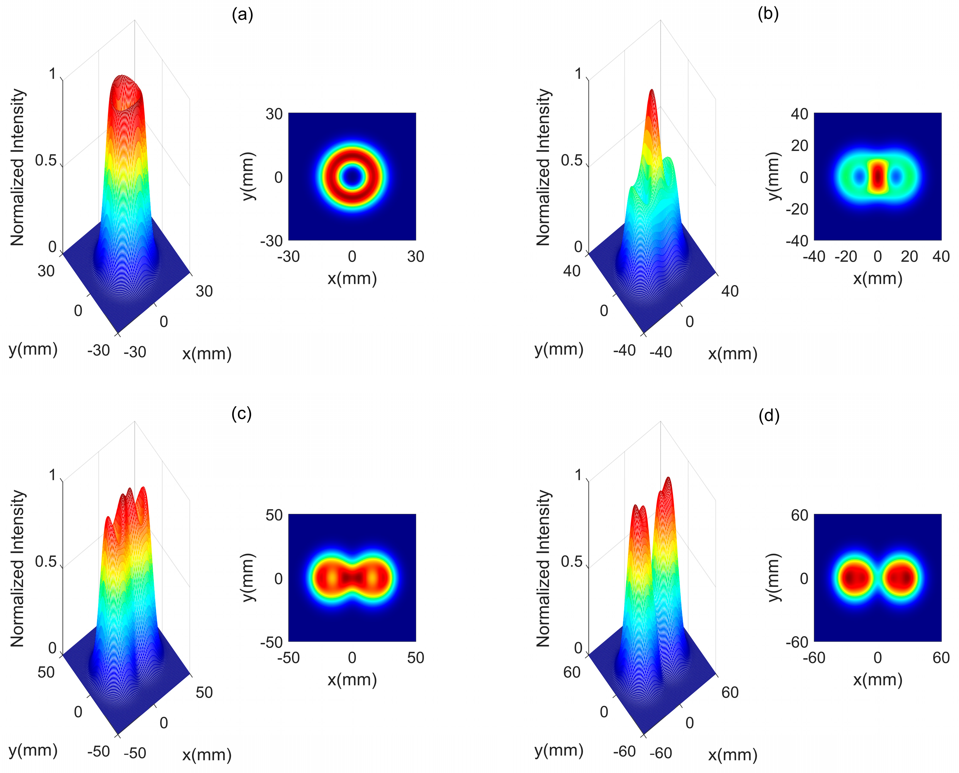
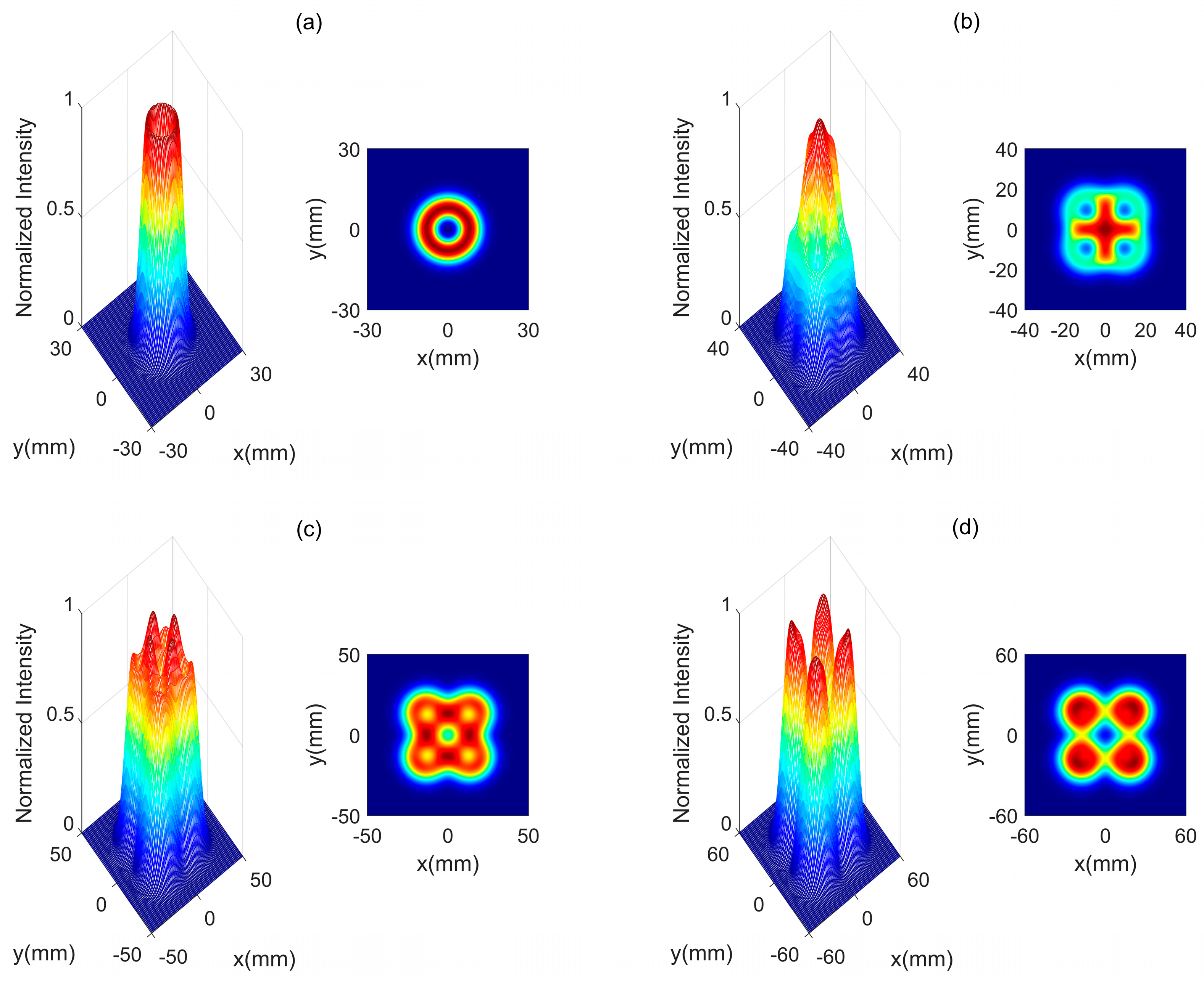
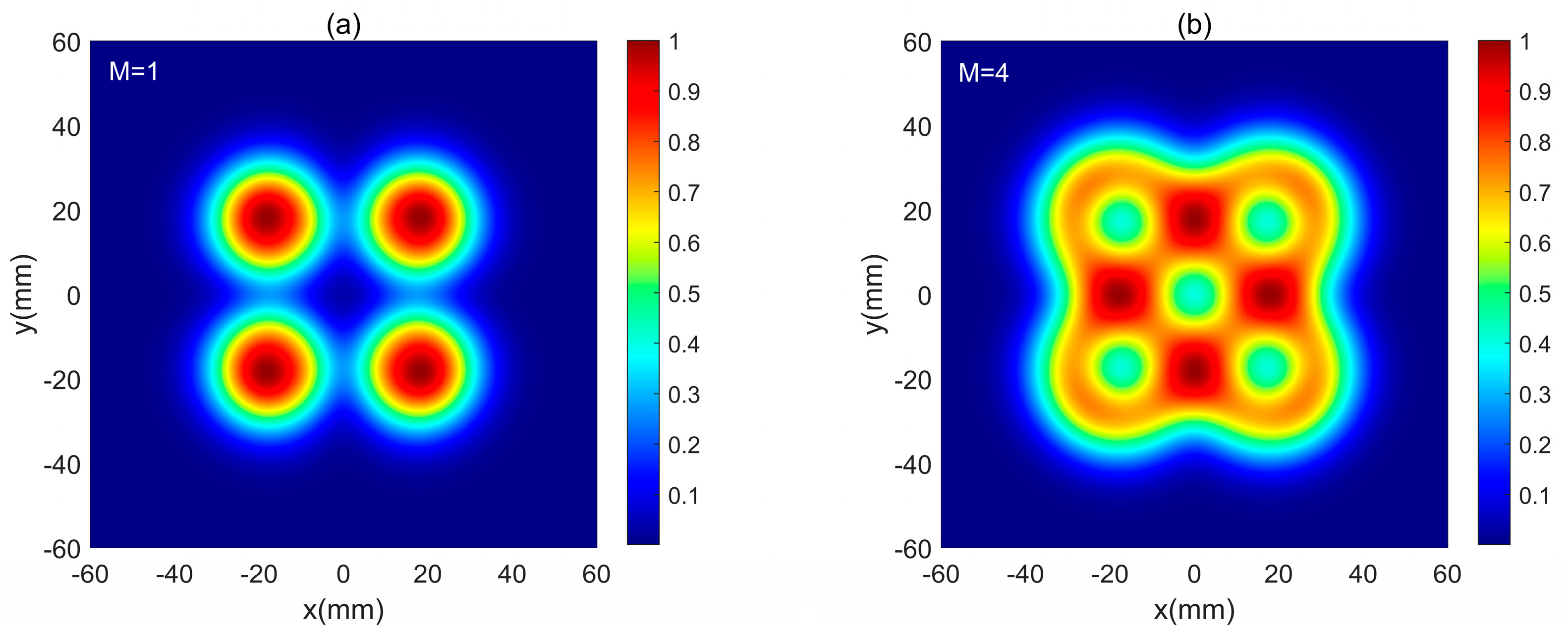
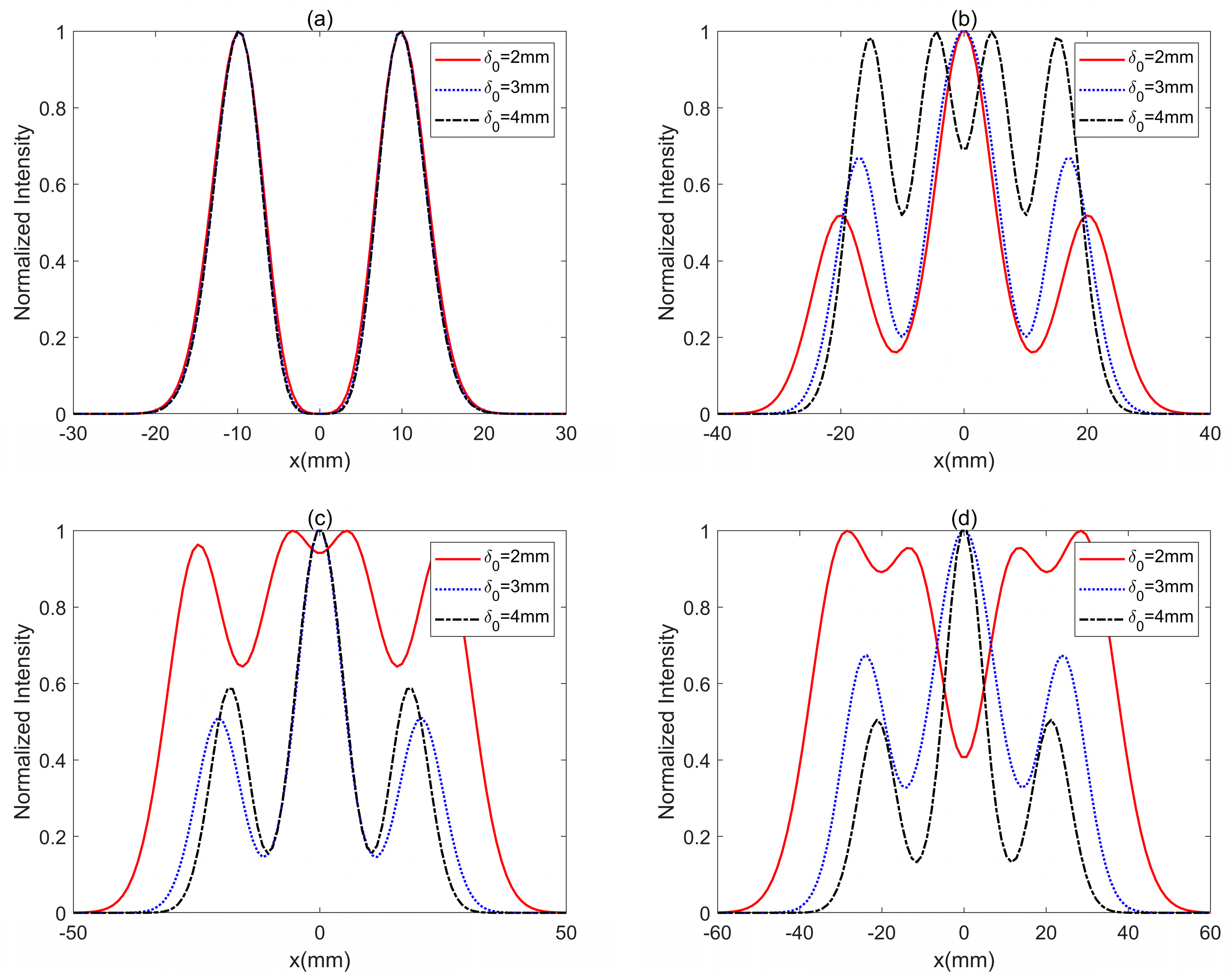
2. Propagation of the HGCVB in Oceanic Turbulence

Recalling the model of the HGC beam introduced by Cai et al. [28], when the vortex phase is added to the HGC beam, the CSD of the HGCVB can be written as:

$$\begin{array}{l}W\left({\mathbf{r}}_1,{\mathbf{r}}_2,0\right)=G_0{\displaystyle \frac{1}{H_{2m}\left(0\right)}}{\displaystyle \frac{1}{H_{2n}\left(0\right)}}\exp \left(-{\displaystyle \frac{{\mathbf{r}}_1^2+{\mathbf{r}}_2^2}{4w_0^2}}\right)H_{2m}\left({\displaystyle \frac{x_2-x_1}{\sqrt{2}{\delta }_{0x}}}\right)\exp \left[-{\displaystyle \frac{{\left(x_2-x_1\right)}^2}{2{\delta }_{0x}^2}}\right]\\ H_{2n}\left({\displaystyle \frac{y_2-y_1}{\sqrt{2}{\delta }_{0y}}}\right)\exp \left[-{\displaystyle \frac{{\left(y_2-y_1\right)}^2}{2{\delta }_{0y}^2}}\right]{\left(x_1+i{y}_1\right)}^M{\left(x_2-i{y}_2\right)}^M\end{array}$$

(1)

where $G_0$ is the constant, $M$ is the topological charge, ${\delta }_{0x}$ and ${\delta }_{0y}$ are the coherence length, and $H$ is the Hermite polynomial and can be given as [31]:

$$H_n\left(x\right)={\displaystyle \sum _{l=0}^{\left[n/2\right]}\frac{{\left(-1\right)}^{l}n!}{l!\left(n-2l\right)!}}{\left(2x\right)}^{n-2l}$$

(2)

When $M=0$ in Equation (1), the CSD of the HGCVB will reduce to the HGC beam.

Considering the generalized Huygens–Fresnel integral, the CSD of the HGCVB in anisotropic oceanic turbulence can be described by [3,4,5,6,7,8,9,10]:

$$\begin{array}{l}W\left({\mathbf{\rho }}_1,{\mathbf{\rho }}_2,z\right)={\displaystyle \frac{k^2}{4{\pi }^2{z}^2}}{\displaystyle \iint d{\mathbf{r}}_{1}d{\mathbf{r}}_{2}W\left({\mathbf{r}}_1,{\mathbf{r}}_2,0\right)}\\ \times \exp \left[-{\displaystyle \frac{ik}{2z}}{\left({\mathbf{\rho }}_1-{\mathbf{r}}_1\right)}^2+{\displaystyle \frac{ik}{2z}}{\left({\mathbf{\rho }}_2-{\mathbf{r}}_2\right)}^2\right]〈\exp \left[\psi \left({\mathbf{r}}_1,{\mathbf{\rho }}_1\right)+{\psi }^{\ast }\left({\mathbf{r}}_2,{\mathbf{\rho }}_2\right)\right]〉\end{array}$$

(3)

with

$$〈\exp \left[\psi \left({\mathbf{r}}_1,{\mathbf{\rho }}_1\right)+{\psi }^{\ast }\left({\mathbf{r}}_2,{\mathbf{\rho }}_2\right)\right]〉=\exp \left[-{\displaystyle \frac{{\left({\mathbf{r}}_1-{\mathbf{r}}_2\right)}^2+\left({\mathbf{r}}_1-{\mathbf{r}}_2\right)\left({\mathbf{\rho }}_1-{\mathbf{\rho }}_2\right)+{\left({\mathbf{\rho }}_1-{\mathbf{\rho }}_2\right)}^2}{T^2}}\right]$$

(4)

where $T$ can be given as [32,33]

$$T={\left[8.705\times {10}^{-8}{k}^{2}z{\left(\epsilon \eta \right)}^{-1/3}{\zeta }^{-2}{\chi }_T\left(1-2.605{\varpi }^{-1}+7.007{\varpi }^{-2}\right)\right]}^{-1/2}$$

(5)

where $\zeta$ is the anisotropic factor, $\eta$ represents the inner scale, $\varpi$ denotes the ratio of temperature and salinity, $\epsilon$ is the dissipation rate of fluid, and $x_T$ gives the dissipation of temperature.

Recalling the following expressions [31]:

$${\left(x+y\right)}^l={\displaystyle \sum _{h=0}^l\frac{l!}{h!\left(l-h\right)!}{x}^{l-h}{y}^h}$$

(6)

$${\displaystyle {\int }_{-\infty }^{+\infty }{x}^n\exp \left[-{\left(x-\beta \right)}^2\right]dx}={\left(2i\right)}^{-n}\sqrt{\pi }{H}_n\left(i\beta \right)$$

(7)

Substituting Equations (1) and (4) into Equation (3), the CSD of the HGCVB in an anisotropic oceanic turbulence can be derived as:

$$\begin{array}{l}W\left({\mathbf{\rho }}_1,{\mathbf{\rho }}_2,z\right)={\displaystyle \frac{k^2}{4{\pi }^2{z}^2}}\exp \left[-{\displaystyle \frac{ik}{2z}}\left({\mathbf{\rho }}_1^2-{\mathbf{\rho }}_2^2\right)\right]\exp \left[-{\displaystyle \frac{{\left({\rho }_{1x}-{\rho }_{2x}\right)}^2+{\left({\rho }_{1y}-{\rho }_{2y}\right)}^2}{T^2}}\right]\\ G_0{\displaystyle \frac{1}{H_{2m}\left(0\right)}}{\displaystyle \frac{1}{H_{2n}\left(0\right)}}{\displaystyle \sum _{h_1=0}^M\left(\begin{array}{c}M\\ h_1\end{array}\right)i^{h_1}}{\displaystyle \sum _{h_2=0}^M\left(\begin{array}{c}M\\ h_2\end{array}\right){\left(-i\right)}^{h_2}}\\ {\displaystyle \sum _{l_x=0}^m\frac{{\left(-1\right)}^{l_x}\left(2m\right)!}{l_x!\left(2m-2l_x\right)!}}{\left({\displaystyle \frac{2}{\sqrt{2}{\delta }_{0x}}}\right)}^{2m-2l_x}{\displaystyle \sum _{l_y=0}^n\frac{{\left(-1\right)}^{l_y}\left(2n\right)!}{l_y!\left(2n-2l_y\right)!}}{\left({\displaystyle \frac{2}{\sqrt{2}{\delta }_{0y}}}\right)}^{2n-2l_y}\\ W\left({\rho }_x,z\right)W\left({\rho }_y,z\right)\end{array}$$

(8)

where

$$\begin{array}{l}W\left({\rho }_x,z\right)={\displaystyle \sum _{s_x=0}^{2m-2l_x}\frac{\left(2m-2l_x\right)!{\left(-1\right)}^{s_x}}{s_x!\left(2m-2l_x-s_x\right)!}}\sqrt{{\displaystyle \frac{\pi }{a_x}}}\left(M-h_1+s_x\right)!{\left({\displaystyle \frac{1}{a_x}}\right)}^{M-h_1+s_x}\exp \left[{\displaystyle \frac{1}{a_x}}{\left({\displaystyle \frac{ik}{2z}}{\rho }_{1x}-{\displaystyle \frac{{\rho }_{1x}-{\rho }_{2x}}{2T^2}}\right)}^2\right]\\ {\displaystyle \sum _{t_x=0}^{\left[\frac{M-h_1+s_x}{2}\right]}\frac{1}{t_x!\left(M-h_1+s_x-2t_x\right)!}}{\left({\displaystyle \frac{a_x}{4}}\right)}^{t_x}{\displaystyle \sum _{d_x=0}^{\left[M-h_1+s_x-2t_x\right]}\left(\begin{array}{c}M-h_1+s_x-2t_x\\ d_x\end{array}\right)}{\left({\displaystyle \frac{ik}{2z}}{\rho }_{1x}-{\displaystyle \frac{{\rho }_{1x}-{\rho }_{2x}}{2T^2}}\right)}^{M-h_1+s_x-2t_x-d_x}\\ {\left({\displaystyle \frac{1}{2{\delta }_{0x}^2}}+{\displaystyle \frac{1}{T^2}}\right)}^{d_x}\sqrt{{\displaystyle \frac{\pi }{b_x}}}{\left({\displaystyle \frac{i}{2\sqrt{b_x}}}\right)}^{M-h_2+2m-2l_x-s_x+d_x}\exp \left({\displaystyle \frac{c_x^2}{b}}\right)H_{M-h_2+2m-2l_x-s_x+d_x}\left(-{\displaystyle \frac{i{c}_x}{\sqrt{b_x}}}\right)\end{array}$$

(9)

$$\begin{array}{l}W\left({\rho }_y,z\right)={\displaystyle \sum _{s_y=0}^{2n-2l_y}\frac{\left(2n-2l_y\right)!{\left(-1\right)}^{s_y}}{s_y!\left(2n-2l_y-s_y\right)!}}\sqrt{{\displaystyle \frac{\pi }{a_y}}}\left(h_1+s_y\right)!{\left({\displaystyle \frac{1}{a_y}}\right)}^{h_1+s_y}\exp \left[{\displaystyle \frac{1}{a_y}}{\left({\displaystyle \frac{ik}{2z}}{\rho }_{1y}-{\displaystyle \frac{{\rho }_{1y}-{\rho }_{2y}}{2T^2}}\right)}^2\right]\\ {\displaystyle \sum _{t_y=0}^{\left[\frac{h_1+s_y}{2}\right]}\frac{1}{t_y!\left(h_1+s_y-2t_y\right)!}}{\left({\displaystyle \frac{a_y}{4}}\right)}^{t_x}{\displaystyle \sum _{d_y=0}^{h_1+s_y-2t_y}\left(\begin{array}{c}{h}_1+s_y-2t_y\\ d_y\end{array}\right)}{\left({\displaystyle \frac{ik}{2z}}{\rho }_{1y}-{\displaystyle \frac{{\rho }_{1y}-{\rho }_{2y}}{2T^2}}\right)}^{h_1+s_y-2t_y-d_y}{\left({\displaystyle \frac{1}{2{\delta }_{0y}^2}}+{\displaystyle \frac{1}{T^2}}\right)}^{d_y}\\ \sqrt{{\displaystyle \frac{\pi }{b_y}}}{\left({\displaystyle \frac{i}{2\sqrt{b_y}}}\right)}^{h_2+2n-2l_y-s_y+d_y}\exp \left({\displaystyle \frac{c_y^2}{b}}\right)H_{h_2+2n-2l_y-s_y+d_y}\left(-{\displaystyle \frac{i{c}_y}{\sqrt{b_y}}}\right)\end{array}$$

(10)

with

$$a_{\beta }={\displaystyle \frac{1}{4w_0^2}}+{\displaystyle \frac{1}{2{\delta }_{0\beta }^2}}+{\displaystyle \frac{1}{T^2}}+{\displaystyle \frac{ik}{2z}}\left(\beta =x,y\right)$$

(11)

$$b_{\beta }={\displaystyle \frac{1}{4w_0^2}}+{\displaystyle \frac{1}{2{\delta }_{0\beta }^2}}+{\displaystyle \frac{1}{T^2}}-{\displaystyle \frac{ik}{2z}}-{\displaystyle \frac{1}{a_{\beta }}}{\left({\displaystyle \frac{1}{2{\delta }_{0\beta }^2}}+{\displaystyle \frac{1}{T^2}}\right)}^2$$

(12)

$$c_x=-{\displaystyle \frac{ik}{2z}}{\rho }_{2x}+{\displaystyle \frac{{\rho }_{1x}-{\rho }_{2x}}{2T^2}}+{\displaystyle \frac{1}{a_x}}\left({\displaystyle \frac{1}{2{\delta }_{0x}^2}}+{\displaystyle \frac{1}{T^2}}\right)\left({\displaystyle \frac{ik}{2z}}{\rho }_{1x}-{\displaystyle \frac{{\rho }_{1x}-{\rho }_{2x}}{2T^2}}\right)$$

(13)

$$c_y=-{\displaystyle \frac{ik}{2z}}{\rho }_{2y}+{\displaystyle \frac{{\rho }_{1y}-{\rho }_{2y}}{2T^2}}+{\displaystyle \frac{1}{a_y}}\left({\displaystyle \frac{1}{2{\delta }_{0y}^2}}+{\displaystyle \frac{1}{T^2}}\right)\left({\displaystyle \frac{ik}{2z}}{\rho }_{1y}-{\displaystyle \frac{{\rho }_{1y}-{\rho }_{2y}}{2T^2}}\right)$$

(14)

The intensity and degree of coherence (DOC) of the HGCVB can be described by [34]:

$$I\left(\mathbf{\rho },z\right)=W\left(\mathbf{\rho },\mathbf{\rho },z\right)$$

(15)

$$\mu \left({\mathbf{\rho }}_1,{\mathbf{\rho }}_2,z\right)={\displaystyle \frac{W\left({\mathbf{\rho }}_1,{\mathbf{\rho }}_2,z\right)}{\sqrt{W\left({\mathbf{\rho }}_1,{\mathbf{\rho }}_1,z\right)W\left({\mathbf{\rho }}_2,{\mathbf{\rho }}_2,z\right)}}}$$

(16)

3. Results and Analysis

Here, the characteristics (intensity and DOC) of the HGCVB have been viewed and analyzed. The wavelength is set as $\lambda =532 \mathrm{nm}$, ${\delta }_{0x}={\delta }_{0y}={\delta }_0=2 \mathrm{mm}$, $M=2$, $\epsilon =1\times {10}^{-7}{\mathrm{m}}^{-3}/{\mathrm{s}}^2$, $\eta =1 \mathrm{mm}$, and $\varpi =-2.5$ in numerical calculation.

First, the intensity of the HGCVB with $w_0=5 \mathrm{mm}$, $m=3$, and $n=0$ in free space is illustrated in Figure 1. The HGCVB retains the hollow center shape of the vortex beam at a short distance (Figure 1a). The HGCVB will lose the ring shape and split as $z$ increases (Figure 1b), and the splitting characteristic is caused by the HGC source. The intensity of this HGCVB can split into two spots with a hollow center at $z=150 \mathrm{m}$ (Figure 1c). As $z$ increases, the two beamlets of the HGCVB will gradually lose the ring shape, and the intensity of this HGCVB will split into two spots (Figure 1d). In Figure 1, the phenomenon of the HGCVB with $m=3$ and $n=0$ evolving from a spot pattern into two spots is caused by the HGC function, and this splitting phenomenon is in accordance with the HGC beam [28].

When the parameters $m$ and $n$ of the HGCVB change, Figure 2 illustrates the intensity of the HGCVB with $w_0=4 \mathrm{mm}$, $m=n=2$ in free space. The ring shape of this HGCVB with $m=n=2$ can be retained at $z=10 \mathrm{m}$ (Figure 2a). This HGCVB with $m=n=2$ will split along the x and y axes (Figure 2b), and this HGCVB can gradually split into four beamlets with hollow centers (Figure 2c), while the HGC beam just splits into four beamlets [28]. At $z=200 \mathrm{m}$, the intensity of this HGCVB will become four spots (Figure 2d). From Figure 1 and Figure 2, one sees that the splitting phenomenon is manipulated by $m$ and $n$ of the HGC source, and the number of splitting beamlets is the same as the results of the HGC beam [28]. When $M$ changes, the intensity of the HGCVB with $M=1$ and $m=n=2$ in free space at $z=200 \mathrm{m}$ will show the four beamlets with a Gauss distribution (Figure 3a). However, the HGCVB with $M=4$ and $m=n=2$ in free space at $z=200 \mathrm{m}$ will show the four beamlets with hollow profiles (Figure 3b). From Figure 2d and Figure 3a,b, one concludes that the larger $M$ of the HGCVB is beneficial for the beamlets retaining the hollow center.

The effects of ${\delta }_0$ and $M$ are analyzed in Figure 4 and Figure 5. The intensity (y = 0) of the HGCVB with $w_0=4 \mathrm{mm}$, $M=3$, $m=3$, and $n=0$ in free space for the different ${\delta }_0$ is illustrated in Figure 4. These HGCVBs with the different ${\delta }_0$ have the same ring distribution at the short distance (Figure 4a). As $z$ increases, the smaller ${\delta }_0$ of the HGCVB is beneficial for the splitting phenomenon (Figure 4b). The intensity of the HGCVB with larger ${\delta }_0=4 \mathrm{mm}$ can also lose the ring shape at $z=150 \mathrm{m}$ (Figure 4c), and the HGCVBs can split into two points at $z=200\mathrm{m}$ (Figure 4d). Figure 5 shows the intensity (y = 0) of the HGCVB with $w_0=4 \mathrm{mm}$, ${\delta }_0=2 \mathrm{mm}$, $m=3$, and $n=0$ in free space for the different $M$. At $z=10 \mathrm{m}$, the intensity profiles of these HGCVBs with the different $M$ have the same ring distribution (Figure 5a). As $z$ increases, these HGCVBs will split, and the HGCVB with the larger $M$ will have a larger width (Figure 5b), and the beamlets of the HGCVB with the larger $M$ can show a ring pattern (Figure 5c). At $z=200 \mathrm{m}$, the HGCVB with the larger $M$ will split into two beamlets, and the HGCVB with $M=1$ will show the one-spot pattern (Figure 5d). Therefore, the splitting beamlets can be determined by $M$ and the HGCVB with a larger $M$ is beneficial for the splitting phenomenon.

Next, the characteristics of the HGCVB in anisotropic oceanic turbulence are discussed. The evolution of the HGCVB with $w_0=4 \mathrm{mm}$, $M=2$, and $m=n=2$ in oceanic turbulence with $\varsigma =2$ and $x_T=1\times {10}^{-8} {\mathrm{K}}^2/\mathrm{s}$ is given in Figure 6. At short distances, the HGCVB in oceanic turbulence retains the same ring shape as the HGCVB in free space (comparing Figure 6a with Figure 2a). As $z$ increases, this HGCVB in oceanic turbulence will spread, but the splitting phenomenon of this HGCVB in oceanic turbulence disappears (Figure 6b), while the same HGCVB in free space shows the splitting property (Figure 2b). As $z$ increases to $z=150 \mathrm{m}$, this HGCVB, through oceanic turbulence, will become a one-spot pattern (Figure 6c), while the same HGCVB in free space splits into four beamlets with a hollow center (Figure 2c). At $z=200 \mathrm{m}$, this HGCVB in oceanic turbulence will spread and retain the one-spot pattern (Figure 6d). From Figure 2d and Figure 6d, one concludes that the oceanic turbulence will cause the beamlets to evolve into one spot.

To view the influences of the strength of oceanic turbulence on the propagation of the HGCVB, the intensity of the HGCVB with $w_0=4 \mathrm{mm}$, $M=2$, and $m=n=2$ in oceanic turbulence with $\varsigma =2$ for the different $x_T$ was measured. The intensity of this HGCVB in oceanic turbulence with smaller $x_T=1\times {10}^{-8}{\mathrm{K}}^2/\mathrm{s}$ will show the array profile with four beamlets (Figure 7a), while the same HGCVB in oceanic turbulence with $x_T=1\times {10}^{-7}{\mathrm{K}}^2/\mathrm{s}$ will turn into one spot (Figure 7b). From Figure 6b and Figure 7a,b, one can conclude that the oceanic turbulence with larger $x_T$ will cause the HGCVB to lose beamlets faster. Figure 8 shows the intensity of the HGCVB with $w_0=4 \mathrm{mm}$, $M=2$, and $m=n=2$ in oceanic turbulence with $x_T=5\times {10}^{-8}{\mathrm{K}}^2/\mathrm{s}$ for the different $\varsigma$. This HGCVB in oceanic turbulence with $\varsigma =3$ will split four beamlets (Figure 8a), while the same HGCVB in oceanic turbulence with $\varsigma =1$ will become one spot (Figure 8b). Therefore, the HGCVB in anisotropic oceanic turbulence with larger $x_T$ or smaller $\varsigma$ will lose the array profile and evolve into a one-spot pattern faster.

Lastly, the DOC of the HGCVB is investigated. Figure 9 illustrates the DOC of the HGCVB with $w_0=4 \mathrm{mm}$, $M=2$, and $m=n=2$ in free space. At a short distance, the DOC of this HGCVB in free space will show the multi-point distribution (Figure 9a), and the DOC will evolve into an array distribution as $z$ increases (Figure 9b). When the same HGCVB is in oceanic turbulence with $\varsigma =2$ and $x_T=5\times {10}^{-8}{\mathrm{K}}^2/\mathrm{s}$, the DOC distribution of the HGCVB is similar to that in free space at $z=10 \mathrm{m}$ (Figure 10a). However, the DOC of this HGCVB in oceanic turbulence will show the one-spot distribution (Figure 10b). Therefore, the DOC of the HGCVB in oceanic turbulence will gradually be destroyed on propagation.

4. Conclusions

In this study, we have introduced a new theoretical model of the HGCVB, and this HGCVB is correlated with the HGC source. The CSD of the HGCVB in oceanic turbulence is derived based on the generalized Huygens–Fresnel integral. The intensity of this HGCVB in free space will evolve from a ring shape into an array profile with hollow center beamlets, and the HGCVB will turn into an array beam during propagation. It is found that the HGCVB with a larger $M$ can retain the array profile with hollow beamlets better at longer distances, and the smaller ${\delta }_0$ is beneficial for the generation of the array profile. In addition, the HGCVB in anisotropic oceanic turbulence with larger $x_T$ or smaller $\varsigma$ will lose the array profile and evolve into a Gaussian-like beam faster. The array distribution of the DOC of the HGCVB in oceanic turbulence can gradually be destroyed on propagation. The results provide a new way to generate an array beam with hollow center beamlets.

References

1. Baykal, Y.; Ata, Y.; Gökçe, M.C. Underwater turbulence, its effects on optical wireless communication and imaging: A review. Opt. Laser Technol. 2022, 156, 108624. [Google Scholar] [CrossRef]
2. Korotkova, O. Light Propagation in a Turbulent Ocean. Prog. Opt. 2019, 64, 1–43. [Google Scholar]
3. Baykal, Y. Scintillation index in strong oceanic turbulence. Opt. Commun. 2016, 375, 15–18. [Google Scholar] [CrossRef]
4. Yousefi, M.; Golmohammady, S.; Mashal, A.; Kashani, F.D. Analyzing the propagation behavior of scintillation index and bit error rate of a partially coherent flat-topped laser beam in oceanic turbulence. J. Opt. Soc. Am. A Opt. Image Sci. Vis. 2015, 32, 1982–1992. [Google Scholar] [CrossRef] [PubMed]
5. Gerçekcioğlu, H.; Baykal, Y. Laser beam scintillations of LIDAR operating in weak oceanic turbulence. J. Opt. Soc. Am. B 2022, 40, A44–A50. [Google Scholar] [CrossRef]
6. Ata, Y. Structure function, coherence length, and angle-of-arrival variance for Gaussian beam propagation in turbulent waters. J. Opt. Soc. Am. A Opt. Image Sci. Vis. 2022, 39, 63–71. [Google Scholar] [CrossRef]
7. Bayraktar, M. Average intensity of astigmatic hyperbolic sinusoidal Gaussian beam propagating in oceanic turbulence. Phys. Scr. 2020, 96, 025501. [Google Scholar] [CrossRef]
8. Liu, L.; Liu, Y.; Chang, H.; Huang, J.; Zhu, X.; Cai, Y.; Yu, J. Second-Order Statistics of Self-Splitting Structured Beams in Oceanic Turbulence. Photonics 2023, 10, 339. [Google Scholar] [CrossRef]
9. Yi, X.; Ban, K.; Liu, H.; Ata, Y.; Cheng, M.; Zhang, L. Aperture-Averaged Angle-of-Arrival Fluctuations in Oceanic Turbulence of Arbitrary Strength. IEEE Trans. Antennas Propag. 2024, 72, 2631–2642. [Google Scholar] [CrossRef]
10. Gerçekcioğlu, H.; Baykal, Y. Bit error rate of M-pulse position modulated laser beams for vertical links operating in weak oceanic turbulence. J. Opt. 2024, 26, 105602. [Google Scholar] [CrossRef]
11. Jo, J.-H.; Ri, O.-H.; Ju, T.Y.; Pak, K.-M.; Ri, S.-G.; Hong, K.-C.; Hyon Jang, S. Effect of oceanic turbulence on the spectral changes of diffracted chirped Gaussian pulsed beam. Opt. Laser Technol. 2022, 153, 108200. [Google Scholar] [CrossRef]
12. Liu, D.J.; Wang, Y.C.; Wang, G.Q.; Yin, H.M.; Wang, J.R. The influence of oceanic turbulence on the spectral properties of chirped Gaussian pulsed beam. Opt. Laser Technol. 2016, 82, 76–81. [Google Scholar] [CrossRef]
13. Ata, Y.; Baykal, Y.; Gökçe, M.C. Analysis of Optical Wireless MIMO Communication in Underwater Medium. IEEE Internet Things J. 2024, 11, 20660–20672. [Google Scholar] [CrossRef]
14. Chen, H.; Zhang, P.; He, S.; Dai, H.; Fan, Y.; Wang, Y.; Tong, S. Average capacity of an underwater wireless communication link with the quasi-Airy hypergeometric-Gaussian vortex beam based on a modified channel model. Opt. Express 2023, 31, 24067–24084. [Google Scholar] [CrossRef] [PubMed]
15. Chen, Y.H.; Wang, F.; Cai, Y.J. Partially coherent light beam shaping via complex spatial coherence structure engineering. Adv. Phys.-X 2022, 7, 2009742. [Google Scholar] [CrossRef]
16. Wu, Y.Q.; Zhang, Y.X.; Li, Y.; Hu, Z.D. Beam wander of Gaussian-Schell model beams propagating through oceanic turbulence. Opt. Commun. 2016, 371, 59–66. [Google Scholar] [CrossRef]
17. Chen, L.; Wang, G.; Yin, Y.; Zhong, H.; Liu, D.; Wang, Y. Partially Coherent Off-Axis Double Vortex Beam and Its Properties in Oceanic Turbulence. Photonics 2024, 11, 20. [Google Scholar] [CrossRef]
18. Luo, B.; Wu, G.H.; Yin, L.F.; Gui, Z.C.; Tian, Y.H. Propagation of optical coherence lattices in oceanic turbulence. Opt. Commun. 2018, 425, 80–84. [Google Scholar] [CrossRef]
19. Liu, D.; Wang, Y. Properties of a random electromagnetic multi-Gaussian Schell-model vortex beam in oceanic turbulence. Appl. Phys. B 2018, 124, 176. [Google Scholar] [CrossRef]
20. Du, H.; Ding, G.; Du, X.; Xiong, Z.; Wang, S.; Liu, Q.; Feng, H.; Wang, S. Propagation Characteristics of Rectangular Hermite-Gaussian Array Beams Through Oceanic and Atmospheric Turbulence. IEEE Photonics J 2023, 15, 6300107. [Google Scholar] [CrossRef]
21. Liu, D.; Zhong, H.; Wang, G.; Yin, H.; Wang, Y. Radial phased-locked multi-Gaussian Schell-model beam array and its properties in oceanic turbulence. Opt. Laser Technol. 2020, 124, 106003. [Google Scholar] [CrossRef]
22. Liang, C.; Khosravi, R.; Liang, X.; Kacerovská, B.; Monfared, Y.E. Standard and elegant higher-order Laguerre–Gaussian correlated Schell-model beams. J. Opt. 2019, 21, 085607. [Google Scholar] [CrossRef]
23. Chen, Y.H.; Liu, L.; Wang, F.; Zhao, C.L.; Cai, Y.J. Elliptical Laguerre-Gaussian correlated Schell-model beam. Opt. Express 2014, 22, 13975–13987. [Google Scholar] [CrossRef]
24. Wang, J.; Ke, X.; Wang, M. Evolution of phase singularities of Laguerre–Gaussian Schell-model vortex beam. J. Opt. 2020, 22, 115602. [Google Scholar] [CrossRef]
25. Chen, Y.H.; Wang, F.; Zhao, C.L.; Cai, Y.J. Experimental demonstration of a Laguerre-Gaussian correlated Schell-model vortex beam. Opt. Express 2014, 22, 5826–5838. [Google Scholar] [CrossRef]
26. Korotkova, O.; Sahin, S.; Shchepakina, E. Multi-Gaussian Schell-model beams. J. Opt. Soc. Am. A 2012, 29, 2159–2164. [Google Scholar] [CrossRef]
27. Zhang, Y.T.; Liu, L.; Zhao, C.L.; Cai, Y.J. Multi-Gaussian Schell-model vortex beam. Phys. Lett. A 2014, 378, 750–754. [Google Scholar] [CrossRef]
28. Chen, Y.H.; Gu, J.X.; Wang, F.; Cai, Y.J. Self-splitting properties of a Hermite-Gaussian correlated Schell-model beam. Phys. Rev. A 2015, 91, 013823. [Google Scholar] [CrossRef]
29. Liu, L.; Wang, H.; Liu, L.; Dong, Y.; Wang, F.; Hoenders, B.J.; Chen, Y.; Cai, Y.; Peng, X. Propagation Properties of a Twisted Hermite-Gaussian Correlated Schell-Model Beam in Free Space. Front. Phys. 2022, 10, 847649. [Google Scholar] [CrossRef]
30. Zhao, X.-C.; Zhang, L.; Lin, R.; Lin, S.-Q.; Zhu, X.-L.; Cai, Y.-J.; Yu, J.-Y. Hermite Non-Uniformly Correlated Array Beams and Its Propagation Properties. Chin. Phys. Lett. 2020, 37, 124202. [Google Scholar] [CrossRef]
31. Jeffrey, A.; Dai, H.H. Handbook of Mathematical Formulas and Integrals, 4th ed.; Academic Press Inc.: Cambridge, MA, USA, 2008. [Google Scholar]
32. Wang, X.; Wang, L.; Zhao, S. Propagation Properties of an Off-Axis Hollow Gaussian-Schell Model Vortex Beam in Anisotropic Oceanic Turbulence. J. Mar. Sci. Eng. 2021, 9, 1139. [Google Scholar] [CrossRef]
33. Chen, M.Y.; Zhang, Y.X. Effects of anisotropic oceanic turbulence on the propagation of the OAM mode of a partially coherent modified Bessel correlated vortex beam. Wave Random Complex 2019, 29, 694–705. [Google Scholar] [CrossRef]
34. Wolf, E. Unified theory of coherence and polarization of random electromagnetic beams. Phys. Lett. A 2003, 312, 263–267. [Google Scholar] [CrossRef]
Figure 1. The intensity of the HGCVB with w 0 = 5   mm , m = 3 , and n = 0 in free space. (a) z = 10   m , (b) z = 100   m , (c) z = 150   m , (d) z = 200   m .
Jmse 13 00814 g001
Figure 2. The intensity of the HGCVB with w 0 = 4   mm and m = n = 2 in free space. (a) z = 10   m , (b) z = 100   m , (c) z = 150   m , (d) z = 200   m .
Jmse 13 00814 g002
Figure 3. The intensity of the HGCVB with w 0 = 4   mm and m = n = 2 in free space at z = 200   m . (a) M = 1 , (b) M = 4 .
Jmse 13 00814 g003
Figure 4. The intensity of the HGCVB with w 0 = 4   mm , M = 3 , m = 3 , and n = 0 in free space for the different δ 0 . (a) z = 10   m , (b) z = 100   m , (c) z = 150   m , (d) z = 200   m .
Jmse 13 00814 g004
Figure 5. The intensity of the HGCVB with w 0 = 4   mm , δ 0 = 2   mm , m = 3 , and n = 0 in free space for the different m . (a) z = 10   m , (b) z = 100   m , (c) z = 150   m , (d) z = 200   m .
Jmse 13 00814 g005
Figure 6. The intensity of the HGCVB with w 0 = 4   mm , M = 2 , and m = n = 2 in oceanic turbulence. (a) z = 10   m , (b) z = 100   m , (c) z = 150   m , (d) z = 200   m .
Jmse 13 00814 g006
Figure 7. The intensity of the HGCVB with w 0 = 4   mm , M = 2 , and m = n = 2 in oceanic turbulence at z = 200   m for the different x T . (a) x T = 1 × 10 8 K 2 / s , (b) x T = 1 × 10 7 K 2 / s .
Jmse 13 00814 g007
Figure 8. The intensity of the HGCVB with w 0 = 4   mm , M = 2 , and m = n = 2 in oceanic turbulence at z = 200   m for the different ς . (a) ς = 3 , (b) ς = 1 .
Jmse 13 00814 g008
Figure 9. The DOC of the HGCVB with w 0 = 4   mm , M = 2 , and m = n = 2 in free space. (a) z = 10   m , (b) z = 100   m .
Jmse 13 00814 g009
Figure 10. The DOC of the HGCVB with w 0 = 4   mm , M = 2 , and m = n = 2 in oceanic turbulence. (a) z = 10   m , (b) z = 100   m .
Jmse 13 00814 g010
Disclaimer/Publisher’s Note: The statements, opinions and data contained in all publications are solely those of the individual author(s) and contributor(s) and not of MDPI and/or the editor(s). MDPI and/or the editor(s) disclaim responsibility for any injury to people or property resulting from any ideas, methods, instructions or products referred to in the content.