
Adaptive Control for Underwater Simultaneous Lightwave Information and Power Transfer: A Hierarchical Deep-Reinforcement Approach


Abstract
1. Introduction
1.1. Contributions
- In this study, our objective is to develop an online algorithm for UOWC that adaptively determines the TS and PS ratios of SLIPT as well as the beam-divergence angle to maximize EH while ensuring seamless communication performance between a remotely operated vehicle (ROV) and an underwater sensor (US) with SLIPT capabilities. To carry out the ROV missions set in this study, we consider a hybrid UOWC system that utilizes both LD and light-emitting diode (LED) technologies. LD-based UOWC is employed for control data and power transmission from the ROV to the US via SLIPT, whereas LED-based UOWC is used for sensing data transmission from the US to the ROV.
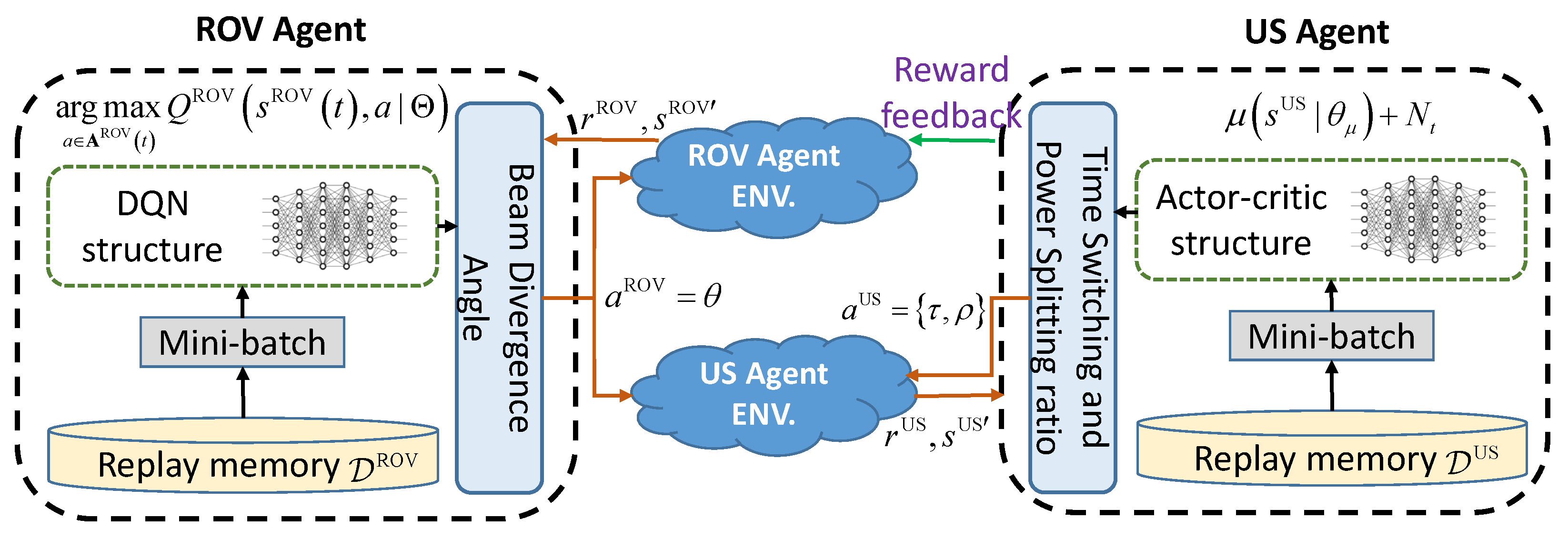
- To address the challenges of this communication scenario, we propose a hierarchical deep Q-network (DQN)–deep deterministic policy gradient (DDPG) algorithm. This algorithm involves two reinforcement learning (RL) agents: the ROV agent and the US agent. The role of the ROV agent is to determine the beam-divergence angle that maximizes the received optical power at the US node while ensuring a seamless optical link. On the other hand, the US agent, influenced by the decisions of the ROV agent, is responsible for determining the TS and PS ratios that maximize the EH without compromising the required communication performance.
- Through extensive simulations, we demonstrate that the proposed algorithm successfully maximizes the EH while maintaining the predetermined communication requirement at the US. The adaptive nature of the algorithm allows it to dynamically adjust the system parameters in response to changing underwater environmental conditions and sensor requirements, therefore enabling efficient and sustainable energy transfer and communication in underwater environments.
1.2. Organization
2. System Model
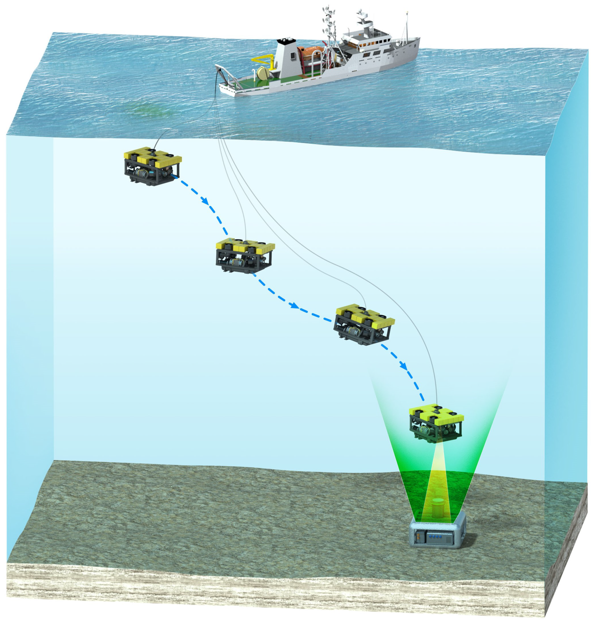
2.1. Network Model
- First, the ROV is launched into the ocean from the support vessel using a launch and recovery system (LARS). Once in the water, the ROV moves to the location where the US is located. At this location, the ROV performs SLIPT to not only transmit control data (e.g., wake-up or communication completion data) but also transfer power.
- Perceiving the control data and power, the US proceeds to transmit its collected sensing data to the ROV via LED-based UOWC. Although LED-based UOWC may have a relatively lower data rate compared to that of LD-based UOWC, it still provides a sufficient data rate (e.g., more than Mbps [23]) to transmit the sensing data with high reliability.
- Once the data reception process is complete, the ROV is retrieved and brought back to the support vessel for recovery, which is facilitated by the LARS.
2.2. Signal Model
2.3. Underwater Optical Channel Model
3. Underwater Hybrid Time Switching–Power Splitting (TS–PS) SLIPT
- In the first phase (referred to as EH mode), with a duration of , only EH is conducted (similar to the TS method). In this phase, there is no need to transfer information, such that DC bias can be set to its maximum value (i.e., ) to maximize EH, which leads to . The AC component in this phase is blocked by an inductor, such that only the DC component (i.e., ) passes through the EH block as illustrated in Figure 2.
- In the second phase (referred to as PS mode) with a duration of , the receiver conducts the PS method to perform EH and ID at the same time. For this, the received signal power is split into two streams using the power-splitting factor . As a result, and are dedicated for EH and ID, respectively. Through the suppression of the AC or DC component, the inputs to the EH and ID blocks can be presented as and , respectively, where is the AC–DC conversion efficiency [31], and is the average of the AC component.
3.1. Performance Metric 1: Energy Harvesting
3.2. Performance Metric 2: Spectral Efficiency
4. Proposed Algorithm
4.1. ROV Agent: Beam-Divergence Angle Adaptation
4.2. US Agent: SLIPT Adaptation
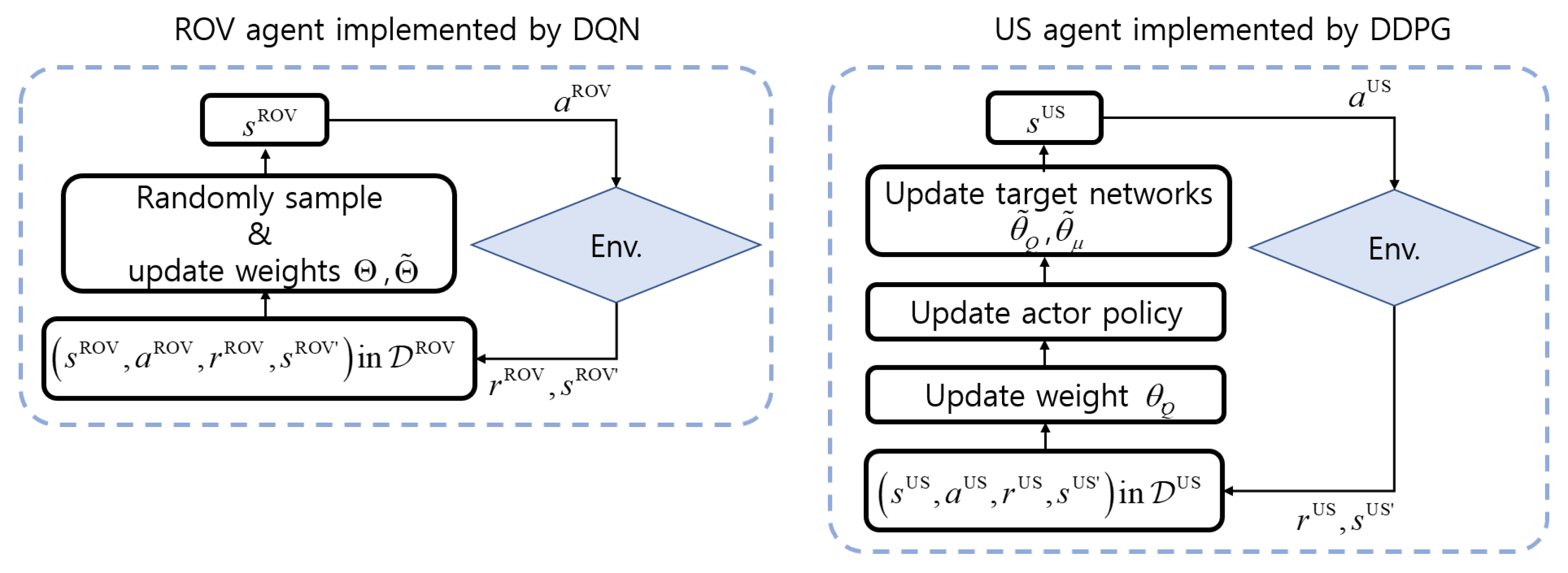
4.3. Proposed Algorithm
| Algorithm 1: DQN algorithm for determining the beam-divergence angle at the ROV agent. |
 |
| Algorithm 2: DDPG algorithm for determining TS and PS ratios at the US agent. |
 |
4.4. Verification for Online Operation via Computational Complexity Analysis
5. Simulation Results
5.1. Simulation Parameters
5.2. Benchmark Algorithms
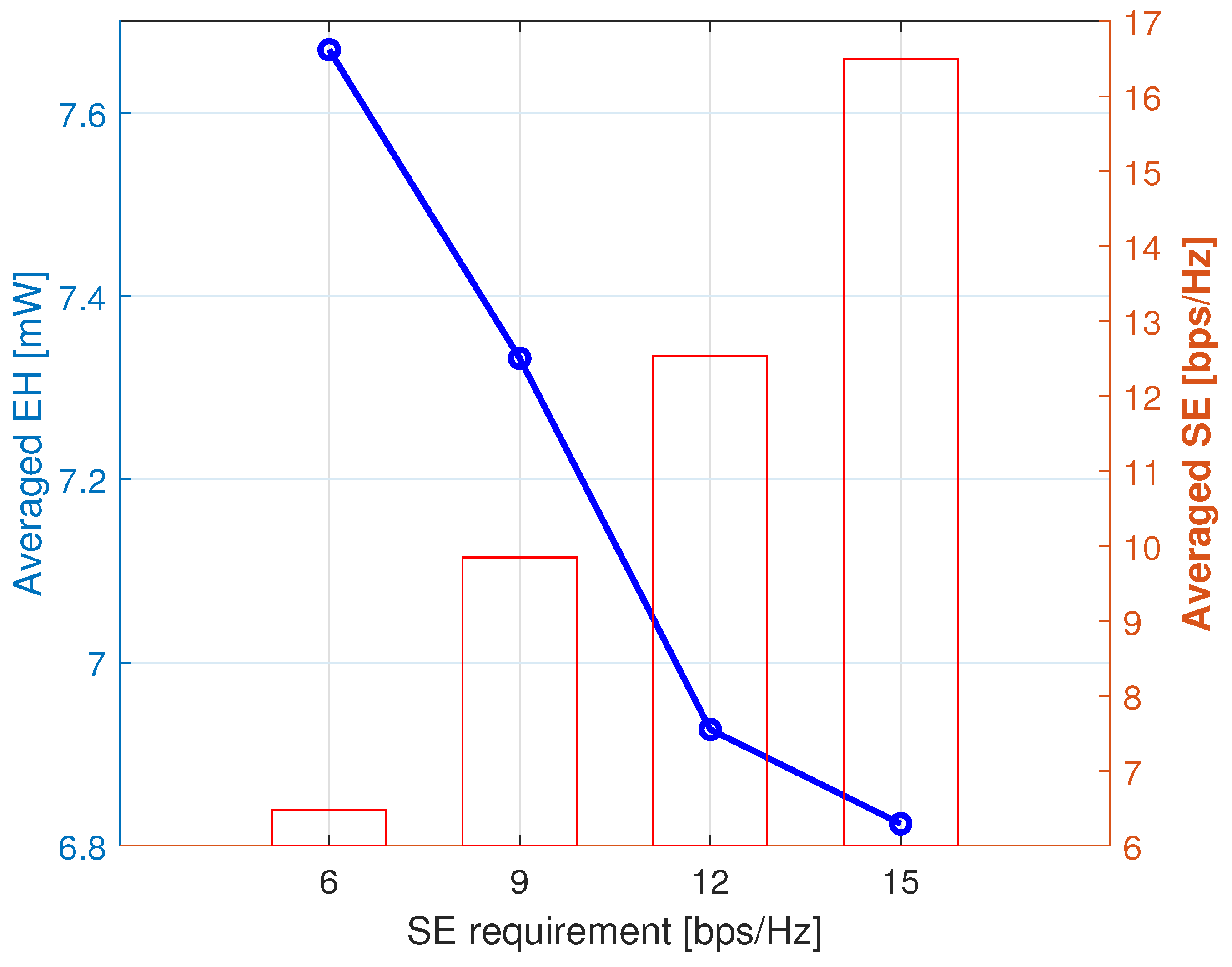
5.3. Simulation Results
6. Conclusions
Author Contributions
Funding
Institutional Review Board Statement
Informed Consent Statement
Data Availability Statement
Conflicts of Interest
Abbreviations
| UOWC | Underwater optical wireless communication |
| SLIPT | Simultaneous lightwave information and power transfer |
| SWIPT | Simultaneous wireless information and power transfer |
| TS | Time-switching |
| LD | Laser diode |
| EH | Energy harvesting |
| SE | Spectral efficiency |
| PS | Power splitting |
| ROV | Remotely operated vehicle |
| US | Underwater sensor |
| LED | Light-emitting diode |
| DQN | Deep Q-network |
| DDPG | Deep deterministic policy gradient |
| RL | Reinforcement learning |
| 3D | Three-dimensional |
| LARS | Launch and recovery system |
| IM/DD | Intensity modulation and direct detection |
| PAM | Pulse amplitude modulation |
| AWGN | Additive white Gaussian noise |
| BL | Beer-Lamber |
| LN | Log-normal |
| Probability density function | |
| ID | Information decoding |
| MPP | Maximum power point |
| SNR | Signal-to-noise ratio |
| MDP | Markov decision process |
| DNN | Deep neural network |
| MSE | Mean-squared error |
| DRL | Deep-reinforcement learning |
| ADS | AC–DC separation |
Glossary
| Explanation of Key Symbols | |||
| Symbols | Explanation | Symbols | Explanation |
| M | Modulation level | T | Time duration of data frame |
| Symbol interval | x | M-PAM symbol | |
| A | Peak amplitude | maximum input bias current | |
| minimum input bias current | Instantaneous emitted optical intensity signal | ||
| Slope efficiency of LD | B | DC bias | |
| Instantaneous received optical power | h | Underwater channel coefficient | |
| Attenuation loss | Geometrical loss | ||
| Fading | Received electrical signal | ||
| r | Solar panel responsivity | n | Additive white Gaussian noise |
| AC component of received signal | DC component of received signal | ||
| Inclination angle | d | Distance between ROV and US | |
| Attenuation coefficient | Absorption coefficient | ||
| Scattering coefficient | Aperture area | ||
| Beam-divergence angle | X | Log-amplitude coefficient | |
| Scintillation index | Time duration of EH | ||
| Time duration of ID | time-switching factor | ||
| power-splitting factor | AC-to-DC conversion efficiency | ||
| Maximum output power | Open circuit voltage | ||
| Thermal voltage | Dark saturation current | ||
| Indicator for use of AC component in EH | F | Fill factor | |
| optimal value of MPP voltage | optimal value of MPP current | ||
| Average electrical SNR | Noise power spectral density | ||
| Low bound of SE | State space of ROV | ||
| State space of US agent | Action space of ROV agent | ||
| Action space of US agent | Reward of ROV agent | ||
| Reward of US agent | Minimum beam-divergence angle | ||
| maximum beam-divergence angle | t | Time slot | |
| Historical information | l | Sliding window size | |
| Set of weights | Mean-squared error loss function | ||
| Experience replay buffer | Target value of ROV agent | ||
| Target value of US agent | discount factor |
References
- Kaushal, H.; Kaddoum, G. Underwater Optical Wireless Communication. IEEE Access 2016, 4, 1518–1547. [Google Scholar] [CrossRef]
- Schirripa Spagnolo, G.; Cozzella, L.; Leccese, F. Underwater Optical Wireless Communications: Overview. Sensors 2020, 20, 2261. [Google Scholar] [CrossRef] [PubMed]
- Shihada, B.; Amin, O.; Bainbridge, C.; Jardak, S.; Alkhazragi, O.; Ng, T.K.; Ooi, B.; Berumen, M.; Alouini, M.S. Aqua-Fi: Delivering Internet Underwater Using Wireless Optical Networks. IEEE Commun. Mag. 2020, 58, 84–89. [Google Scholar] [CrossRef]
- Johnson, L.J.; Green, R.J.; Leeson, M.S. Underwater optical wireless communications: Depth-dependent beam refraction. Appl. Opt. 2014, 53, 7273–7277. [Google Scholar] [CrossRef]
- Sahu, S.K.; Shanmugam, P. A study on the effect of scattering properties of marine particles on underwater optical wireless communication channel characteristics. In Proceedings of the OCEANS 2017, Aberdeen, Scotland, 19–22 June 2017; pp. 1–7. [Google Scholar]
- Elamassie, M.; Miramirkhani, F.; Uysal, M. Performance Characterization of Underwater Visible Light Communication. IEEE Trans. Commun. 2019, 67, 543–552. [Google Scholar] [CrossRef]
- Elamassie, M.; Uysal, M. Vertical Underwater Visible Light Communication Links: Channel Modeling and Performance Analysis. IEEE Trans. Wirel. Commun. 2020, 19, 6948–6959. [Google Scholar] [CrossRef]
- Gabriel, C.; Khalighi, M.A.; Bourennane, S.; Léon, P.; Rigaud, V. Misalignment considerations in point-to-point underwater wireless optical links. In Proceedings of the MTS/IEEE OCEANS, Bergen, Norway, 10–14 June 2013; pp. 1–5. [Google Scholar]
- Shin, H.; Kim, S.M.; Song, Y. Learning-Aided Joint Beam Divergence Angle and Power Optimization for Seamless and Energy-Efficient Underwater Optical Communication. IEEE Internet Things J. 2023, 10, 22726–22739. [Google Scholar] [CrossRef]
- Shin, H.; Baek, S.; Song, Y. Multidimensional Beam Optimization in Underwater Optical Wireless Communication Based on Deep Reinforcement Learning. IEEE Internet Things J. 2024, 11, 28623–28634. [Google Scholar] [CrossRef]
- Romdhane, I.; Kaddoum, G. A Reinforcement Learning based Beam Adaptation for Underwater Optical Wireless Communications. IEEE Internet Things J. 2022, 9, 20270–20281. [Google Scholar] [CrossRef]
- Guo, Y.; Xiong, K.; Gao, B.; Fan, P.; Ng, D.W.K.; Letaief, K.B. Max-Min Fairness in Rate-Splitting Multiple Access-Based VLC Networks With SLIPT. IEEE Internet Things J. 2024. [Google Scholar] [CrossRef]
- Zhang, R.; Xiong, K.; Lu, Y.; Ng, D.W.K.; Fan, P.; Letaief, K.B. SWIPT-Enabled Cell-Free Massive MIMO-NOMA Networks: A Machine Learning-Based Approach. IEEE Trans. Wirel. Commun. 2024, 23, 6701–6718. [Google Scholar] [CrossRef]
- Zhang, R.; Xiong, K.; Lu, Y.; Fan, P.; Ng, D.W.K.; Letaief, K.B. Energy Efficiency Maximization in RIS-Assisted SWIPT Networks with RSMA: A PPO-Based Approach. IEEE J. Sel. Areas Commun. 2023, 41, 1413–1430. [Google Scholar] [CrossRef]
- Filho, J.I.d.O.; Trichili, A.; Ooi, B.S.; Alouini, M.S.; Salama, K.N. Toward Self-Powered Internet of Underwater Things Devices. IEEE Commun. Mag. 2020, 58, 68–73. [Google Scholar] [CrossRef]
- Ammar, S.; Amin, O.; Alouini, M.S.; Shihada, B. Energy-Aware Underwater Optical System With Combined Solar Cell and SPAD Receiver. IEEE Commun. Lett. 2022, 26, 59–63. [Google Scholar] [CrossRef]
- Uysal, M.; Ghasvarianjahromi, S.; Karbalayghareh, M.; Diamantoulakis, P.D.; Karagiannidis, G.K.; Sait, S.M. SLIPT for Underwater Visible Light Communications: Performance Analysis and Optimization. IEEE Trans. Wirel. Commun. 2021, 20, 6715–6728. [Google Scholar] [CrossRef]
- Kogo, T.; Kozawa, Y.; Habuchi, H. Chlorophyll concentration-based CSK constellation point design for underwater SLIPT with priority on communication performance. In Proceedings of the International Symposium on Wireless Personal Multimedia Communications (WPMC), Okayama, Japan, 14–16 December 2021; pp. 1–6. [Google Scholar]
- Majlesein, B.; Guerra, V.; Rabadan, J.; Rufo, J.; Perez-Jimenez, R. Evaluation of Communication Link Performance and Charging Speed in Self-Powered Internet of Underwater Things Devices. IEEE Access 2022, 10, 100566–100575. [Google Scholar] [CrossRef]
- Ye, K.; Zou, C.; Yang, F. Dual-Hop Underwater Optical Wireless Communication System with Simultaneous Lightwave Information and Power Transfer. IEEE Photonics J. 2021, 13, 1–7. [Google Scholar] [CrossRef]
- Palitharathna, K.W.; Suraweera, H.A.; Godaliyadda, R.I.; Herath, V.R.; Ding, Z. Lightwave Power Transfer in Full-Duplex NOMA Underwater Optical Wireless Communication Systems. IEEE Commun. Lett. 2022, 26, 622–626. [Google Scholar] [CrossRef]
- Aguirre-Castro, O.A.; Inzunza-González, E.; García-Guerrero, E.E.; Tlelo-Cuautle, E.; López-Bonilla, O.R.; Olguín-Tiznado, J.E.; Cárdenas-Valdez, J.R. Design and Construction of an ROV for Underwater Exploration. Sensors 2019, 19, 5387. [Google Scholar] [CrossRef]
- Wei, W.; Zhang, C.; Zhang, W.; Jiang, W.; Shu, C.; Qiao, X. LED-Based Underwater Wireless Optical Communication for Small Mobile Platforms: Experimental Channel Study in Highly-Turbid Lake Water. IEEE Access 2020, 8, 169304–169313. [Google Scholar] [CrossRef]
- Mizukoshi, I.; Kazuhiko, N.; Hanawa, M. Underwater optical wireless transmission of 405nm, 968Mbit/s optical IM/DD-OFDM signals. In Proceedings of the OptoElectronics and Communication Conference and Australian Conference on Optical Fibre Technology, Melbourne, Australia, 6–10 July 2014; pp. 216–217. [Google Scholar]
- Dimitrov, S.; Sinanovic, S.; Haas, H. Signal Shaping and Modulation for Optical Wireless Communication. J. Lightw. Technol. 2012, 30, 1319–1328. [Google Scholar] [CrossRef]
- Mobley, C.D.; Gentili, B.; Gordon, H.R.; Jin, Z.; Kattawar, G.W.; Morel, A.; Reinersman, P.; Stamnes, K.; Stavn, R.H. Comparison of numerical models for computing underwater light fields. Appl. Opt. 1993, 32, 7484–7504. [Google Scholar] [CrossRef] [PubMed]
- Eroğlu, Y.S.; Yapıcı, Y.; Güvenç, I. Impact of Random Receiver Orientation on Visible Light Communications Channel. IEEE Trans. Commun. 2019, 67, 1313–1325. [Google Scholar] [CrossRef]
- Celik, A.; Saeed, N.; Shihada, B.; Al-Naffouri, T.Y.; Alouini, M.S. End-to-End Performance Analysis of Underwater Optical Wireless Relaying and Routing Techniques Under Location Uncertainty. IEEE Trans. Wirel. Commun. 2020, 19, 1167–1181. [Google Scholar] [CrossRef]
- Korotkova, O.; Farwell, N. Light scintillation in oceanic turbulence. Waves Random Complex Media 2012, 22, 260–266. [Google Scholar] [CrossRef]
- Navidpour, S.M.; Uysal, M.; Kavehrad, M. BER Performance of Free-Space Optical Transmission with Spatial Diversity. IEEE Trans. Wirel. Commun. 2007, 6, 2813–2819. [Google Scholar] [CrossRef]
- Sandalidis, H.G.; Vavoulas, A.; Tsiftsis, T.A.; Vaiopoulos, N. Illumination, data transmission, and energy harvesting: The threefold advantage of VLC. Appl. Opt. 2017, 56, 3421–3427. [Google Scholar] [CrossRef]
- Kyritsis, A.; Papanikolaou, N.; Tatakis, E.C. A novel Parallel Active Filter for Current Pulsation Smoothing on single stage grid-connected AC-PV modules. In Proceedings of the European Conference on Power Electronics and Applications, Aalborg, Denmark, 2–5 September 2007; pp. 1–10. [Google Scholar]
- Li, C.; Jia, W.; Tao, Q.; Sun, M. Solar cell phone charger performance in indoor environment. In Proceedings of the IEEE 37th Annual Northeast Bioengineering Conference (NEBEC), New York, NY, USA, 1–3 April 2011; pp. 1–2. [Google Scholar]
- Zainal, N.A.; Ajisman; Yusoff, A.R. Modelling of Photovoltaic Module Using Matlab Simulink. IOP Conf. Ser. Mater. Sci. Eng. 2016, 114, 012137. [Google Scholar] [CrossRef]
- Esram, T.; Chapman, P.L. Comparison of Photovoltaic Array Maximum Power Point Tracking Techniques. IEEE Trans. Energy Convers. 2007, 22, 439–449. [Google Scholar] [CrossRef]
- Wang, J.B.; Hu, Q.S.; Wang, J.; Chen, M.; Wang, J.Y. Tight Bounds on Channel Capacity for Dimmable Visible Light Communications. J. Light. Technol. 2013, 31, 3771–3779. [Google Scholar] [CrossRef]
- Mnih, V.; Kavukcuoglu, K.; Silver, D.; Rusu, A.A.; Veness, J.; Bellemare, M.G.; Graves, A.; Riedmiller, M.; Fidjeland, A.K.; Ostrovski, G.; et al. Human-level control through deep reinforcement learning. Nature 2015, 518, 529–533. [Google Scholar] [CrossRef] [PubMed]
- Lillicrap, T.P. Continuous control with deep reinforcement learning. In Proceedings of the International Conference on Learning Representations (ICLR), San Juan, PR, USA, 2–4 May 2016; pp. 1–14. [Google Scholar]
- Li, C.; Xia, J.; Liu, F.; Li, D.; Fan, L.; Karagiannidis, G.K.; Nallanathan, A. Dynamic Offloading for Multiuser Muti-CAP MEC Networks: A Deep Reinforcement Learning Approach. IEEE Trans. Veh. Technol. 2021, 70, 2922–2927. [Google Scholar] [CrossRef]
- Xu, K.; Shen, Z.; Wang, Y.; Xia, X.; Zhang, D. Hybrid Time-Switching and Power Splitting SWIPT for Full-Duplex Massive MIMO Systems: A Beam-Domain Approach. IEEE Trans. Veh. Technol. 2018, 67, 7257–7274. [Google Scholar] [CrossRef]
- Kim, S.M.; Won, J.S. Simultaneous reception of visible light communication and optical energy using a solar cell receiver. In Proceedings of the International Conference on ICT Convergence (ICTC), Jeju, Republic of Korea, 14–16 October 2013; pp. 896–897. [Google Scholar]
- Jalbert, J.; Baker, J.; Duchesney, J.; Pietryka, P.; Dalton, W.; Blidberg, D.R.; Chappell, S.; Nitzel, R.; Holappa, K. A solar-powered autonomous underwater vehicle. In Proceedings of the MTS/IEEE Oceans, San Diego, CA, USA, 22–26 September 2003; Volume 2, pp. 1132–1140. [Google Scholar]


| Parameter | Value |
|---|---|
| Time duration of a data frame T | 1 s |
| Distance between ROV and US | 10 m |
| Receiver Aperture diameter | 0.2 m |
| Extinction coefficient | 0.15 (clean ocean) |
| Solar panel responsibility r | 0.6 A/W |
| Slope efficiency of LD | 1.33 W/A |
| Maximum input bias current | 1.2 A |
| Minimum input bias current | 0.2 A |
| Fill factor F | 0.75 |
| Thermal voltage | 0.025 W |
| Dark saturation current | A |
| Noise power spectral density | W/Hz |
| Mean of inclination angle | 0.0436 rad |
| Standard deviation of inclination angle | 0.0087 rad |
| Hyperparameter | Agent |
|---|---|
| for -greedy | 0.01 |
| Mini-batch size | 64 |
| Optimizer | Adam |
| Activation function | Relu |
| Learning rate | |
| Experience replay buffer size | 2000 |
| Discount factor | 0.99 |
| Considered time slots for | 2 |
| Parameter | Value |
|---|---|
| Mini-batch size | 64 |
| Experience replay buffer size | |
| Discount factor | 0.99 |
| Learning rate of actor | |
| Learning rate of critic | 3 × |
| Soft update rate of target parameters | 2 × |
Disclaimer/Publisher’s Note: The statements, opinions and data contained in all publications are solely those of the individual author(s) and contributor(s) and not of MDPI and/or the editor(s). MDPI and/or the editor(s) disclaim responsibility for any injury to people or property resulting from any ideas, methods, instructions or products referred to in the content. |
© 2024 by the authors. Licensee MDPI, Basel, Switzerland. This article is an open access article distributed under the terms and conditions of the Creative Commons Attribution (CC BY) license (https://creativecommons.org/licenses/by/4.0/).
Share and Cite
Shin, H.; Jeong, S.; Baek, S.; Song, Y. Adaptive Control for Underwater Simultaneous Lightwave Information and Power Transfer: A Hierarchical Deep-Reinforcement Approach. J. Mar. Sci. Eng. 2024, 12, 1647. https://doi.org/10.3390/jmse12091647
Shin H, Jeong S, Baek S, Song Y. Adaptive Control for Underwater Simultaneous Lightwave Information and Power Transfer: A Hierarchical Deep-Reinforcement Approach. Journal of Marine Science and Engineering. 2024; 12(9):1647. https://doi.org/10.3390/jmse12091647
Chicago/Turabian StyleShin, Huicheol, Sangki Jeong, Seungjae Baek, and Yujae Song. 2024. "Adaptive Control for Underwater Simultaneous Lightwave Information and Power Transfer: A Hierarchical Deep-Reinforcement Approach" Journal of Marine Science and Engineering 12, no. 9: 1647. https://doi.org/10.3390/jmse12091647
APA StyleShin, H., Jeong, S., Baek, S., & Song, Y. (2024). Adaptive Control for Underwater Simultaneous Lightwave Information and Power Transfer: A Hierarchical Deep-Reinforcement Approach. Journal of Marine Science and Engineering, 12(9), 1647. https://doi.org/10.3390/jmse12091647