1. Introduction
Acoustic waves have much smaller absorption coefficients underwater than light and electromagnetic waves. Therefore, sonar equipment with acoustic waves acting as the carrier plays a very important role in marine monitoring, maritime military operations, and underwater search and rescue. Due to the particularity and complexity of the underwater environment, the echo signals received by sonar are inevitably affected by factors such as channel propagation loss, ocean noise, multipath effects, and reverberation, resulting in the existence of features in sonar images such as low resolution, blurred target edge, and significant speckle noise [
1,
2,
3]. In order to improve the visual effect of sonar images, denoising preprocessing technology has been widely used in feature extraction, target recognition, and image segmentation [
4]. Moreover, the application characteristics of sonar images mean that speckle noise is mainly caused by the sediment echo signals which are related to the background of seafloor sediment and can be obtained by prior modeling.
According to different processing domains, traditional image denoising algorithms can be generally divided into spatial domain filtering [
5] and transform domain filtering methods [
6]. The spatial domain filtering method is one of the earlier classical image denoising techniques and there is much current research. An adaptive median filtering algorithm based on quadratic detection of noise and neighborhood pixel restoration was used to improve the shortcomings of classical median filtering in [
7]. Lee, Kuan, Frost, and SRAD filtering are also categories of spatial domain filtering [
8,
9,
10]. The authors of [
11] introduced a new method based on the combination of three spatial domain filters. Although the spatial domain filtering method has achieved a certain denoising effect, there are certain drawbacks: the processed image is usually too smooth, and it can easily cause blurred edge and detail loss. However, the another transform domain filtering method contains common Discrete Cosine Transform (DCT) [
12], principal component analysis (PCA) [
13], and Wavelet denoising algorithms [
14]. Based on wavelet transform, a direction parameter was added and the Curvelet transform threshold filtering was used for noise removal [
15]. Researchers used the Curvelet method for sonar image denoising as well in [
16,
17]. The transform domain filtering method can achieve a certain denoising effect, but it will remove the high frequency components of the signal itself at the same time, which results in detail loss.
In addition, tensor-based methods have been also widely used in image denoising. A method based on the Tucker decomposition with automatically determined ranks of factoring tensors was proposed for speckle noise reduction in the side-scan sonar images [
18]. In [
19], a nonlocal low-rank regularized CANDECOMP/PARAFAC (CP) tensor decomposition (NLR-CPTD) was proposed to fully utilize these two intrinsic priors, which can greatly promote the denoising performance in various quality assessments. Researchers proposed a spatial-spectral TV regularized LR tensor factorization (SSTV-LRTF) method to remove mixed noise in HSIs [
20]. However, the research on tensor decomposition methods is mainly focused on hyperspectral images, and there have been still few researches on sonar image denoising.
In order to obtain a better denoising effect, deep learning-based denoising algorithms have become a research hotspot in the field of signal processing in recent years. DnCNNs were combined with learning algorithms and regularization methods for image denoising in [
21]. The authors of [
22] used the automatic encoder algorithm based on convolutional neural network to perform sonar image denoising. In [
23], a convolutional neural network based on a denoiser that could utilize the multi-scale redundancy of natural image was proposed. It is well known that deep learning can achieve better results than traditional methods. However, deep neural networks have the disadvantages of huge computation amount, slow training, time-consuming, and inconvenient storage. The required dataset is also very large. In particular, the purpose of denoising cannot be achieved when the training data is insufficient. Most importantly, it is not suitable for such applications due to the high calculation amount and the large requirement of original images considering that sonar is carried by AUV for capturing sonar images and performing calculation.
The dictionary learning-based denoising method is more suitable for sonar application scenarios and it is easier to model. Compared with deep learning methods, it can greatly reduce the calculation amount and more easily integrated into AUV systems. In addition, the dictionary learning method based on image sparse representation can effectively achieve denoising as well [
24]. In [
25], a novel supervised dictionary learning model with smooth shrinkage was proposed for image denoising. The uncertainty of estimation was considered and an adaptive Bayesian method was used to generate the sparse representation in [
26]. Moreover, a polarization image sensor denoising algorithm based on K-singular value decomposition (K-SVD) was proposed in [
27]. In summary, dictionary learning denoising method can increase the flexibility and adaptability for data processing. However, most of these methods are complicated and the performance should be improved.
In order to solve the above problems, for sonar speckle noise reduction, we propose a new adaptive dictionary learning method based on multi-resolution characteristics, which combine K-SVD dictionary learning with wavelet transform. The proposed method not only has the characteristics of dictionary learning, but also inherits the multi-resolution and local characteristics of wavelet analysis. Its advantage is the dictionary contains atoms at different resolution scales, which can represent the original image more effectively. Experiment results show that the proposed method has better ability for speckle noise reduction and edge detail preservation. At the same time, the calculation time is greatly reduced and the efficiency is significantly improved.
This paper is organized as follows. In
Section 2, we introduce the statistical model of sonar imaging speckle noise. The proposed method and the principle of dictionary learning-based denoising are described in
Section 3. The experiments and results are discussed in
Section 4.
Section 5 gives the conclusion.
2. Statistical Model of Sonar Imaging
2.1. Sonar Imaging Principle
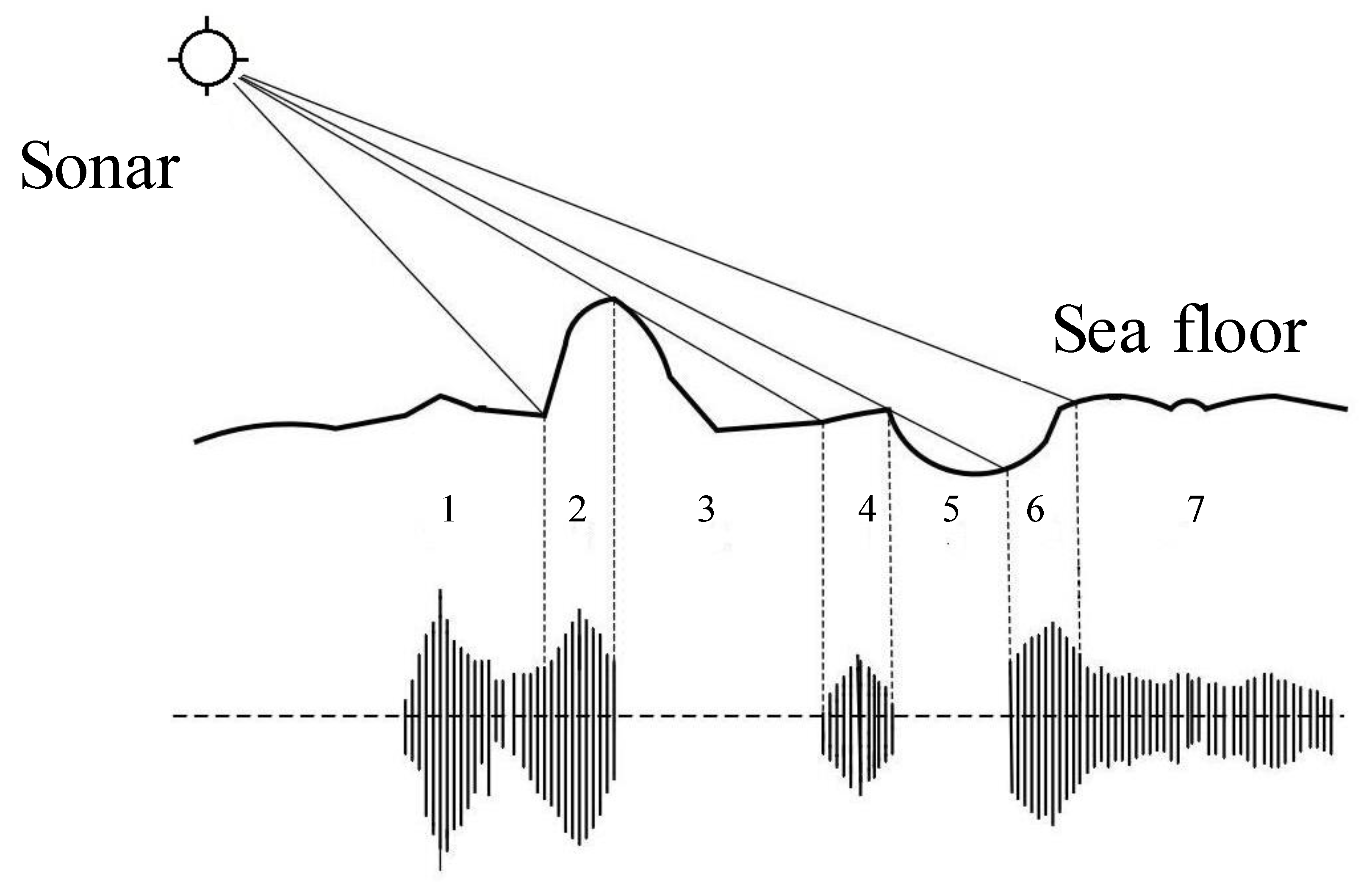
In most sonar imaging systems, the sonar device actively emits acoustic waves that will be reflected when touching target or seafloor, and the echo is received by transducer. As shown in
Figure 1, the pixel coordinates correspond to the arrival time of echo, and the gray pixel values correspond to the echo intensity. Specifically, the strong part of the received echo corresponds to the target, which is indicated in the white area of image; the black area corresponds to the weaker echo region. The remaining area consists of background noise, mostly from the background reflections of seafloor sediment. It is characterized by alternating very small bright and dark areas [
28]. Finally, each received echo data is sequentially arranged, and a 2-D sonar image can be obtained.
2.2. Speckle Noise Model of Sonar Image
Researches show that reverberation is the primary background interference of active sonar systems, which is the sum of received scattered waves reflecting on the seawater boundary and scatting on seawater volume. The echoes among different scatterers cancel each other out or reinforce each other, resulting in the occurrence of fluctuations in the amplitudes of echoes. This phenomenon appears as a grainy black and white texture on the sonar image, which is known as speckle noise.
According to the submarine reverberation model mentioned in [
29], it is assumed that the signal emitted by acoustic source is
and the reverberation at time
t is expressed as
where
N represents the sum of all scattering elements contributing to time
t,
is the number of scatterers (the value is 0 or 1) at
in each scattering element
,
is the attenuation factor of scattered waves in the two-way propagation,
is the scattering coefficient,
is the arrival time of echo,
is the center frequency of transmitted signal, and
represents the phase of scattering coefficient
. Besides,
,
, and
are independent of each other.
Suppose that
and
represent the instantaneous amplitude and phase value of the
scatterer, respectively, therefore
The real and imaginary parts of
can be obtained:
From the central limit theorem, we know that when N is large enough, and are both random variables which are subject to Gaussian random distribution. For random scatterers, and , which are in a uniform distribution from 0 to 2, are independent random variables. It can be seen that and are obedient to Gaussian random distribution; they are independent of each other, the mean value is zero, and the variance is same. Furthermore, the reverberation amplitude is a random variable following Rayleigh distribution. Therefore, it can be concluded that the envelope amplitude of reverberation follows Rayleigh distribution and its phase obeys uniform distribution.
The probability density function of amplitude is as follows.
represents the attenuation parameter of Rayleigh distribution.
2.3. Speckle Noise Simulation for Sonar Images
From the above analysis, it can be seen that a large number of scatterers make the value of each pixel fluctuate randomly, forming a granular speckle noise. Moreover, the probability density function of its amplitude obeys Rayleigh distribution. Therefore, the multiplicative noise model of speckle noise can be obtained:
where
x represents the expected true amplitude.
n and
y are random variables with the same distribution, which both obey translational Rayleigh distribution. The mean value of
n is 1.
If considering complicated underwater environment, the impact of environmental noise should be added. However, compared with multiplicative speckle noise, the effect of additive Gaussian noise is much smaller. In order to simplify the model, we ignore the influence of additive noise in this paper. Therefore, the speckle noise in sonar image can be roughly regarded as a multiplication process [
30].
Considering that the imaging mechanisms of sonar and ultrasound are similar, the Pizurica method for adding speckle noise to ultrasound images [
31] can also be used to simulate the speckle noise for sonar images. The method can simulate characteristics of speckle noise well. The specific steps are as follows.
Step 1 First, generate a complex Gaussian random field. The imaginary and real parts are both independent distribution of Gaussian random variables with the same mean value being 1 and same standard deviation. It is noted that the variance determines different level of speckle noise.
Step 2 Considering the neighborhood correlation of speckle noise, a low-pass average filtering of window is performed on the random field. Take out the amplitude of filtered output. Finally, multiply it with the reference image to obtain the simulated sonar image with speckle noise.
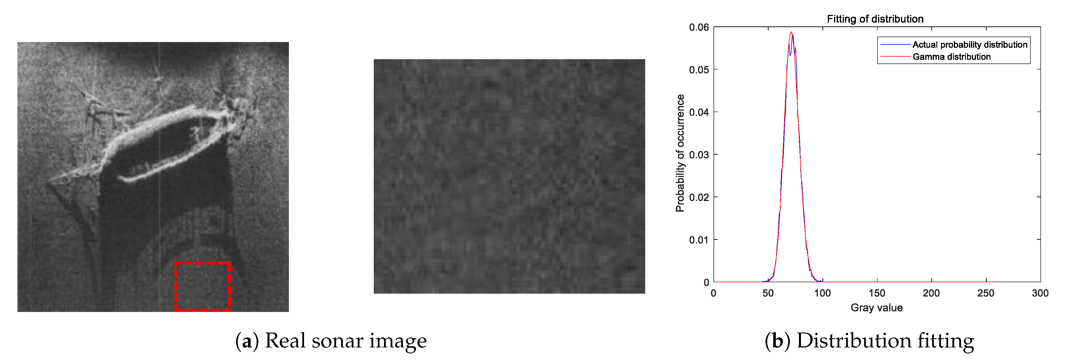
It is proved that there is an optimal structure for fitting the grayscale distribution of sonar image by using Gamma distribution [
32].
Figure 2 shows fitting results of the background grayscale probability distribution of real sonar image and Gamma distribution, where the fitting area is the red box in the image. It can be seen that the background grayscale distribution of the original sonar image can be fitted accurately by using Gamma statistical distribution. Similarly,
Figure 3 shows the fitting results of the simulated sonar image. Results show that using Gamma statistical distribution can accurately fit the gray distribution of the background area for the simulated noisy image. Therefore, the above speckle noise addition method can simulate the speckle noise of sonar image at an acceptable level. In this paper, we use the above method to add speckle noise to sonar image, and then use the generated noisy images for subsequent dictionary training and experimental verification.
It should be noted that the general denoising method is mainly used to deal with the additive noise model. In order to be able to use these existing algorithms, the above multiplicative noise model must to be transformed to a simple form. We take the logarithm of both sides of Equation (7) to obtain a sonar image containing approximately Gaussian additive noise. After logarithmic transformation, the probability density function of random variable
becomes
The density function defined by the above formula is called a double exponential or Fisher–Tippet density function. The mean and variance can be calculated by
where
is Digamma function, defined as
is the first-order Polygamma function. The m-order Polygamma function is defined as
The work in [
33] proved that Fisher–Tippet distribution of Rayleigh multiplicative noise after logarithmic transformation is approximately in line with additive Gaussian random noise, except for a small amount of large values. Therefore, denoising methods for additive Gaussian noise can be used for sonar images. Approximate additive Gaussian noise is obtained after logarithmic transformation. We then use similar Gaussian denoising methods to remove the speckle noise from sonar images, and finally perform logarithmic inverse transform to obtain the denoised image.
3. Proposed Denoising Algorithm
3.1. Sparse Representation for Sonar Image
Most of the information and energy of an image are concentrated on the coefficients with larger values. Therefore, we consider representing the image by a linear combination of the atoms in a dictionary. Sonar images also have inherent sparse structural characteristics [
34], and the distinction between useful information and noise in an image is determined by whether it is a sparse component of the image.
For an image, we consider a small image block
x size of
, and arrange it as a
n-dimension column vector
. Assume a redundant dictionary
, where
. The following model can be obtained.
is the number of nonzero elements in the coefficient , where . The solution of the above equation is sparse, and the basic idea is that each signal can be represented by a linear combination of some atoms in the redundant dictionary D.
In order to facilitate calculation, we use error constraint to replace . At the same time, define the sparse degree L, which meets . Actually, the number of dictionary atoms in the form of a linear combination to represent image block x does not exceed L. We use , which represents the above model.
In this paper, the speckle noise in sonar images can be roughly regarded as a multiplication process. To use the existing algorithms based on the additive noise model, the multiplicative noise model must be transformed to a simple form. We take the logarithm of both sides of the multiplication model to obtain a sonar image containing approximately additive Gaussian noise. Therefore, denoising methods for additive Gaussian noise can be used for sonar images. Approximate additive Gaussian noise is obtained after logarithmic transformation, then we use similar additive Gaussian denoising methods to remove speckle noise from sonar images, and finally perform logarithmic inverse transform to obtain the denoised image. Suppose
x is a signal that satisfies model
and
n is a Gaussian white noise signal with the mean value 0 and standard deviation
. There is a noisy signal
y based on approximate additive noise model after logarithmic transformation:
According to the Maximum Posteriori estimation (MAP), we can create the following model,
where
T depends on the values of
and
.
The denoised image is calculated by . Because there is a sparse representation of noise-free image under appropriate dictionary and the noise destroys sparsity of image information. The above model restores the original image by estimating sparse coefficients of the noise-free image so that noise can be removed.
If we translate the constraint of the above formula into a penalty item, we can get the model as follows,
where
is a penalty factor. Given an appropriate value
, the above two questions are consistent. The later discussion of this paper is based on model (16).
This problem is equivalent to minimizing the number of nonzero elements, that is, using as few atoms as possible to represent the image.
is the approximate error of this process. In general, the above problem is difficult to solve. We mainly use Orthogonal Matching Pursuit (OMP) [
35] to solve the problem in this paper.
3.2. Dictionary Learning and Updating
In this paper, we use the K-SVD framework for dictionary learning and updating [
27]. Noisy sonar images are used for training to construct an adaptive dictionary. Because K-SVD has the ability to suppress noise during the learning process, samples used for training can also be selected from noisy images. For a larger image
X size of
, we divide the image first and then rebuild the results. In order to prevent the occurrence of manually processing traces, the results of overlapping blocks can be averaged.
Assume that each block of the image belongs to sparse model
and
D is an unknown parameter. This problem can be modeled as follows,
where the first term is a log-likelihood global constraint, representing the degree of approximation between image
Y and its reconstructed image
X. The second and third terms are image priors, which guarantee that each block
has a sparse representation of bounded error at each position.
is a matrix block size of
extracted from the position
. Moreover, the coefficients
must be independent in order to satisfy the constraint form
.
First, dictionaries
D and
X are assumed to be fixed, and
can be calculated by OMP sparse decomposition method. Then, the dictionary is updated by K-SVD. After dictionary updating, we repeat the stage of sparse decomposition and update the dictionary continuously. These two steps are iterated until the algorithm converges or satisfies the predefined stop criterion. Finally, we can get sparse representation coefficients and a suitable dictionary. The output image can be calculated by using the updated dictionary and sparse coefficient matrix. The process of dictionary construction and updating is as Algorithm 1 [
34].
| Algorithm 1 Dictionary learning-based denoising algorithm |
- 1:
Input: noisy images - 2:
Output: denoised images - 3:
Begin - 4:
Initialization: , , , , D is redundant DCT dictionary - 5:
For j times - 6:
Do - 7:
Use OMP to approximate ; Calculate sparse representation vector of each block - 8:
For each column in D, find the set of these atoms ; Index in , calculate representation error: - 9:
Assume the column vector of matrix is ; Use SVD to decompose it: - 10:
Select the first column of U to update column of the dictionary; Use to update coefficient value - 11:
For all the columns of dictionary, repeat the above process to get a new dictionary and sparse representation coefficients. - 12:
End - 13:
Give all of the , fix these coefficients to update X; obtain: - 14:
Calculate the denoised image: Where I is a unit matrix and is a diagonal matrix. - 15:
End
|
where
j is the number of iterations.
and
C are parameters.
is the standard deviation of Gaussian white noise signal
y.
X is the noisy image, and
Y is the reconstructed image.
It should be noted that K-SVD can adaptively update the atoms in dictionary. K-SVD includes two steps: sparse decomposition and dictionary updating. The biggest difference between K-SVD and other algorithms is the dictionary updating process. K-SVD only updates one atom at a time; until all atoms in the dictionaries are updated, repeat the above process several times to get the representation coefficient of signal and a dictionary after training.
After sparse decomposition, the atom needs to be updated to get a better dictionary. In this stage, dictionary D updates one column each time, and fixes other columns in the dictionary. is the column in the dictionary. is the index of signal atom . Through decomposing by using Singular Value Decomposition (SVD), we can get . The column of the dictionary is updated with the first column of U, and the coefficient is updated by . Repeat this process for all columns in the dictionary (hence named K-SVD). After dictionary updating, the sparse decomposition stage is repeated, and the dictionary is updated again. These two steps are iteratively performed until the algorithm converges or meets the predefined stopping criterion, and finally the sparse representation coefficient and a suitable dictionary are obtained.
3.3. Proposed Solution for Dictionary Training
Based on the adaptive dictionary constructed by K-SVD in the previous section, we propose a new method for dictionary training in this section. On the framework of K-SVD, we combine multi-resolution and local characteristics of wavelets to obtain a learning dictionary with structural information at different scales (multi-resolution adaptive dictionary). This constructed dictionary contains atoms at different resolution scales, where the large-scale atoms can effectively describe the overall structure of image and the small-scale atoms can capture the small features. Therefore, the newly constructed dictionary can effectively represent original image.
Multi-resolution analysis can be visually represented by using a set of nested multi-resolution subspaces. It is assumed that the frequency space of original signal is expressed as
, which is decomposed into two subspaces of low frequency
and high frequency
, and then
is subdivided into low-frequency components
and high-frequency components
, and so on. The following characteristics of subspace can be obtained,
where ⊕ means the orthogonal sum of two subspaces;
represents the subspace corresponding to resolution
; the space vector
formed by the expansion and translation of wavelet function is the orthogonal complement space of
;
reflects the high frequency subspace of the spatial signal details of
;
shows the low frequency subspace of the spatial signal profile of
. Moreover, the model’s physical meaning is that a space
with resolution
can be approximated by finite subspaces.
As the image is a two-dimensional signal which is similar to the multi-resolution analysis of a one-dimensional signal, we need to perform corresponding expansion and translate the space into , where the one-dimensional scale function becomes .
Assuming
is the multi-resolution analysis of space
, there is a tensor space
, where
constitutes the multi-resolution analysis of space
and the two-dimensional scale function of multi-resolution analysis
is
where
is the one-dimensional scale function of
. For each
, the normative orthogonal basis of
consists of function systems
. Moreover,
is called separable multi-resolution analysis of
. Because
and
are both low-pass scale functions,
is a smooth low-pass space.
If
represents the orthogonal wavelet basis of one-dimensional multi-resolution analysis
, the integer translation sequences of three wavelet functions of two-dimensional multi-resolution analysis is expressed as
Noted that the superscripts in the equation are not exponents, just index terms, which form the normalized orthogonal basis of
. Moreover, these three orthogonal basis reflecting the detailed information of the two-dimensional signal are band-pass. Specifically,
corresponds to the horizontal, vertical, and diagonal directions of the two-dimensional signal, respectively. For any arbitrary
at resolution of
, there are
The above equation indicates that the image is decomposed into sub-bands of these four directions: , , , and at resolution of , where represents the approximate components of image (the low frequency portion of image), and indicates the high frequency components or detail part at each direction. Specifically, corresponds to the high frequency component of vertical direction, belongs to the horizontal high frequency component and corresponds to the diagonal.
We propose an adaptive dictionary learning method with multi-resolution characteristics by combining K-SVD with wavelet transform. The proposed method not only has the characteristics of dictionary learning, but also inherits the multi-resolution and local characteristics of wavelet analysis. The advantage is the dictionary contains atoms at different resolution scales. The large-scale atoms can effectively describe the overall structure of image and the small-scale atoms can capture the small features. Therefore, the newly constructed dictionary can effectively represent original image. Our proposed method has better ability for speckle noise reduction and edge detail preservation. At the same time, the calculation time is greatly reduced and the efficiency is significantly improved. Algorithm 2 shows the proposed method.
| Algorithm 2 The proposed denoising algorithm |
- 1:
Input: noisy images - 2:
Output: denoised images - 3:
Begin - 4:
Perform 3-layers wavelet transform on the noisy sonar images - 5:
Extract the low-frequency coefficients of the first scale, and the high-frequency coefficients of each scale to train dictionaries respectively in steps: 6–15 - 6:
Initialization - 7:
Fix dictionary D and X in sparse model - 8:
For times - 9:
Do - 10:
Use OMP to calculate the sparse representation vector - 11:
Update the dictionary by K-SVD - 12:
Repeat the above steps to update dictionary and coefficient value by column - 13:
End - 14:
Obtain the newly constructed multiple adaptive dictionary and coefficient of sparse representation - 15:
Give all of the sparse coefficients, fix these coefficients to update X - 16:
Cascade these dictionaries to get the final multi-resolution adaptive dictionary - 17:
Perform logarithmic transform of the simulated noisy sonar image to transform multiplicative Rayleigh noise into approximate additive Gaussian noise - 18:
Decompose and reconstitute the image by using the above dictionaries - 19:
Calculate the denoised image - 20:
Perform inverse logarithmic transform for the denoised image - 21:
Obtain the final denoised image. - 22:
End
|
4. Experiments and Discussions
The denoising results of sonar images are given in this section, including the simulated noisy sonar images and the real sonar images. All the simulation results are obtained in the configuration of Pentium dual-core CPU, dominant frequency at 3.2GHz, 8G memory, Windows XP 32-bit operating system and MATLAB R2010b.
4.1. Denoising Results of Simulated Noisy Image
Above all, select the noise-free image as original image, and then add speckle noise of different levels to the image. The simulation method of speckle noise is mentioned in
Section 2. We use the proposed denoising method for simulated noisy sonar image, and compare it with several methods. The denoising comparison algorithms used in this paper include Lee filter [
36], Kuan filter [
37], Frost filter [
38], SRAD filter [
39], Wavelet-based denoising method [
14], Curvelet-based denoising method [
15], DCT-based denoising method [
12], and K-SVD denoising method [
34].
Figure 4 shows the original image and simulated noisy image.
Figure 5 shows the denoising results of different algorithms for the simulated image. The standard deviation of speckle noise is 0.9. It can be seen that the edge details are lost and there is still residual noise of spatial domain filtering methods such as Lee, Kuan, Frost, and SRAD. The Wavelet denoising retains edges well, but a lot of noise remains. Curvelet has a good effect on edge retention, but scratches exist. The K-SVD algorithm achieves better noise removal and edge retention. However, the performance of the proposed method is still the best in all respects. In addition, the proposed algorithm is far superior to K-SVD in terms of calculation efficiency. When
, K-SVD took 1270.11 seconds, and the proposed took 550.10 s. When
, K-SVD took 267.68 seconds, and the proposed took 169.39 seconds. When
, K-SVD took 315.76 seconds, and the proposed took 146.81 seconds. Therefore, the time efficiency of the proposed algorithm is nearly double that of K-SVD.
In addition, we use the full reference indicators for objective quality evaluation, including structural similarity index measurement (SSIM) and equivalent numbers of looks (ENL). SSIM evaluates image quality by comparing the structural characteristics of the original image and the distorted image, without error merging. The theoretical basis of this method is that natural images are based on texture characteristics. Pixels that are especially adjacent in space have strong correlations, and these correlations carry a lot of important image information. SSIM measures image similarity from three aspects: brightness, contrast, and structure. The larger the value, the better the algorithm. The goal of speckle noise suppression is to effectively suppress speckles while keeping the structural information in the image scene as much as possible. Therefore, ENL is introduced in this paper to measure the smoothness of uniform area, which can be used to measure the relative intensity of speckle noise in an image. It is also an index to measure the filtering performance of a filter. In the texture area, the smaller the ENL value, the better the texture information is maintained. In the uniform area, the larger the ENL value, the better the filtering effect.
Table 1,
Table 2 and
Table 3 show the values of the objective evaluation indexes of different algorithms when the standard deviation of noise is 0.3, 0.6, and 0.9, respectively. Each data in the table is a value obtained by averaging 10 simulation experiments. It can be seen that the performance of the proposed method is better than others by comparing the values of SSIM and ENL.
Figure 6a shows the values of objective evaluation index SSIM after filtering by various algorithms under different noise levels. Under the same noise pollution level, the proposed method has the highest SSIM value, which indicates that our method is better at removing speckle noise and preserves the image structure information well.
Figure 6b shows the ENL values under different noise levels. As can be seen from the graph, the proposed method has higher equivalent visual value, which means its speckle suppression effect is better.
4.2. Denoising Results of Real Sonar Images
The experiment images are selected from the side scan sonar image library
Fenn Enterprises on the website:
http://www.fennent.com/sonar.html. First, we grayscale the images and adjust the size to
. As there is no reference image, subjective observation method is selected to illustrate the denoising results of various algorithms. The three side scan sonar images are selected from the image library
Fenn Enterprises of size
.
It can be seen that the three original images contain speckle noise with different levels.
Figure 7,
Figure 8,
Figure 9 and
Figure 10 correspondingly show the denoising results. The denoising effect of the different methods has consistent characteristics on these three images and the results are consistent with the simulated noisy image. As can be seen from the figures, the traditional methods such as Lee, Kuan, Frost, Wavelet, and Curvelet have more residual noise. Moreover, SRAD appears visual blurring. Predictably, the proposed method achieves better results in suppressing speckle noise and detail retention than several other methods.


