Abstract
When waves propagate in coastal areas at depths lower than one half the wavelength, they exhibit a different signature at the sea surface and the observed wavelength pattern enables inferring bathymetries. Commonly, a spectral analysis using the fast Fourier transform (FFT) is employed to derive wavelength and wave direction of swell waves, in nearshore regions. Nevertheless, it is recognized that this method presents limitations, particularly regarding depth inversion limits that do not allow obtaining bathymetric data close to the shoreline. This work explores a wavelet spectral analysis to obtain bathymetric data. This new imaging methodology is applied over different seafloors with 2D and 3D features such as longshore bars or headlands. The synthetic images of the water surface are generated from a numerical Boussinesq-type model that simulates the propagation of both regular and irregular waves. The spectral analysis is carried to estimate the water depths, which are validated with the model’s bathymetry. Wavelet image processing methodology shows very positive results, revealing the capabilities of this new methodology to map shallow marine environments.
1. Introduction
The nearshore area is an extremely dynamic system, with variations in its morphology over short periods of time. Due to these rapid variations, constantly monitoring the morphology of the seafloor, especially in coastal and harbor areas, is particularly relevant for navigation safety and in terms of coastal erosion management. Currently, the most used methods for monitoring the seafloor are based on acoustic systems (e.g., single and multibeam echosounder). These methods, although presenting a very high precision, are relatively expensive and difficult to operate in shallow waters, and their use depends on favorable weather and wave conditions [1], so monitoring is not done regularly. In areas closer to the coast, the disadvantages mentioned above can be overcome with the use of satellite images obtained by remote sensing, which make use of various passive (e.g., SPOT, LandSat-8/OLI, etc.) and active sensors (e.g., TerraSAR-X, Sentinel-1, etc.). Better satellite image resolution is now available, which is particularly useful to obtain relatively high precision data. Additionally, satellite images allow monitoring the water depth, covering large and remote areas, where the seafloor topography can change relatively fast due to storms [2,3,4].
When waves propagate in coastal areas at depths lower than one half the wavelength, they exhibit specific sea surface features. Their shapes are controlled by the seafloor surface due to the interaction of the orbital wave motion with the bottom. Waves also leave their imprint on the seafloor in many ways, acting as sculptors on the ocean floor at different length scales (e.g., ripples and submerged coastal bars). This complex feedback system, due to the interplay between sediment transport and water motion, reflects a pattern at the sea surface that can be captured in satellite images. This enables inferring time-varying bathymetries, typical of shallow sandy coasts [5,6].
When wind-generated waves travel from open sea to coastal areas, the wave profile becomes less irregular, giving rise to a train of more regular long waves, moving in their own direction, categorized as swell [7]. In intermediate and shallow waters, the waves are slowed down and the swell wave’s pattern evidence changes in the wavelength. In physical terms, it is recognized that the approximation of waves to shallow areas, resulting in a decrease in the wavelength, is inextricably linked to water depths. In this way, it is possible to estimate bathymetry based on the detection of the wavelength variation.
Depth inversion methods using waves have an offshore depth limit which is associated to when the orbital wave motion no longer “feels” the bottom. This is exclusively a function of the waves’ wavelength and inversion can be undertaken in nearshore regions [8].
Satellite imagery contains information on the sea surface roughness which can be used to infer the waves’ wavelength [9]. Image processing plays a crucial role to quantify the wavelength changes. Spectral analysis emerges as a tool to support our understanding and to characterize the behavior of the wind-generated waves. In the aim of the context herein presented, the fast Fourier transform (FFT) spectral analysis is often used, being particularly suited to derive wavelength and wave direction of swell waves, in nearshore regions [10,11]. Although this methodology is a very commonly used tool and efficient numerical algorithms have been developed based on Fourier analysis, it is also recognized that this methodology presents limitations [12]. It is confined to the inner continental shelf for water depths between 15 and 30 m and, among other factors, part of the observed discrepancies between estimated FFT and observed bathymetry may be attributed to the selection of cell size, cell shift, and mode of implementation.
To overcome the FFT limitations, a new methodology based on the wavelet theory is proposed in this paper. The uses of wavelets have been successfully applied to various types of synthetic or field signals evidencing their potential [13,14,15]. The greatest advantage of the wavelet spectral methodology is that it enables computing the instantaneous frequency of the signals, also enabling the analysis of nonlinear and nonstationary signals, which are often present during wave propagation in intermediate and shallow waters [16,17].
This study makes use of the wavelet spectral methodology to estimate the wavelength variation along wave propagation. This new imaging methodology is explored over different seafloors with 2D and 3D features such as longshore bars or headlands. The surface wave field is simulated with a numerical Boussinesq-type model, forced with both regular and irregular waves, with the objective to replicate the wave wavelengths as observed in satellite images. Therefore, the estimated depths can be validated with the real bathymetry, assessing the capabilities of this methodology for the mapping of shallow marine bathymetry over broad areas.
2. Methodology
2.1. Depth Estimation
Remote sensing techniques have been employed by many researchers to obtain bathymetric information in coastal and estuarine environments [10,18,19]. The availability of high spatial resolution satellite images revolutionized the possibility to develop bathymetric models from the information of ocean waves propagating towards the coastal line. The changes in the sea surface evidenced by the swell wave’s pattern in the nearshore, based on its roughness and height, are directly linked with the local bathymetry.
For example, Synthetic Aperture Radar (SAR) satellite images provide a synoptic view of the wave field and have been used for the detection of the swell wave’s pattern to retrieve bathymetric data [10,12]. As the waves progress from deep to shallow waters, the images should show a pattern of nearly regularly spaced wave crests and troughs. The lighter tones (almost white) correspond to wave crests and the darker grey tones refer to wave troughs, enabling detection of the wavelength variation along the wave propagation.
Nearshore depths can be estimated from swell wavelength observations since the wavelength can be mathematically connected with local depth via the dispersion relation of Airy’s wave theory. This theory is an analytical solution of the momentum and mass conservation equations that describes the wave velocity field and pressure along the water column, and establishes a relation between the wave celerity, the frequency, and the water depth (linear dispersion relation). Using the linear dispersion relation, the approach taken to determine the depth of the ocean seafloor (h) meets the set of values of the local wavelength (L) and the wavelength at deep waters (L0):
Here, L0 is calculated from the wave period (T):
where g is the gravitational acceleration.
Local wavelengths are obtained from the horizontal and vertical components of the wavelength observed in the images, according to the methodology presented by [20]. Accordingly, the image is analyzed through rows and columns, providing the horizontal and vertical components of the wavelength between wave crests (Lx and Ly) and the wavelength is computed from the knowledge of both components:
2.2. Wavelets vs. FFT
Commonly, FFT is used for the computations of directional wave spectra from passive and active satellite images to retrieve the wavelength and wave direction, and to estimate the water depth by solving the linear dispersion relation (e.g., [10,11,12,21,22,23]). This methodology considers a 2D subimage, also referred to as a cell, that needs to resolve a sufficient number of waves in order to compute the FFT accurately.
The Fourier transform is used to decompose space-varying pixels, resulting in a two-dimensional frequency-domain representation of the information content in each cell. In the first step, a grid of points is defined over the image. The depth is estimated at each grid point from the knowledge of the dominant wavelength at the cell centered at that point. The computation is made from open sea to the shoreline, resulting in the bathymetric information for the target area.
As mentioned by Pereira et al. [12], the partitioning of the image into cells and the application of the FFT to each of the cells should consider a proper selection of the width of the cell. Each cell needs to contain sufficient information regarding the local wave characteristics to allow a proper identification of the dominant wave behavior in that region, but it cannot cover too vast a region since the waves might already present distinct characteristics through that cell.
Pereira et al. [12] investigated the repeatability of the FFT methodology in retrieving the nearshore bathymetry, using a set of four high temporal resolution images from Sentinel-1A with C-band SAR images. The results show that a combined solution that merges the results of all the image sets lightly improves the results obtained from each image. The application of this methodology is confined to the continental shelf for water depths between 15 and 30 m and the relative error of the water depth ranges between 6% and 10%, increasing errors for higher water depths. Among other factors, the authors attribute part of the discrepancies to the methodological FFT approach, regarding the selection of cell size, cell shift, and mode of implementation.
Although one recognizes the Fourier transform as a powerful tool in the signal processing field, it possesses some limitations. The Fourier transform re-expresses a function in terms of sinusoidal basis functions, that is, as a sum of sines and cosines functions with specific amplitudes and phases. It can be defined as frequency–amplitude decomposition, in that it has only frequency resolution and no time resolution. Therefore, we might be able to determine the frequencies (wavelength) present in a signal, but we do not know how they change in time (space).
In the past decades, the wavelet transform or wavelet analysis has appeared to overcome the shortcomings of the Fourier transform. The idea is to decompose the signal into several parts and then analyze the parts separately, enabling representing a signal in the time and frequency domain at the same time. Therefore, wavelets provide a flexible time–frequency analysis, providing information about the ‘when’ and ‘where’ different frequency components occur (e.g., [24]). This is particularly suitable in cases such as nonstationary or the time-varying spectrum signals which are often present in real signals.
To illustrate the capabilities of the wavelet transform, a simple example is shown in Figure 1, where a time series signal is generated from the superposition of two sine waves. Both waves have the same magnitude of 1 m, but they present slightly different wave periods (T = 5 s and T = 5.2 s). The superposition of these two harmonic waves results in an “envelope” wave and a carrier wave within the envelope. This physical phenomenon, commonly known as beat, evidences a variation in the magnitude intensity that alternately increases and decreases. This happens due to the constructive and destructive interference of the two waves when they are in phase or in phase opposition, respectively. Regarding the spectral results, there is an inability of the Fourier transform to identify the presence of the wave group along the time, although the presence of two frequencies is observed. However, the Morlet wavelet used in this work allows performing a time–frequency analysis (e.g., [25]), revealing the variation in time of the amplitude of both frequencies that characterizes this group of waves.
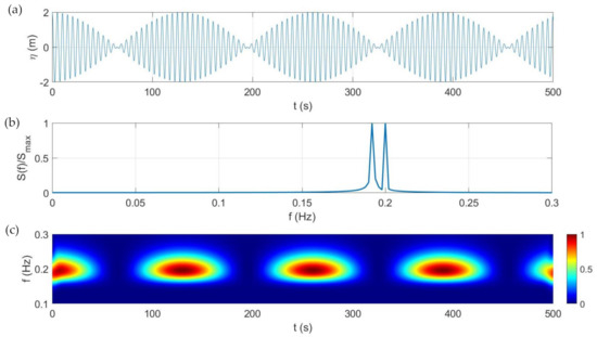
Figure 1.
Wave group signal time series (a) and corresponding spectra using different methodologies: (b) dimensionless Fourier spectrum; (c) dimensionless Wavelet spectrum.
Figure 2 considers the introduction of nonstationarities in the signal of a sine wave. For this purpose, the wave period varied linearly between 5 and 10 s in a time domain of 100 s. Figure 2 shows that the Fourier spectrum does not allow the interpretation of these nonstationary processes, since it does not provide any temporal information concerning the evolution of frequencies and amplitudes. The wavelet analysis provides the variation of frequency over time, accurately evidencing the expected reduction of the frequencies.
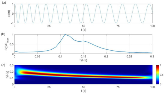
Figure 2.
Nonstationary wave signal time series (a) and corresponding spectra using different methodologies: (b) dimensionless Fourier spectrum; (c) dimensionless wavelet spectrum.
Behind the advantage to analyze signals whose spectral content changes over time, the wavelet analysis does not require defining a cell to interpret the signal. Therefore, when applying this method to retrieve bathymetry from satellite imagery, it is possible to obtain results of the water depth close to the shoreline.
Indeed, as previously described, the use of the FFT method implies the use of cells to estimate the wavelength, whose values are assigned to the center of the cell. If the cells, which have a certain dimension, include an area over shallow water and another located over land, no meaningful results are provided and these cells need to be discarded. Therefore, at the edges of the sea surface in the images there is always a gap (half the size of the cell) associated with the predefined length from the offshore to the nearshore domain at a user-specified spacing. The first and last water depth estimates correspond to the center of the first and last cells and no water depths are determined beyond these positions.
2.3. Sea Surface Synthetic Images
As mentioned before, the linear dispersion relation for ocean gravity waves is applied to retrieve water depths. Our target is to compare and validate the application of the wavelet transform and FFT methods in shallow areas. Often, depth inversions are carried out without the knowledge of the bed profiles. Therefore, we have produced synthetic images of the sea surface that mimic real satellite images (e.g., SAR), using a wave propagation model that describes properly the temporal and spatial variations in the wave height and wave direction over different known bottoms. This highlights the need to use nonlinear models capable of describing nonlinear effects associated with the propagation of water waves in coastal areas.
This work uses the freely available, open-source code FUNWAVE that numerically solves Boussinesq-type equations to model the propagation of water waves. Initially developed by Kirby et al. [26], this fully nonlinear Boussinesq wave model is a phase-resolving numerical approach, time-stepping model for sea surface wave propagation in the nearshore. Together with an adaptive Runge–Kutta time-stepping scheme, the spatial discretization of the used version is done with a MUSCL-TVD finite volume scheme. Details concerning the theory and the numerical implementation of the code can be found in [27].
The wavelengths and directions of swell waves visible in the virtually generated images using the FUNWAVE model were extracted for the subsequent spectral analysis. The propagation of both regular and irregular waves was considered over two different seafloors with 2D and 3D features, respectively, a longshore bar and a headland (Figure 3). The elevation z = 0 corresponds to the mean sea level. This allows assessing the capabilities of the wavelets methodology to provide accurate depth estimations, as well as to evaluate the spatial domain range regarding depth inversion limits.

Figure 3.
Tested seafloors: (a) longshore bar; (b) headland.
The headland was artificially generated but the cross-shore profile with the longshore bar corresponds to a real situation. This change in the seafloor slope and curvature represents a measured cross-shore profile at Costa Nova beach in the Portuguese west coast. This data was obtained online from the COSMO Program (https://cosmo.apambiente.pt/), which was conceived and developed by the Portuguese Environment Agency. This program consists of the collection, processing, and analysis of information on the evolution of beaches, dunes, nearby submarine bottoms, and cliffs along the mainland coast of Portugal. The acquired bathymetric data is obtained with acoustic systems, using both single and multibeam echosounders, which are known to be compliant with international standards, such as the S-44 (Standards for Hydrographic Surveys) developed by the International Hydrographic Organization (IHO). Whenever possible and appropriate, the results are interpreted and compared with those obtained from the use of the FFT methodology, using the algorithm described by [12].
FUNWAVE is widely used for wave research and consultancy practice by scientists and engineers since it is capable of modeling large wavefields. To accommodate variable-resolution grids or boundary-fitting grids, different nesting possibilities can be explored, enabling the capabilities of the code to transfer the results from a coarse grid to a finer grid. In addition, for designing a numerical wave model for operational use, it is important to consider the computing time required for routine applications since it can be greatly affected by the numerical schemes that are used to propagate the waves. This open-source code can be parallelized using MPI (Message Passing Interface), representing an advantage since large-scale simulations can be computationally demanding. Therefore, in our 3D simulations, the code was run on a computing cluster where up to 24 processors were used, significantly reducing the time of the simulations.
3. Results
3.1. Regular Waves
The generation of monochromatic waves using the internal wavemaker of FUNWAVE is very straightforward. Figure 4 shows a first test case where regular waves propagated over a sandbar at normal incidence (i.e., perpendicular to the coastline). With the wavemaker, the simulations considered the propagation of a wave height of H = 2 m and a wave period of T = 10 s.
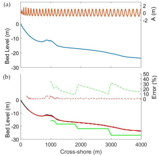
Figure 4.
(a) Regular waves propagating over a sandbar at normal incidence. (b) Real cross-shore profile (black line) versus estimated water depths and respective relative errors using both FFT (green line and green dotted line) and wavelet (red line and red dotted line) methodologies. FUNWAVE numerical simulations performed with H = 2 m, T = 10 s, and a spatial resolution of dx = 1 m. Total simulation time was 2500 s.
In Figure 4a, from right to left, one observes a clear variation of the wave characteristics due to depth-induced changes. Since refraction was absent, the propagation of the waves through shallow waters evidenced shoaling effects. The wave height experienced a small initial decrease, clearly increasing close to the shoreline before breaking. Accordingly, under stationary conditions, to maintain a constant energy flux, this increase in energy density must be compensated with a decrease in wave celerity. Therefore, while the wave period remained constant, shoaling waves exhibited a reduction in wavelength as they propagated into shallower waters.
The calculated water depths using the linear dispersion relation for FFT and wavelet methodologies were applied to the obtained 1D surface elevation pattern. Figure 4b highlights that the relative errors in bathymetric estimation were much smaller in wavelets than in FFT. The use of FFT closer to the coast with a cell of 2000 m led to errors between 3 and 10 m, when compared to the bathymetry used in FUNWAVE. If we increased the cell size, the error became larger (between 10 and 15 m). In both cases, the error increased for greater depths. However, there will always be a limitation to obtain depths close to the shoreline since there will be a gap of half the size of the predefined length of the FFT cells. Therefore, in this case, no water depths were determined in the 1000 m close to the shoreline, using the FFT.
In the case of wavelets, there was practically an overlap between the real cross-shore profile and the estimated depth values, indicating high precision along the entire cross-shore profile with relative errors always below 10%. The errors of less than 0.5 m arise when changes in the seafloor are sudden, such as when a sandbar is present, and very close to the shoreline. Nonetheless, for shallow depths, the sandbar cross-shore position (x = 1000 m) and its morphology were both well reproduced using the wavelet methodology. When compared to the FFT results, there are considerable improvements for the entire spatial domain, which is now significantly expanded.
If the previous harmonic wave approaches the same straight coast previously described, but now at an angle (oblique incidence), the wave slowly changes direction as it approaches the coast due to refraction. This process makes the wave crests bend according to the water depth variations, driving them to become perpendicular to the bathymetric gradient. Simultaneously, as waves travel from deep to shallow water, the shoaling process continues to take place, making the height of swell waves increase and their wavelength decrease.
Figure 5 shows the water depth results for the previous barred beach cross-shore profile, considering parallel depth contours in the longshore direction. The same regular wave (H = 2 m, T = 10 s) was introduced in the internal wavemaker of FUNWAVE, but then the simulation established an angle of propagation of θ = 30°. Therefore, the spatial variation of the wavelength reflects the results of this oblique incidence since both refraction and shoaling processes influence the propagation of these sea surface waves over this variable bathymetry (Figure 5a). The water depth results obtained from the 2D swell wave’s pattern are only shown for the wavelet methodology due to the mentioned inversion limits of the FFT. Figure 5b,c show a very good fit between the FUNWAVE isobaths and the wavelet estimated depths.
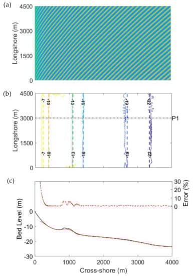
Figure 5.
Regular waves propagating over a sandbar at oblique incidence: (a) generated image representing the two-dimensional wave propagation at the surface; (b) isobaths of the calculated bathymetry (continuous lines) over the FUNWAVE bathymetry (dashed lines); (c) cross-shore profile P1 (real—black line; estimation using wavelets—red line) and respective relative errors. FUNWAVE numerical simulations performed with H = 2 m, T = 10 s, θ = 30°, and dx = 1 m. Total simulation time was 2500 s.
Again, small differences can be observed over the sandbar and near the coastline. Nevertheless, the relative errors over the sandbar were always below 10%, still revealing an interesting fitting using wavelets.
To understand the ability of the wavelet methodology to retrieve bathymetric data from nonuniform stretches of the shoreline, the propagation of oblique waves against a headland was also considered. Figure 6 shows the obtained water depth of a regular wave (H = 2 m, T = 10 s, θ = 30°). The swell wave’s pattern generated with FUNWAVE is presented in Figure 6a. The image evidences the expected wavelength changes due to both shoaling and refraction effects. The simulations clearly indicate that as waves bent towards shallow waters, refraction concentrated and focused the wave energy at the headlands. The retrieved bathymetry shown in Figure 6b reveals a very good adjustment to the real isobaths. We can observe small differences coming from the fluctuation of the estimated values but, in general, the real bathymetry was well reproduced. Even when the bottom slope suddenly changed or presented sharp variations in the coastline orientation, the wavelet analysis successful captured the bathymetric trends (Figure 6c).
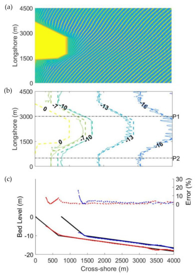
Figure 6.
Regular waves propagating to a headland at oblique incidence: (a) generated image representing the two-dimensional wave propagation at the surface; (b) isobaths of the calculated bathymetry (continuous lines) over the real bathymetry (dashed lines); (c) cross-shore profiles P1 and P2 (real—black lines; estimation using wavelets—red and blue lines) and respective relative errors. FUNWAVE numerical simulations performed with H = 2 m, T = 10 s, θ = 30°, and dx = 1 m. Total simulation time was 2500 s.
3.2. Irregular Waves
Naturally, real ocean waves are always irregular. Irregular waves can be viewed as a sum of many independent regular waves. The wavemaker of FUNWAVE allows considering as input wave bulk parameters or directional spectral data. To simulate a directional sea state, the JONSWAP spectrum was adopted with a peak enhancement factor Υ = 3.3, a wrapped normal directional-spreading function and frequency range of 0.03 Hz to 1 Hz.
When considering the propagation of irregular waves as in the ocean, where the waves present irregular wavelength and height patterns, the direct application of the wavelet transform does not work with the same accuracy as with regular waves. The evaluation of the properties of random waves on a wave-by-wave basis would provide very different wavelength estimates in the analyzed spatial domain. Therefore, it was necessary to explore solutions that would help to solve this problem, testing potential solutions.
Initially, filters were employed, allowing the removal of the short waves. This can be achieved by removing sea patterns from the spectra by filtering out lower wavelengths. Regardless of the cutoff filter, the results revealed a systematic undesirable behavior, that is, good results were only felt in parts of the domain, depending on the adopted values to filter the wavelengths. Smaller cut wavelengths improved results close to shore, but higher values removed data close to shore and only improved offshore. Another solution consisted of applying the wavelet analysis to spatial subdomains instead of performing the analysis on the entire spatial domain. Various tests of sensitivity were performed to establish the size and spacing of the subdomains. Although better results were obtained, this solution still did not provide results close to the expected acuity.
It was concluded that by simultaneously performing an analysis through subdomains and using filters, the results of the methodology were optimized. Nevertheless, in some points of the spatial domain, it was found that some estimated wavelength values revealed sudden unrealistic changes, differing significantly from other estimations. The solution found to remove these outliers was to use the median in the analysis process. The median is a robust statistical estimator capable of coping with outliers, allowing automatically extracting these anomalous wavelength estimations in each analyzed cell.
With these changes introduced in the wavelet methodology, simulations were carried out for the two previous different bathymetries where irregular waves were generated according to a JONSWAP spectrum with a significant wave height of Hs = 2 m and a peak period of Tp = 10 s. The results, shown in Figure 7 and Figure 8, reveal some errors in the estimation of the nearshore bathymetry, but still are quite satisfactory.
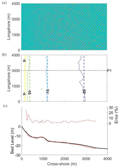
Figure 7.
Irregular waves propagating over a sandbar at oblique incidence: (a) generated image representing the two-dimensional wave propagation at the surface; (b) isobaths of the calculated bathymetry over the real bathymetry; (c) cross-shore profile P1 (real—black line; estimation using wavelets—red line) and respective relative errors. FUNWAVE numerical simulations performed with Hs = 2 m, Tp = 10 s, θ = 30°, and dx = 1 m. Total simulation time was 2500 s.
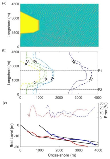
Figure 8.
Irregular waves propagating to a headland at oblique incidence: (a) generated image representing the two-dimensional wave propagation at the surface; (b) isobaths of the calculated bathymetry over the real bathymetry; (c) cross-shore profiles P1 and P2 (real—black lines; estimation using wavelets—red and blue lines) and respective relative errors. FUNWAVE numerical simulations performed with Hs = 2 m, Tp = 10 s, θ = 30°, and dx = 1 m. Total simulation time was 2500 s.
In Figure 7, the calculated isobaths are roughly disposed parallel to the coast and the sandbar is also reproduced. The errors increase for higher water depths, with relative errors always below 10%, representing errors below 2 m.
In Figure 8, the calculated isobaths also present the expected contour of the headland and the slope changes are replicated. In general, the elevation errors are small, increasing for higher depths and close to the shore reaching relative errors of 20%.
4. Discussion
The numerical simulations demonstrate the wavelet methodology overcomes the FFT limitations, where the simulated bathymetry slightly deviates from the real bathymetry even creating a realistic sea state as input to these simulations. It is noteworthy to mention the simulations include comparisons for water wave propagation over variable bathymetries and the wavelet analysis allows retrieving bathymetric data along the entire cross-shore profiles. For the benchmark test considered, the bathymetric estimates with wavelet methodology present very small errors when compared with the FFT.
Close to the shoreline, the FFT cannot provide depth estimates since there will be a gap of half the size of the predefined length of the FFT cells. The wavelet methodology allows retrieving bathymetric data along the entire cross-shore profiles, clearly expanding the results for shallower depths. Still, very close to the shoreline, the bathymetric estimates present larger errors, with relative errors generally below 20%, which can be associated with wavelet boundary value problems (e.g., [28]) or to the validity of the linear dispersion relation (e.g., [29,30]). Indeed, in shallow water waves, the wave profile becomes nonlinear and finite amplitude effects became important. For such waves, celerity and wavelength are affected by wave height and the validity of the linear dispersion relation is questionable. Using nonlinear amplitude-dependent dispersion relations, especially as water depth decreases, deserves further investigation in the future.
The errors also increase for higher water depths. As mentioned by [12], an increase of relative errors is expected for higher depths. This conclusion was achieved by studying the uncertainty to evaluate the relative error depending on the accuracy of the computed wavelength used in the linear dispersion relation.
It is also observed when the seafloor suddenly changes, such as when a sandbar is present, the errors also increase in that region. This can be caused by the influence of wavelength changes caused by sudden bottom shape changes in shallow depths where the accuracy of the linear dispersion relation could be also improved using high-order dispersion relation models [29]. Despite these limitations, the wavelet methodology in conjunction with the linear dispersion relation still provided interesting fits to the real bathymetry.
It is noted that the passage from regular to irregular waves introduces major challenges to retrieve bathymetric data. The superposition of a number of harmonic waves with different frequencies and amplitudes raises difficulties to retrieve wavelength values. This is important to mention since satellite images capture real ocean waves, which are always irregular. Therefore, it is expected that a real image of the sea surface would not present as clear a regular wave pattern as for regular waves. It was concluded that by performing an analysis through subdomains with the use of filters and the removal of outliers, the results of the methodology can be optimized.
The difficulties of irregular waves became apparent in the headland considered in Figure 8, where the worse outcomes regarding the retrieved estimated depths can be associated with the used filters or with the existence of wave groups that, as explained through Figure 1, will present a variation in the magnitude intensity that alternately increases and decreases. Therefore, the constructive and destructive interference of the waves will, respectively, evidence or attenuate the appearance and detection of the respective wavelength peaks in the image spectra.
5. Conclusions
The determination of the seafloor bathymetry from remote sensing imagery presents a rather easier process to explore potentially widespread areas. The changes in the sea surface evidenced by the swell wave’s pattern in the nearshore, based on its roughness and height, are directly linked with the local bathymetry.
This work considers a wavelet spectral analysis to obtain bathymetric data. This new imaging methodology is explored over different known bottoms, with 2D and 3D features such as longshore bars or headlands. The characteristics of the wave propagation are simulated in a numerical Boussinesq-type model, forced with both regular and irregular waves. The generated images of the water surface are extracted from the model results for the subsequent wavelet spectral analysis. The estimated depths are compared with the bathymetry inserted in the numerical model.
For regular waves, excellent results are obtained for the wavelet methodology. When compared to the FFT results, there are considerable improvements for the entire spatial domain, significantly reducing the errors of the retrieved depths. In addition, the wavelet analysis allows expanding the analysis for shallower depths. The direct application of the wavelet transform for irregular waves does not work with the same accuracy as for regular waves. The results of the applied spectral analysis can be optimized by simultaneously performing an analysis to subdomains and adopting filters. By doing so, the wavelet image processing methodology shows very promising results over variable bathymetries.
The observed capabilities of this new methodology justify additional work to map shallow marine environments from satellite images that enable retrieving the wave field (e.g., Sentinel-1).
This work explored the spatial variation of the wavelength associated with both refraction and shoaling processes. Nevertheless, the tested waves were always breaking close to the shoreline. This process was not explored with this new methodology but, in the future, it can be studied in conjunction with nonlinear amplitude-dependent dispersion relation to improve the results at shallower depths. Also, in the analysis, we have considered swell waves, but satellite images can also evidence surface patterns associated with different sea states (e.g., locally generated wind waves). The application of this methodology to such images presents an additional challenge that deserves to be further studied.
Author Contributions
Conceptualization, D.S., T.A., and P.A.S.; methodology, D.S., T.A., and P.A.S.; software, D.S.; validation, D.S., T.A., and P.A.S.; formal analysis, D.S., T.A., and P.A.S.; investigation, D.S., T.A., P.A.S., and P.B.; resources, D.S.; data curation, D.S., T.A., P.A.S., and P.B.; writing—original draft preparation, D.S. and T.A.; writing—review and editing, D.S., T.A., P.A.S., and P.B.; visualization, D.S. and T.A.; supervision, T.A. and P.A.S.; project administration, P.B.; funding acquisition, P.B. All authors have read and agreed to the published version of the manuscript.
Funding
This research was funded by Direção Geral da Política do Mar, through project NAVSAFETY of the Fundo Azul program. Thanks are due to FCT/MCTES for the financial support to CESAM (UIDP/50017/2020+UIDB/50017/2020), through national funds.
Acknowledgments
The authors gratefully acknowledge Luís Carvalheiro for his help and access to the High Performance Computational System (ARGUS) at University of Aveiro, enabling running the numerical model on a computing cluster, significantly reducing the time of the simulations.
Conflicts of Interest
The authors declare no conflict of interest.
References
- Jawak, S.D.; Vadlamani, S.S.; Luis, A.J. A Synoptic Review on Deriving Bathymetry Information Using Remote Sensing Technologies: Models, Methods and Comparisons. Adv. Remote Sens. 2015, 4, 147–162. [Google Scholar] [CrossRef]
- Bergsma, E.W.J.; Almar, R.; Maisongrande, P. Radon-Augmented Sentinel-2 Satellite Imagery to Derive Wave-Patterns and Regional Bathymetry. Remote Sens. 2019, 11, 1918. [Google Scholar] [CrossRef]
- Botha, E.; Brando, V.; Dekker, A.; Botha, E.J.; Brando, V.E.; Dekker, A.G. Effects of Per-Pixel Variability on Uncertainties in Bathymetric Retrievals from High-Resolution Satellite Images. Remote Sens. 2016, 8, 459. [Google Scholar] [CrossRef]
- Evagorou, E.G.; Mettas, C.; Agapiou, A.; Themistocleous, K.; Hadjimitsis, D.G. Bathymetric Maps from Multi-Temporal Analysis of Sentinel-2 Data: The Case Study of Limassol, Cyprus. Adv. Geosci. 2019, 45, 397–407. [Google Scholar] [CrossRef]
- Sagawa, T.; Yamashita, Y.; Okumura, T.; Yamanokuchi, T.; Sagawa, T.; Yamashita, Y.; Okumura, T.; Yamanokuchi, T. Satellite Derived Bathymetry Using Machine Learning and Multi-Temporal Satellite Images. Remote Sens. 2019, 11, 1155. [Google Scholar] [CrossRef]
- Almar, R.; Bergsma, E.W.J.; Maisongrande, P.; de Almeida, L.P.M. Wave-Derived Coastal Bathymetry from Satellite Video Imagery: A Showcase with Pleiades Persistent Mode. Remote Sens. Environ. 2019, 231, 111263. [Google Scholar] [CrossRef]
- Young, I.R. Wind Generated Ocean Waves, 1st ed.; Elsevier Ocean Engineering Book Series: Amsterdam, The Netherlands, 1999; Volume 2, pp. 1–288. [Google Scholar]
- Bergsma, E.W.J.; Almar, R. Video-based depth inversion techniques, a method comparison with synthetic cases. Coast. Eng. 2018, 138, 199–209. [Google Scholar] [CrossRef]
- Salameh, E.; Frappart, F.; Almar, R.; Baptista, P.; Heygster, G.; Lubac, B.; Raucoules, D.; Almeida, L.P.; Bergsma, E.W.J.; Capo, S.; et al. Monitoring Beach Topography and Nearshore Bathymetry Using Spaceborne Remote Sensing: A Review. Remote Sens. 2019, 11, 2212. [Google Scholar] [CrossRef]
- Brusch, S.; Held, P.; Lehner, S.; Rosenthal, W.; Pleskachevsky, A. Underwater bottom topography in coastal areas from Terra SAR-X data. Int. J. Remote Sens. 2011, 32, 4527–4543. [Google Scholar] [CrossRef]
- Mishra, M.K.; Ganguly, D.; Chauhan, P.; Ajai. Estimation of coastal bathymetry using RISAT 1 C-band microwave SAR data. IEEE Geosci. Remote Sens. Lett. 2014, 11, 671–675. [Google Scholar] [CrossRef]
- Pereira, P.; Baptista, P.; Cunha, T.; Silva, P.A.; Romão, S.; Lafon, V. Estimation of the Nearshore Bathymetry from High Temporal Resolution Sentinel-1A C-Band SAR Data—A Case Study. Remote Sens. Environ. 2019, 223, 166–178. [Google Scholar] [CrossRef]
- Tuteur, F.B. Wavelet Transformations in Signal Detection. IFAC Proc. 1988, 21, 1061–1065. [Google Scholar] [CrossRef]
- El-Diasty, M.; Al-Harbi, S. Development of wavelet network model for accurate water levels prediction with meteorological effects. Appl. Ocean Res. 2015, 53, 228–235. [Google Scholar] [CrossRef]
- El-Diasty, M. Satellite-Based Bathymetric Modeling Using a Wavelet Network Model. ISPRS Int. J. Geo. Inf. 2019, 8, 405. [Google Scholar] [CrossRef]
- Sancho, F.; Abreu, T.; D’Alessandro, F.; Tomasicchio, G.R.; Silva, P.A. Surf hydrodynamics in front of collapsing coastal dunes. J. Coast. Res. 2011, 1, 144–148. [Google Scholar]
- Abreu, T.; Silva, P.A.; Baptista, P.; Pais-Barbosa, J.; Fernández-Fernández, S.; Ferreira, C.; Matos, J. Analysis of Nonlinear Wave Parameters on Ofir Sandy Beach (NW Portugal). In Advances in Natural Hazards and Hydrological Risks: Meeting the Challenge; Fernandes, F., Malheiro, A., Chaminé, H., Eds.; Springer: Cham, Switzerland, 2020; pp. 147–151. [Google Scholar]
- Pacheco, A.; Horta, J.; Loureiro, C.; Ferreira, Ó. Retrieval of nearshore bathymetry from Landsat 8 images: A tool for coastal monitoring in shallow waters. Remote Sens. Environ. 2015, 159, 102–116. [Google Scholar] [CrossRef]
- Pushparaj, J.; Hegde, A.V. Estimation of bathymetry along the coast of Mangaluru using Landsat-8 imagery. Int. J. Ocean Clim. Syst. 2017, 8, 71–83. [Google Scholar] [CrossRef]
- Abreu, T.; Matos, J.; Pereira, P.; Cunha, T.R.; Baptista, P.; Silva, P.A. Acquisition of Bathymetric Data from Satellite Images. In Proceedings of the 8th SCACR—International Short Course/Conference on Applied Coastal Research, Santander, Spain, 3–6 October 2017. [Google Scholar]
- Pleskachevsky, A.; Lehner, S.; Heege, T.; Mott, C. Synergy and Fusion of Optical and Synthetic Aperture Radar Satellite Data for Underwater Topography Estimation in Coastal Areas. Ocean Dyn. 2011, 61, 2099–2120. [Google Scholar] [CrossRef]
- Lehner, S.; Pleskachevsky, A.; Bruck, M. High-resolution satellite measurements of coastal wind field and sea state. Int. J. Remote Sens. 2012, 33, 7337–7360. [Google Scholar] [CrossRef]
- Wiehle, S.; Pleskachevsky, A. Bathymetry Derived from Sentinel-1 Synthetic Aperture Radar Data. In Proceedings of the 12th European Conference on Synthetic Aperture Radar Electronic, Aachen, Germany, 4–7 July 2018. [Google Scholar]
- Zieliński, T. Wavelet transform applications in instrumentation and measurement: Tutorial and literature survey. Metrol. Meas. Syst. 2004, 11, 61–101. [Google Scholar]
- Shyu, H.; Sun, Y. Construction of a Morlet Wavelet Power Spectrum. Multidimens. Syst. Signal Process. 2002, 13, 101–111. [Google Scholar] [CrossRef]
- Kirby, J.T.; Wei, G.; Chen, Q.; Kennedy, A.B.; Dalrymple, R.A. FUNWAVE 1.0, Fully Nonlinear Boussinesq Wave Model, Documentation and User’s Manual, ReportCACR98-06; Center for Applied Coastal Research, Department of Civil and Environmental Engineering, University of Delaware: Newark, NJ, USA, September 1998. [Google Scholar]
- Shi, F.; Kirby, J.T.; Harris, J.C.; Geiman, J.D.; Grilli, S.T. A high-order adaptive time-stepping TVD solver for Boussinesq modeling of breaking waves and coastal inundation. Ocean Model. 2012, 43–44, 36–51. [Google Scholar] [CrossRef]
- Bertoluzza, S.; Naldi, G.; Ravel, J.C. Wavelet Methods for the Numerical Solution of Boundary Value Problems on the Interval. Wavelet Anal. Appl. 1994, 5, 425–448. [Google Scholar] [CrossRef]
- Ge, H.; Liu, H.; Zhang, L. Accurate Depth Inversion Method for Coastal Bathymetry: Introduction of Water Wave High-Order Dispersion Relation. J. Mar. Sci. Eng. 2020, 8, 153. [Google Scholar] [CrossRef]
- Flampouris, S.; Seeman, J.; Ziemer, F. Sharing our Experience Using Wave Theories Inversion for the Determination of the Local Depth. In Proceedings of the OCEANS 2009-EUROPE Conference, Bremen, Germany, 11–14 May 2009. [Google Scholar] [CrossRef]


© 2020 by the authors. Licensee MDPI, Basel, Switzerland. This article is an open access article distributed under the terms and conditions of the Creative Commons Attribution (CC BY) license (http://creativecommons.org/licenses/by/4.0/).