Abstract
The ability to accurately predict beach morphodynamics is of primary interest for coastal scientists and managers. With this goal in mind, a stochastic model of a sandy macrotidal barred beach is developed that is based on cross-shore elevation profiles. Intertidal elevation was monitored from monthly to annually for 19 years through Real Time Kinematics-GPS (RTK-GPS) and LiDAR surveys, and monthly during two years with an RTK-GPS. In addition, during two campaigns of about two weeks, intensive surveys on a daily basis were performed with an RTK-GPS on a different set of profiles. Based on the measurements, space and time variograms are constructed in order to assess the spatial and temporal dependencies of these elevations. A separable space-time covariance model is then built from them in order to generate a large number of plausible future profiles at arbitrary time instants , starting from observed profiles at time instants t. For each simulation, the total displaced sand volume is computed and a distribution is obtained. The mean of this distribution is in good agreement with the total displaced sand volume measured on the profiles, provided that they are lower than 45 m/m. The time variogram also shows that 90% of maximum variability is reached for a time interval of three years. These results demonstrate how the temporal evolution of an integrated property, like the total displaced sand volume, can be estimated over time. This suggests that a similar stochastic approach could be useful for estimating other properties as long as one is able to capture the stochastic space-time variability of the underlying processes.
1. Introduction
Beaches act as a natural buffer to protect hinterland against significant waves and coastal erosion as well as flooding. Understanding and predicting coastal morphodynamics are critical for the safety of the existing ecosystems, infrastructures, and for mitigating expected damages from future changes. Morphodynamics of beach can also affect the biodiversity and biological component, like, e.g., nesting ecology of sea turtles, burrowing of bivalves and presence of sand crabs [1,2,3]. However, prediction of beach morphology remains a challenge due to the complex processes between forcing factors and sediment transport occurring on a broad range of temporal and spatial scales. These processes can involve regular seasonal events (tidal cycles, current patterns) or stochastic events, like storms. Inherent interactions between evolving morphological features, such as intertidal sand bars and external forcings, produce both linear and nonlinear feedback mechanisms [4]. The beach profile response may be related to the existing coastal state and to the forcings operating on varied spatial and temporal scales [5,6,7]. On short-time scale, ranging from hours to months, wave storms hitting the coast may be the dominant processes that impact the beach changes and sediment transport processes, while sea level change and sediment fluxes play a more important role on longer-time scale. In developing models for predicting beach morphology, it is thus crucial to distinguish between behaviour and evolution.
Over the last decades, complex process-based morphological models have been developed to simulate and predict beach morphological changes (e.g., [8,9,10]). Although they have performed well for short-term predictions, their computational costs, modelled instability, and misspecifications of the physics conditions prevent them from reproducing beach evolution. Therefore, morphological tendencies that are observed in practice are often difficult to model reliably [11]. This has encouraged the development of data-driven models that are statistical methods whose entire structure and associated parameters are estimated directly from the objective analysis of observational data. General characteristics of the natural system, such as beach width, volume, and slope, are deduced only based on data analysis without considering other sources of information about the system [12]. The key advantage is that no prior knowledge of the system dynamics is required which is appropriate when the dynamics are not fully understood, as well as their long-term simulation stability and robustness [13]. Stochastic approaches for assessing beach changes have been modeled early while using Markov-type processes [14,15]. Geostatistical estimation of beach properties that are based on variogram method [16], linear [4], and nonlinear [17,18,19] data-based modelling techniques have been applied in the past in order to investigate beach morphology, mostly in a purely spatial mapping framework. Additionally, the beach equilibrium model is another parametric method which has been widely accepted and often used as a proxy for shoreline (e.g., [20,21,22]) and more recently to study the variation of beach profile position [23]. The success of data-based modelling depends on the total size of the observational data set, characterized by its specific spatial coverage, its spatial and temporal resolution and its overall length in time. A blind testing comparison of various models (ranging from established models to machine learning algorithms) making use of cross-shore profiles or shorelines is provided by Montaño et al. [24].
As emphasized by [25], two approaches have been generally adopted to better study beach morphodynamics: long-term approach that is based on seasonal to decadal data, and recovery from dramatic events. This study focuses on the morphodynamics of sandy beaches characterized by an intertidal bars-trough system commonly found along meso- and macro-tidal environments by taking advantage of high-quality data sets (with high spatial resolution and a combination of low to high temporal resolutions) over a time span of 19 years along the Belgian coast. The aim is to investigate the benefit of using a space-time stochastic modeling approach to capture both the spatial variability and temporal evolution of the beach elevation along profiles. Proxies of the beach evolution, such as dune foot position, limit of wet and dry sand, shoreline position, or isocontours (e.g., [26,27,28]) are out of reach, as our dataset is restricted to one dimensional measurements repeated along the same few cross-shore profiles over time. The developed space-time model is thus used to predict the integrated sand volume change over time along these profiles. Relationships between the morphological development of the multi-barred beaches and controlling factors as meteo-marine conditions will be subject of future studies, as the main goal of the paper is to assess the ability of such a space-time model to predict sand volume change from data that where mostly sampled every few months, thus precluding the direct use of the direct use of meteo-marine factors at a much finer time scale, as done in [25]. As noted by [16], accurate sand volume estimation is required to monitor rates of beach erosion and accration, so sand volume change assessment is particularly relevant for beach preservation and management.
2. Study Site
The North Sea is an arm of the Atlantic Ocean, with a majority of ocean current coming from the northwest opening, while a lesser portion of warm current comes from the English Channel. The main flow pattern of water is an anti-clockwise rotation along its edges. The fetch length is limited so that wave period is shorter, and amplitudes are higher than in deep ocean water, as the North Sea is located on the continental shelf. The Belgian coast is boarding the east part of North Sea and is about 65 km long, mainly oriented from South-West (SW) to North-East (NE). The typical wind speed is about 8 m/s, with winds most frequently coming from SW. The time averaged significant wave height is about 100 cm, with typical wave period of about 6 s. Most of the time waves and winds come from the same direction. Waves that propogate in the shallow Belgian coastal zone are transformed due to the interaction with the sea bottom, so that wave climate varies from place to place. Frequent storms occur during the winter months, where most severe events are characterized by wave heights exceeding 4 m and storm duration of more than 30 h. For several centuries, anthropogenic activities along the Belgian coastline have attempted to reshape the coast to maintain the coastline position, or even to claim land from the sea, so that the natural interaction between the beach and coastal dunes has been disrupted. The protection of the Belgian coastline is a combination of natural and artificial defence [29]. Nowadays, 60% of the coast has a hard coastal protection with seawalls, revetments and groynes [30]. Belgian beaches mainly consist of fine to medium sand and mainly characterized by quartz enriched by calcareous particles, with an average median grain size of 200–220 m and a cross-shore variation in median grain size of 160–380 m. Sediments tend to become coarser from the west to the east [31].
Our study site is located at Groenendijk beach (sections 48–50, as defined by the Coastal Division of the Flemish Authority) situated in the western part of the Belgian coast (Figure 1). This part of the coast is oriented SW-NE and is characterized by sandy dissipative beaches (surf scaling parameter >20) with a gentle slope of less than 1% and a width >300 m. There is a northeastward longshore sediment drift in this zone, with a total longshore SW-NE transport evaluated at 145,000 m/year along the Belgian coast [32]. The beach is backed by well-developed coastal dunes of 10 m TAW (Tweede Algemeene Waterpassing, the Belgian datum tied to the lowest spring tide in Ostend). Several large shallow sand banks (known as the Flemish banks) can be found offshore on the shallow continental shelf (−3 m TAW). They dissipate part of the wave energy and, thus, contribute to lower wave height reaching the beaches [33]. The coast experiences a macro-tidal regime with a tidal range from 3 to 5 m [34]. During energetic events, storm surge is over 1.0 m. The onshore wave buoy at Trapegeer, located 7 km offshore and at −10 m TAW, has a mean significant wave height around 0.6 m with a period of 3–4 s. Wave direction measured at Kwintebank wave buoy, which is 15 km offshore and at −3.5 m TAW, is characterized by two dominant wave directions coming primarily southwest and to a lesser extent northeast.
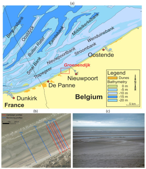
Figure 1.
Location of study site and cross-shore profiles. (a) Study site position on the Belgian Coast. (b) Continuous monitoring profiles (in blue), campaign profiles (in red), intertidal zone (between dashed lines). (c) Photo of the Groenendijk beach showing the intertidal bars.
This beach is characterized by a multiple intertidal bar-trough system, also called a ridge and runnel beach, as classified by [35]. In general, the system consists of three to five parallel bars between the high and low water lines (Figure 2). In general too, bars and troughs are continuous in alongshore direction, except when intertidal drainage channels are present. These features are separated by an average distance of 90 m cross-shore and an average bar-trough amplitude of 60 cm. Though no data are available for the submerged area in this study, it is worth noting that the bar system generally extend beyond the intertidal zone, with subtidal bars that play an important role in dissipating wave energy. The intertidal beach is composed of fine to medium sand with a median diameter of 200 m. The beach has prograded at a rate of about 21 m/m·y (cubic meters per meter width and per year) over the last decades [36].
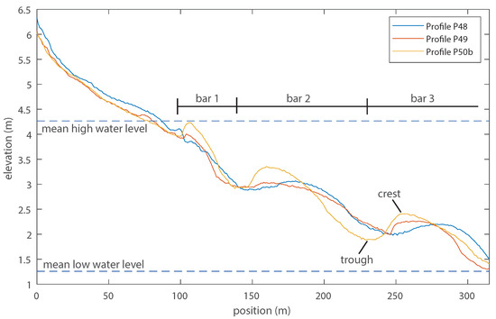
Figure 2.
An example of three cross-shore Coastal Division profiles (out of the five) sampled at the same date, emphasizing the presence of sand bars over all profiles as well as the variability between profiles.
3. Material and Methods
3.1. Monitoring Profiles
Elevation measurements that were obtained along profiles P48 to P50c were surveyed by the Coastal Division of the Flemish Authority in order to monitor changes in beach volume over time. Surveys were carried out on a monthly basis between February 2017 and May 2019 while using a Real Time Kinematics (RTK) GPS system, except in November 2017 and in summers. No survey was completed in summer season (i.e., in July–August due to the touristic season) and in November 2017. The distance between profiles range from 50 m to 240 m (see Figure 1). The location of these profiles depends on the monitoring sections, as delimited by the Coastal Division. All of the profiles start at a fixed location near the dune toe and are covering the first three bars of the intertidal zone. No measurements were made for the submerged zone. The Root Mean Square Error (RMSE) was about 2.5 cm in vertical and horizontal directions. In general, distances between successive measurements varied from 5 to 20 m, with an average distance of about 15 m. Profiles were rebuilt at 1 m spacing resolution with unmodified Akima spline interpolation function [37]. This function was compared to other splines and selected as it had the best fit and no overshooting effect. An example of these profiles is given in Figure 2.
In addition, airborne Light Detection And Ranging (LiDAR) surveys were commissioned by Coastal Division on a yearly basis between 2000 and 2012, and carried out twice per year between 2013 and 2019. LiDAR surveys were conducted during low spring tides in order to cover a large part of the beach. A timeline of these surveys is presented in Figure 3 and the exact dates are given in Table 1. Each survey provided a three-dimensional (3D) (horizontal position and vertical elevation) cloud of points over the emerged and intertidal zone of the beach, with a density ranging from one to five points per square meter. RMSE of LiDAR is reported to be equal to 2 cm under test conditions. The point clouds were used to produce Triangulated Irregular Networks (TIN) that were converted afterwards to raster Digital Terrain Models (DTMs) at a resolution of 25 cm. The elevations were extracted from the DTMs along the P48 to P50c profiles at the same 1 m spacing than for the RTK GPS data. Thus, combining these LiDAR and RTK GPS data provides a set of five profiles where elevation is measured at a 1 m spacing at 54 distinct dates from 2000 to 2019, with data from years 2000 to 2016 that are only coming from LiDAR measurements, while data for years 2017 to 2019 are coming both from LiDAR and RTK GPS measurements.
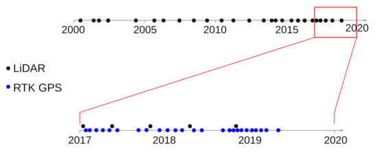
Figure 3.
Timeline of the monitoring surveys used in this study. Top: LiDAR surveys since 2000. Bottom: detail of the timeline with RTK GPS (blue) and LiDAR (black) surveys since 2017.

Table 1.
Timeline of the monitoring surveys used in this study. Italicized dates correspond to the surveys for the CREST campaigns.
3.2. Campaign Profiles
Extra elevation profiles were obtained in the framework of the Climate Resilient Coast project between 2015 and 2019 (http://www.crestproject.be). Two campaigns were performed at the study site. The profiles were surveyed every day for eight and ten days, respectively, in January and November 2018. Cross-shore elevation of the beach was measured along five profiles in section 50 of the beach (Figure 1b) using an RTK GPS in walking mode to automatically measure elevation with 1 m measurement interval. Benchmarks that were near the dune toe were used to ensure that sampled positions along the profiles were the same for all dates. Profiles were not interpolated due to the high density of measurements. Similarly, measurements are only covering the emerged and intertidal zones.
3.3. Average Profiles and Progradation
In order to study the space-time dynamics of the profiles over time, we will first investigate the long-term evolution of profiles over time. Consider that is the measured elevation at position x along a given profile at a time instant t. Thus, we can characterize the long term evolution at any location x by the mean function , where refers to the expectation. We will consider here that , where is a time-invariant mean profile while the second term quantifies the linear progradation over time, with parameters and that depend on the position x along the profile. From the data at hand, it is easy to estimate and by looking at the values along the time axis for every position x. Substracting this progradation effect allows for us to obtain . These time-invariant mean profiles can then easily be compared and progradation rates can be integrated to obtain the beach progradation rate , with
where is usually expressed in m/m·y. It is worth noting that we only consider here a linear progradation over time, but more elaborate temporal evolution could be used if relevant, of course.
3.4. Spatial/Temporal Variograms
Assessing the way that elevation changes over time and along these profiles is done by relying on the spatial and temporal variograms. To the opposite of previous studies related to the use of these tools in beach studies (see e.g., Swales [16], Dolan et al. [38], Harley et al. [39]) that were restricted to separate spatial and temporal analyses in a mapping framework, we will consider both space and time together. Consider that is the measured elevation at position x along a given profile at a time instant t. It is characterized by a mean elevation (after correcting for progradation) that depends on the position x along the profile. The variation of elevation around this mean profile is denoted . The spatial and temporal variograms are then, respectively, defined as
where h is the distance separating two locations and is the time lag separating two measurements. These variograms measure the dissimilitude between measurements, either as a function of the distance h or the time lag that separates them. For measurements that can be considered to be zero-mean and second-order stationary over space and time, they are linked to the traditional covariance functions and , which are defined as
so that and , where is the variance of the measurements. These covariance functions are also related to the correlation functions and , with and . More details can be found in [40,41] about the properties and the estimation of these various functions. The main advantage of the variogram is to allow for the user to interpret the extent of the spatial/temporal dependence based on the shape of the function, as illustrated in Figure 4. The distance/time lag that is needed to reach 95% of the variance is called the range r of the variogram. It corresponds to the distance/time lag beyond which no significant correlation exists. Measurements separated by at least this range can be considered statistically unrelated for practical purposes. The vertical jump at the origin of the function is called the nugget effect and corresponds here to the variance of the measurement errors (i.e., the errors that are associated with the RTK GPS and LiDAR systems). If a periodic spatial/temporal behaviour is present in the measurements, it will be translated as a periodic behaviour as well in the corresponding spatial/temporal variograms and covariance functions. There is a direct connection with spectral theory, as the power spectral density is the Fourier transform of the covariance function (see e.g., Jenkins and Watts [42]), which is itself linearly related to the variogram. When it comes to relating beach profiles to various scales, alternate approaches, like wavelet analysis, could be relevant (see e.g., Li et al. [43]).
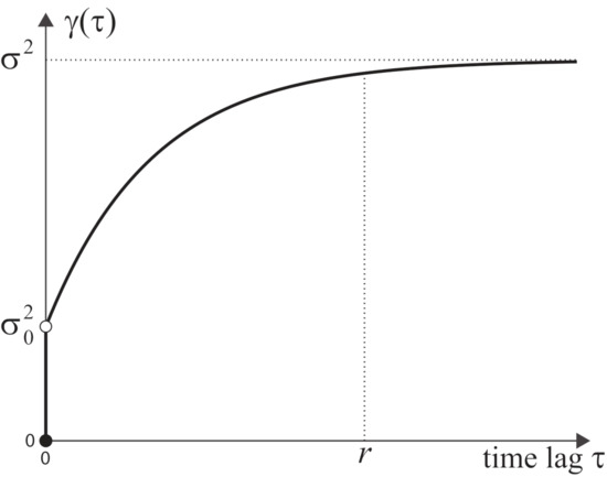
Figure 4.
Generic features for a temporal variogram , showing the variance , the nugget effect and the range r. The same generic features are relevant for a spatial variogram in general.
3.5. Space-Time Model and Simulations
Elevation change needs to be statistically assessed in space and time together. This requires a space-time (ST) covariance model combining the spatial and temporal correlation functions. Such a ST model is given by the separable covariance model
that combines in a simple way the correlation functions and that were defined separately over space and over time, respectively. This model provides the covariance matrix for any vector of positions and time instants. Instead of using this space-time model for doing spatial interpolation or temporal prediction (i.e., using classical kriging algorithms as usually done), we will use it instead in a conditional simulation framework for assessing the volume changes over time along a cross-shore profile.
Given two time instants t and , the vector is defined as the elevations that are measured along a given profile at the time instant t, with . Similarly, the vector contains the elevations measured at the same set of n locations but at the time instant . Clearly, the spatial covariance matrix for both and is the same and it only depends on the spatial covariance function . Moreover, from Equation (1), the covariance matrix between and is given by . Consequently, the covariance matrix for the stacked vector that involves the elevation at two time instants that are separated by a time lag is then given by
This ST covariance matrix is at the root of any simulation procedure that simultaneously involves the elevation measurements at the same positions along the profile at two time instants t and . Starting from observed elevations at time t, it is thus possible to simulate elevations at time by accounting for the ST dependence between all measurements as given by . Repeating this several times produces a distribution of simulated profiles at . If and are assumed to be jointly Gaussian random vectors, simulations are easy to implement. Indeed, what is sought for is the conditional distribution of possible random vectors at time , given that has been observed at time t.
In statistical theory, if one assumes, in general, a Gaussian random vector where and , it then comes that
Using now a Choleski decomposition of the matrix, such that where is a lower triangular matrix, it is easy to simulate a random vector having the properties specified in Equation (3), with
where is a vector of independent zero-mean unit variance Gaussian distributed values, which can obtained from any random number generator, and where . Using Equation (4) repeatedly allows for simulating an arbitrary large number of independent profiles, which are all conditioned on the same initial observed profile and obey the properties given in Equation (3). In other words, all of the simulated ’s are plausible elevation profiles at time instant . They are all consistent both with the observed values at time t and with the covariance model specified in Equation (1).
4. Results
Most of the results thatare presented here are based on analyses conducted jointly on the five monitoring profiles P48 to P50c, covering a time span of 19 years. The 1 m spacing elevations as interpolated from the Akima splines are used in all subsequent analyses. The campaign profiles, which are covering a time span of only few days, are only used for aspects related to the estimation of the temporal variogram.
Depending on the date and the time of measurements, the length of the profiles built by combining LiDAR and RTK GPS measurements may vary. In order to process comparable measurements for all profiles, only the first 316 meters have been considered for the subsequent computations. They all covered the emerged and major part of the intertidal zone of the beach, which can extend close to 400 m at some dates.
4.1. Average Profiles and Progradation
The mean elevations of the five profiles surveyed at the same 54 dates were first computed in order to investigate the dynamic of the bars over time and along the profiles. The sampling frequencies ranged from a few days to two years (with a yearly average sampling frequency from 2000 to 2016 and a monthly average sampling frequency from 2017 to 2019). Accordingly, for a given position along the profile, the elevation at each date was weighted by the average time that separates it from the previous and next sampling dates (i.e., the closer two dates are, the lower is their weight). The corresponding weighted mean of the elevation over time was computed every meter along each of the 5 profiles, thus yielding five temporally averaged profiles that are presented in Figure 5.
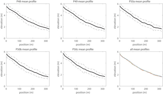
Figure 5.
Average Coastal Division profiles as computed from a weighted mean of the elevation measured at 54 dates (plain line), along with the standard deviation of the measurements (dashed line). The last figure shows all average profiles as superimposed for comparison purpose.
Although bar systems appear clearly on any single profile at any date, these features do not appear anymore on the average profiles. The average profiles also do not differ from each other. The magnitude of the variations around the average profile (as measured by the variance of the elevations around the mean profile) is similar for all positions along the profile, with an estimated value = 0.0510 m. This emphasizes the fact that, even if the bars and troughs are ubiquitous features, their position is subject to major changes over a time span of several years (see Section 4.2). Interpolating all of the profiles at the same location for all dates makes possible to look at the time series of elevations at any chosen position, as presented in Figure 6. The results indicate that a progradation mainly occurs close to the dunes, where elevation increases over time. The amount of beach progradation can be assessed from the slope of the regression line fitted on these time series, at each position and for the five profiles (Figure 7).
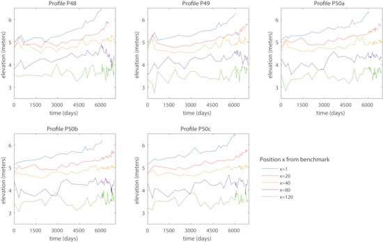
Figure 6.
Time series of elevation at a set of chosen positions x along the Coastal Division cross-shore profiles (where corresponds to the benchmark at the dune toe), showing that progradation (as quantified by the slope of the time series) mainly occurs close on the upper beach part.
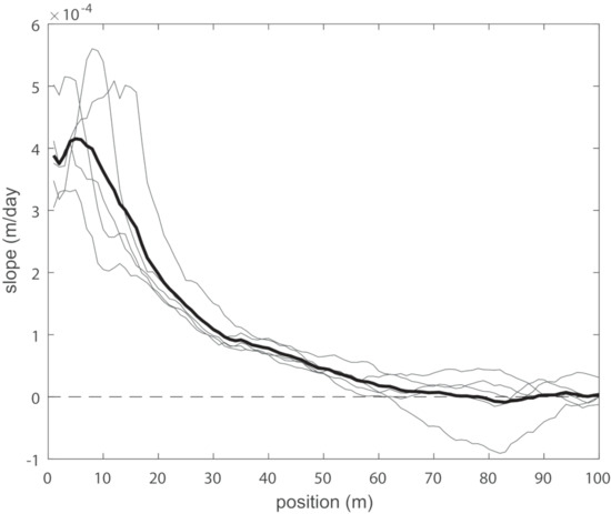
Figure 7.
Estimation of the progradation rate as a function of the position along the Coastal Division profiles. Gray lines correspond to the slopes estimated separately for the five profiles, while thick black line gives the corresponding average slopes.
The progradation rate is maximum at the origin of the profiles and decreases when moving away from the dunes. Consequently, mean slope decreases when moving away from the dune. Sediment transport increases from the intertidal zone to the dune, that propagated seaward over the last decades. This long-term accretion, observed for a long time at the study site [36], is probably the combination of sand supply from the sand banks, the littoral drift and the adjacent nourished beaches [44]. Integrating this progradation rate along the profile yields an average vertical elevation increase of 0.019 m/y. This corresponds to an accumulated sand volume of about 5.7 m/m·y along the profile. The local elevation increase is however close to 0 beyond the first 80 m and varies greatly within these 80 first meters, as seen from Figure 7.
For the subsequent analyses, these average profiles are substracted from the raw elevation measurements in order to obtain zero-mean residual elevations . These are used for assessing the spatial and temporal variability using the spatial and temporal variograms. Beach progradation is accounted for in all subsequent computations that involve distinct time instants, based on the curve of the average progradation rates, as given in Figure 7. Elevations were corrected over time by considering at each location the slope estimated in Figure 7 and by multiplying it by the time that separates sampled profiles. Therefore, the average profiles are corrected in order to account for the progradation that occurs between time instants t and . It is worth noting that all of the subsequent computations were also done by omitting this progradation correction for comparison purposes (results not shown here) and the results were qualitatively identical.
4.2. Spatial and Temporal Variograms
Based on the zero-mean values, the temporal variability of the elevations is determined by estimating the temporal variogram from the five monitoring profiles at the 54 sampling dates. The normalized temporal variogram (i.e., the temporal variogram divided by the total variance ) is presented in Figure 8. The vertical axis represents the fraction of the total variance , which is reached as a function of the time lag between measurements. It can be seen that about 90% of the total variance is reached for days (i.e., 3 years). Thus, elevations measured at the same position on a profile can be considered as uncorrelated for time lag greater than a few years. This fraction of the total variance is about 25% and 65% for measurements separated by a time lag of one month () and one year (), respectively. This fast increase of the dissimilitude between elevations over time is consistent with the fact that the bars and troughs cannot be observed on the average profiles computed over a time span of 19 years. It emphasizes the stochastic nature of the processes driving bar dynamics through time.
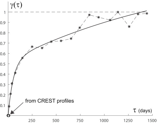
Figure 8.
Estimation of the (normalized) temporal variogram from the Coastal Division profiles (plain circles and dashed line), along with the estimation of the short-range variability obtained from the CREST profiles (white circles). The fitted model corresponds to the thick plain line.
It is not possible to reliably estimate the temporal variogram for any time lag lower than a month due to the fact that monitoring profiles were typically sampled on a monthly basis over the last few years. This estimation can however be done using the campaign profiles sampled daily over short time spans, yielding estimates that match well the general shape of the fitted model (Figure 8). They can also be used to estimate the nugget effect associated with the measurement errors, yielding an estimated value = 7.5 10 m. The corresponding estimated standard deviation m is in close agreement with the reported RMSE of RTK GPS and LiDAR systems, as given in Section 3.1.
While using each monitoring profile for the 54 distinct dates, the spatial variability of the values around the mean profile is assessed by estimating the spatial variogram . As seen in Figure 9, the presence of the bars and troughs is obvious from the periodic behaviour of the variogram. The average distance separating a bar from its neighbouring trough is about 45 m, as measured on this estimated variogram. This means that even if the presence of the bars and troughs cannot be detected on the temporally averaged profiles (Figure 5), these bar systems are, however, present along the profiles. The spatial variogram is not strictly periodic, which emphasizes that the distance between these bars and their amplitude are not constant along the profiles and are also subject to noticeable major fluctuations over time. This is confirmed by the temporal variogram, which shows that elevations are not correlated anymore for time lags longer than few years.
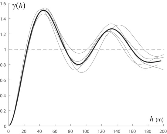
Figure 9.
Estimation of the (normalized) spatial variogram from the five Coastal Division profiles (gray lines), along with the average of these variograms (thick black line). The periodic behaviour of the variogram is associated with the alternance between bars and troughs along the profiles, with an average bar-trough distance of about 45 m.
4.3. Space-Time Model and Volume Changes
From the estimated variance and variogram models and , a ST model as given in Equation (1) is obtained. This ST model can be used in a simulation framework. The beach volume change over time is assessed in order to illustrate the benefits of this space-time modeling approach for our study. The goal is to estimate the displaced volume between two time instant t and , as defined by
where denotes the absolute value and m in our case. The true displaced volumes between two successive sampling dates is first computed for the five monitoring profiles from the measured elevations at the 54 sampling dates. They are compared to the displaced volumes computed while using simulated profiles obtained from Equation (4), to which the prograded volume over the corresponding time span is added. For the five monitoring profiles and the 53 first sampling dates (thus excluding the last date), a large numbers of simulated vectors of elevations at the next sampling time instant are generated conditionally to the observed elevations at time instant t. The predictor of is the average of the volume changes as computed from the various simulated ’s, while using of course the same initial observed elevations in Equation (5). The procedure is illustrated in Figure 10 for the 200 first meters of profile P48 and for a time lag of 34 days. The corresponding volume change values are then computed for each simulation and a distribution of volume change is obtained, from which the average volume change and confidence limits are estimated, as illustrated in Figure 11. The same operation can then be repeated for all profiles and time instants t. The dissimilitude between simulated profiles at time and initial profile at time t increases with , so that the mean volume change and confidence limits increase as well with (Figure 12).
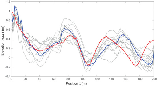
Figure 10.
Illustration of the simulation procedure for profile P48 and a time lag days, where the 10 (out of 10,000) simulated profiles at time instant (gray lines) are all conditioned on the same initial observed values at time instant t (blue line) and where simulated profiles need to be compared to observed values at time (red line). For the sake of readability, only the centered values around the average profile are represented here.
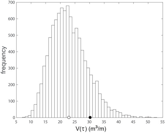
Figure 11.
Distribution of the volume change built from a set of 10,000 simulations, based on the profiles at time instant t and , as given in Figure 10. The open disk is the mean simulated volume change and the black disk is the observed volume change between time instants t and .
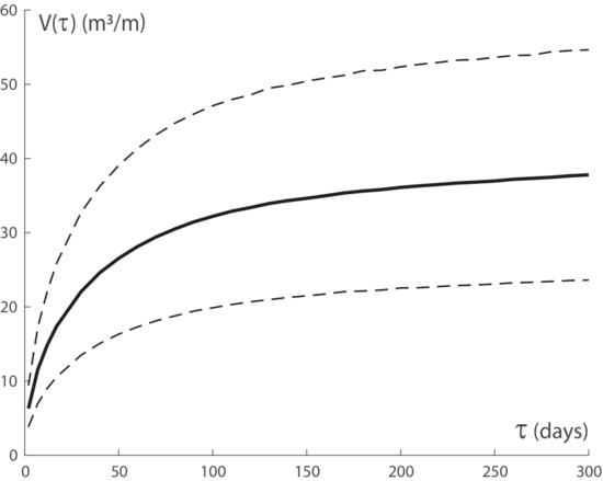
Figure 12.
Mean volume change (plain line) and bounds of the 90% confidence interval of the volume changes (dashed lines) as a function of , as computed here for the 200 first meters of the profile.
The distribution of volume change that was obtained in Figure 11 for days shows that this volume change ranges from 10 m/m to 45 m/m. It is not expected that a single value, like the average volume change (i.e., the mean of this distribution), will closely relate to the true volume change. However, Figure 13 indicates that the true volume changes of each date are in good agreement with those that were obtained from the simulations, except when the true volume changes are higher than 45 m/m (which is typically observed for months). The underestimation of the predicted volume change when the observed volume changes are very high shows here the limitations of the modeling approach. Indeed, Figure 12 shows that the predicted volume change (i.e., mean of simulated volume change distribution) is bounded from above and is not expected to exceed 45 m/m. This is also seen in Figure 13, where predicted volume change only reaches this upper bound when years.
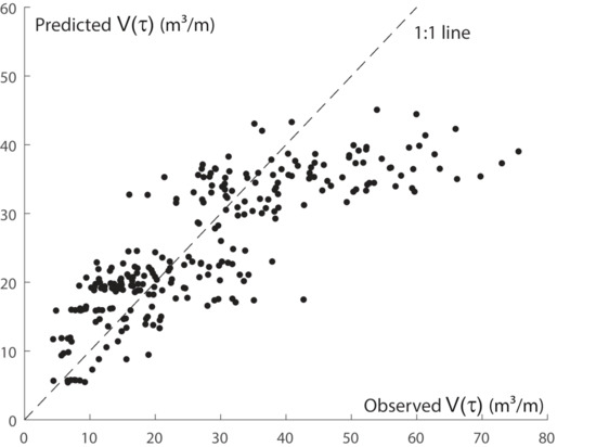
Figure 13.
Comparison of predicted volume changes between time instants t and (i.e., average of the simulated distributions) versus observed volume changes, based on the five Coastal Division profiles at 53 distinct time instants t.
Predicting a volume change for such high time lags is challenging. Firstly, the corresponding profiles at time t and are expected to be poorly correlated (see Figure 8). Secondly, this study is conducted without accounting for the prevailing meteorological and marine conditions that are likely to impact the evolution of the beach between two time instants t and . When increases, so does the probability of observing energetic events, such as storms, which would naturally lead to a higher volume change compared to what would be expected under typical conditions (e.g., [29]). Unfortunately, the effect of meteorological and marine conditions on this study site are still not completely understood. The effective impact of energetic events on volume change is not obvious either, as it depends on various factors (such as wind speed and direction, wave height and energy, etc.) interacting in a nontrivial way.
5. Discussion
5.1. Advantages of this Innovative Model
This study presents an innovative data-driven method for modeling morphodynamics of multi-barred beaches while using high-quality measurements of cross-shore profiles based on a stochastic approach. This is undertaken by first estimating and modeling the spatial and temporal evolution of beach elevations. Subsequently, a separable space-time model is built in order to evaluate the temporal evolution of spatially integrated morphological characteristics. Based on simulations, the temporal evolution of the total displaced sand volume can then be estimated for arbitrary time lags.
A similar stochastic approach could be useful for estimating other beach feature characteristics as long as one is able to capture the stochastic space-time variability of the underlying process. As previously reported [12], the strengths of such stochastic approach are to provide evidence for distinguishing generic characteristics of the data and also that no prior assumptions on the controlling processes are required. The combination of new statistical techniques, the improvement of computer power, as well as increasing length and quality of beach morphology measurements favor the application of a space-time stochastic approach. The findings, specifically the matching of observed and predicted volume changes, also suggest that beach elevation could benefit from being modeled as a stochastic process. Although elevation acts in a non fully predictable way, it can be assessed over both space and time while using a space-time covariance model.
When compared to other approaches, the stochastic method applied in this article provides reliable predictions of barred beach morphology, along with confidence bounds. Other approaches are not usually suited to process intertidal bars. Equilibrium profile models can rarely model intertidal bars. Process-based models still lack the complete understanding of intertidal bar behaviour to accurately process intertidal barred beach morphology (e.g., [45]). In contrast, the method employed to build the model described in this article can be applied to any morphological data set with sufficient measurements or any study site where such measurements can be carried out. Additionally, the model’s poor prediction of long-term large volume change challenges the significance of studies using low measurement frequency (e.g., a survey per year) [46].
5.2. Restrictions of the Model
Regarding the prediction of volume change over time, several improvements need to be considered for further studies. The first one is to include information regarding the prevailing meteorological and marine conditions over a given time interval [t,t+]. These conditions are known to drive morphological change on the beach (e.g., [6,7,47,48]). Energetic events, such as storms, are likely to have a major impact on a beach profile (e.g. [49]). This would thus affect the observed volume change in a way that cannot be predicted by our simple space-time covariance model. Thus, it expected that these volume change predictions would be improved if the effect of these meteorological and marine conditions are accounted for in the simulation procedure. However, in the framework of long-term studies, it is quite unclear how these forcing factors can be easily incorporated in the analysis. Indeed, beach evolution is typically driven by few energetic (erosive) events occurring over few days under stormy conditions, intertwined with long periods of low energetic (recovery) conditions. It is thus unlikely that volume changes as computed from cross-shore profile measurements separated by several months could be related to the largely changing meteo-marine conditions that were acting during that period of time. Additionally, it is worth noting that accounting for meteo-marine conditions this is not even necessarily enough for predicting the evolution, even over short time scales (see, e.g., Biausque and Senechal [25]. Indeed, field observations suggest that alongshore sand displacement driven by tide- and wave- currents might play a role in the intertidal bar morphology. It is already known that sediment transport at this study site has a strong alongshore component [50]. Previous studies found important longshore morphological changes of the bar systems with almost no cross-shore change, under both energetic and calm conditions at another multi-barred macrotidal beach (e.g., in Merlimont, France, [51,52]). The intertidal troughs themselves are also a driver of longshore sediment transport (e.g., [53]). Thus it would be appropriate to undertake a two-dimensional (2D) analysis on both cross-shore and alongshore dimensions, and this analysis should be conducted at a much shorter time scale than for our data sets in order to unambiguously capture the effect of the forcing factors as close as possible to the time of the measurements. Finally, it is worth remembering here that our study focused on the emerged and intertidal zones of the beach, without including the contribution of the submerged area to the volume change assessment. Subtidal bars are likely participate to the dynamics of the intertidal zone. Thus, volume changes that are indicated in this study are subject to revision provided that additional measurements are made available.
5.3. Findings in Bar Morphodynamics
Morphodynamics of beaches with multiple intertidal bar-trough systems have been well documented over the past (e.g., [35,46,47,54,55]). They mainly occur on restricted coasts with a surplus of sand, exposed fetch-limited waves, and large tidal range above 3 m [56]. Previous studies on morphological dynamics of multiple intertidal have reported that the bars tend to be permanent and often appearing at preferential locations [55]. Although intertidal bar are ubiquitous features along the Belgian coast, the findings here indicate that they are subject to major changes over a time span of several years. The temporal and spatial variograms (Figure 7 and Figure 8) suggest no correlation of the position and amplitude of the bars and troughs after three years, with 90% of the total variance reached for days. Thus, a resetting of the intertidal bar profile occurs on annual basis. This is agreement with [57] who found little resemblance of the bars along the Lincolnshire coast (east of England) tracked over time using annual aerial photographs. The morphodynamics of intertidal bar system are principally governed by the tidal range, the incident wave energy level and variability [47]. Bars tend to migrate onshore under calm wave conditions, while they tend to flatten and migrate offshore during storms, with migration rates of up to 10 m per month [58]. However, other factors, such as wave angle and water depth at the bar crest, may force the effect of particular wave conditions on bars development. Additionally, alongshore sediment transport can play an important role on the dynamics of the system, especially in the troughs due to longshore currents over the tidal cycle [7]. The morphological response of the intertidal bars can be affected by relation time effects and morphological feedbacks. The complex and stochastic nature of the processes driving the position and behaviour of the bar-through system are highlighted in the space-time covariance model. Improved knowledge on the development of intertidal bar systems will be beneficial to coastal managers, for whom the evolution of bars is a key component in preventing coastal erosion.
6. Conclusions
To the best of our knowledge, this study is the first to investigate the morphodynamics of sandy multibarred beach that was based on a space-time stochastic approach by relying on a space-time covariance model and a stochastic simulation procedure. It presents a space-time analysis and modeling of cross-shore profiles of a macrotidal beach on the Belgian coast, characterized by intertidal bar systems exhibiting significant changes over time. Often traditional morphodynamic studies characterize the main spatial properties and the temporal evolution of the bars and troughs. However, this article suggests that a stochastic approach is relevant when modeling the temporal evolution of integrated properties along such cross-shore profiles.
The spatial and temporal evolution of beach elevation is estimated and modeled for a set of high-quality measurement profiles over 19 years in order to build up a space-time model. Spatial and a temporal variograms are used in order to quantify the extent of the spatial and temporal dependence of elevation. The findings provide evidence of counter-intuitive facts, such as the absence of bars and troughs on the temporally averaged profiles despite their ubiquitous presence. Based on a space-time separable covariance model, a spatially integrated beach property, like the volume change occurring between two time instants t and , can be assessed through a simulation approach for providing a predicted volume change as a function of , along with corresponding confidence bounds. These findings also suggest that beach elevation could benefit from being modeled as a stochastic process. Besides volume change, other integrated beach morphological characteristics could be predicted in a similar stochastic framework as long as the spatial and temporal evolution of the corresponding processes can be estimated and modeled from the data at hand.
Author Contributions
Conceptualization, P.B.; writing—original draft preparation, P.B.; data analysis, P.B.; data curation, A.-L.M. and M.C.; writing—review and editing, A.-L.M. and M.C. All authors have read and agreed to the published version of the manuscript.
Funding
This research was funded by the Belgian Science Policy Office in the framework of the thematic RS4MODY project (STEREO III project SR/00/360).
Acknowledgments
The authors thank the Coastal Division for providing the RTK-GPS and LiDAR data and Alexis Esquerre for his help in preparing an earlier version of this manuscript.
Conflicts of Interest
The authors declare no conflict of interests.
Data Availability Statement
Research data are not shared.
References
- Cheng, I.; Huang, C.; Hung, P.; Ke, B.Z.; Kuo, C.W.; Fong, C.L. Ten Years of Monitoring the Nesting Ecology of the Green Turtle, Chelonia mydas, on Lanyu (Orchid Island), Taiwan. Zool. Stud. 2009, 48, 83–94. [Google Scholar]
- Sönmez, B. Morphological variations in the green turtle (Chelonia mydas): A field study on an eastern Mediterranean nesting population. Zool. Stud. 2019, 58. [Google Scholar] [CrossRef]
- Boyco, C. New records of sand crabs (Crustacea: Decapoda: Albuneidae and Blepharipodidae) from the western Pacific with description of two new species of Paralbunea Serène, 1977. Zool. Stud. 2019, 59. [Google Scholar] [CrossRef]
- Larson, M.; Capobianco, M.; Jensen, H.; Rozynski, G.; Southgate, H.; Stive, M.; Wijnberg, K.; Hulscher, S. Analysis and modelling of field data on coastal morphological evolution over yearly and decadal time scales. Part 1: Background and linear techniques. J. Coast. Res. 2003, 19, 760–775. [Google Scholar]
- Morton, R.; Paine, J.; Gibeaut, J. Stages and durations of post-storm beach recovery, southeastern Texas coast. J. Coast. Res. 1994, 10, 884–908. [Google Scholar]
- Anthony, E.; Levoy, F.; Monfort, O. Morphodynamics of intertidal bars on a megatidal beach, Merlimont, Northern France. Mar. Geol. 2004, 208, 73–100. [Google Scholar] [CrossRef]
- Masselink, G.; Kroon, A.; Davidson-Arnott, R. Morphodynamics of intertidal bars in wave-dominated coastal settings—A review. Geomorphology 2006, 73, 33–49. [Google Scholar] [CrossRef]
- De Vriend, H.; Capobianco, M.; Chesher, T.; de Swart, H.; Latteux, B.; Stive, M. Approaches to long-term modelling of coastal morphology: A review. Coast. Eng. 1993, 21, 225–269. [Google Scholar] [CrossRef]
- Roelvink, D.; Reniers, A.; Van Dongeren, A.; de Vries, J.; McCall, R.; Lescinski, J. Modelling storm impacts on beaches, dunes and barrier islands. Coast. Eng. 2009, 56, 1133–1152. [Google Scholar] [CrossRef]
- Roelvink, D.; Costas, S. Coupling nearshore and aeolian processes: XBeach and dune process-based models. Environ. Model. Softw. 2019, 115, 98–112. [Google Scholar] [CrossRef]
- Horrillo-Caraballo, J.; Karunarathna, H.; Pan, S.; Reeve, D. Performance of a data-driven technique applied to changes in wave height and its effect on beach response. Water Sci. Eng. 2016, 9, 42–51. [Google Scholar] [CrossRef]
- Southgate, H.; Wijnberg, K.; Larson, M.; Capobianco, M.; Jansen, H. Analysis of field data of coastal morphological evolution over yearly and decadal timescales: Part 2. Non-linear techniques. J. Coast. Res. 2003, 19, 776–789. [Google Scholar]
- Reeve, D.; Horrillo-Caraballo, J.; Magar, V. Statistical analysis and forecasts of long-term sandbank evolution at Great Yarmouth, UK. Estuarine Coast. Shelf Sci. 2008, 79, 387–399. [Google Scholar] [CrossRef]
- Sonu, C.; James, W. A Markov Model for beach profile changes. J. Geophys. Res. 1973, 78, 1462–1471. [Google Scholar] [CrossRef]
- Mason, S.; Hansom, J. A Markov model for beach changes on the holderness coast of England. Earth Surf. Process. Landf. 1989, 14, 731–743. [Google Scholar] [CrossRef]
- Swales, A. Geostatistical Estimation of Short-Term Changes in Beach Morphology and Sand Budget. J. Coast. Res. 2002, 18, 338–351. [Google Scholar]
- Ruessink, B.; Van Enckevort, I.; Kuriyama, Y. Nonlinear principal component analysis of nearshore bathymetry. Mar. Geol. 2004, 203, 185–197. [Google Scholar] [CrossRef]
- Gunawardena, Y.; Ilic, S.; Pinkerton, H.; Romanowicz, R. Nonlinear transfer function modeling of beach morphology at Duck, North Carolina. Coast. Eng. 2008, 56, 46–58. [Google Scholar] [CrossRef][Green Version]
- Pape, L.; Ruessink, B.; Wiering, M.; Turner, I. Neural network modelling of nearshore sandbar behaviour. In Proceedings of the International Joint Conference on Neural Networks ’06, Vancouver, BC, Canada, 16–21 July 2006; pp. 8743–8750. [Google Scholar]
- Yates, M.; Guza, R.; O’Reilly, W. Equilibrium shoreline response: Observations and modeling. J. Geophys. Res. 2009, 114. [Google Scholar] [CrossRef]
- Davidson, M.; Splinter, K.; Turner, I. A simple equilibrium model for predicting shoreline change. Coast. Eng. 2013, 73, 191–202. [Google Scholar] [CrossRef]
- Castelle, B.; Marieu, V.; Bujan, S.; Ferreira, S.; Parisot, J.P.; Capo, S.; Sénéchal, N.; Chouzenoux, T. Equilibrium shoreline modelling of a high-energy meso-macrotidal multiple-barred beach. Mar. Geol. 2014, 347, 85–94. [Google Scholar] [CrossRef]
- Lemos, C.; Floc’h, F.; Yates, M.; Le Dantec, N.; Marieu, V.; Hamon, K.; Delacourt, C. Equilibrium modeling of the beach profile on a macrotidal embayed low tide terrace beach. Ocean Dyn. 2018, 68, 1207–1220. [Google Scholar] [CrossRef]
- Montaño, J.; Coco, G.; Antolínez, J.; Beuzen, T.; Bryan, K.R.; Cagigal, L.; Idier, D. Blind testing of shoreline evolution models. Nat. Sci. Rep. 2020, 10. [Google Scholar] [CrossRef]
- Biausque, M.; Senechal, N. Seasonal morphological response of an open sandy beach to winter wave conditions: The example of Biscarrosse beach, SW France. Geomorphology 2019, 332, 157–169. [Google Scholar] [CrossRef]
- Battiau-Queney, Y.; Billet, J.F.; Chaverot, S.; Lanoy-Ratel, P. Recent shoreline mobility and geomorphologic evolution of macrotidal sandy beaches in the north of France. Mar. Geol. 2003, 194, 31–45. [Google Scholar] [CrossRef]
- Van de Lageweg, W.I.; Bryan, K.; Coco, G.; Ruessink, G. Observations of shoreline—Sandbar coupling on an embayed beach. Mar. Geol. 2013, 344, 101–114. [Google Scholar] [CrossRef]
- Angnuureng, D.; Almar, R.; Senechal, N.; Castelle, B.; Addo, K.A.; Marieu, V.; Ranasinghe, R. Two and three-dimensional shoreline behaviour at a MESO-MACROTIDAL barred beach. J. Coast. Conserv. 2017, 21, 381–392. [Google Scholar] [CrossRef]
- Haerens, P.; Bolle, A.; Trouw, K.; Houthuys, R. Definition of storm thresholds for significant morphological change of the sandy beaches along the Belgian coastline. Geomorphology 2012, 143, 104–117. [Google Scholar] [CrossRef]
- Lebbe, L.; Van Meir, N.; Viaene, P. Potential implications of sea-level rise for Belgium. J. Coast. Res. 2008, 24, 358–366. [Google Scholar] [CrossRef]
- Speybroeck, J.; Bonte, D.; Courtens, W.; Gheskiere, T.; Grootaert, P.; Maelfait, J.P.; Van Landuyt, W. The Belgian sandy beach ecosystem: A review. Mar. Ecol. 2008, 29, 171–185. [Google Scholar] [CrossRef]
- Verwaest, T.; Delgado, R.; Janssens, J.; Reyns, J. Longshore sediment transport along the Belgium coast. In Proceedings of the Coastal Sediments 2011, Miami, FL, USA, 2–6 May 2011; pp. 1528–1538. [Google Scholar]
- MacDonald, N.; O’Connor, B. Influence of Offshore banks on the adjacent coast. In Proceedings of the Coastal Engineering 1994, Kobe, Japan, 23–28 October 1994; pp. 2311–2324. [Google Scholar]
- Afdeling Kust. Getijtafels voor Nieuwpoort, Oostende, Blankenberge, Zeebrugge, Vlissingen, Prosperpolder, Antwerpen en Wintam (Technical Report). In Agentschap Maritieme Dienstverlening en Kust; Vlaamse Overheid: Brussels, Belgium, 2019; Available online: https://www.vlaanderen.be/publicaties (accessed on 25 September 2020).
- King, C.; Williams, W. The formation and movement of sand bars by wave action. Geogr. J. 1949, 113, 70–85. [Google Scholar] [CrossRef]
- Houthuys, R. Morfologische Trend van de Vlaamse Kust in 2011; Technical Report; Agentschap Maritieme dienstverlening en Kust, Afdeling Kust: Oostende, Belgium, 2012; p. 150. (In Dutch) [Google Scholar]
- Akima, H. A new method of interpolation and smooth curve fitting based on local procedures. J. ACM 1970, 17, 589–602. [Google Scholar] [CrossRef]
- Dolan, R.; Fenster, M.; Holme, S. Spatial Analysis of Shoreline Recession and Accretion. J. Coast. Res. 1992, 8, 263–285. [Google Scholar]
- Harley, M.; Turner, I.; Short, A.; Ranasinghe, R. Assessment and integration of conventional, RTK-GPS and image-derived beach survey methods for daily to decadal coastal monitoring. Coast. Eng. 2011, 58, 194–205. [Google Scholar] [CrossRef]
- Cressie, N.; Wikle, C.K. Statistics for Spatio-Temporal Data; Wiley: New-York, NY, USA, 2011; p. 624. [Google Scholar]
- Chun, Y.; Griffith, D.A. Spatial Statistics and Geostatistics: Theory and Applications for Geographic Information Science and Technology; Kwan, M.-P., Ed.; SAGE Advances in Geographic Information Science and Technology Series; University of California: Berkeley, CA, USA, 1993; p. 200. [Google Scholar]
- Jenkins, G.; Watts, D. Spectral Analysis and Its Applications; Emerson-Adams Press: Boca Raton, FL, USA, 2000; p. 525. [Google Scholar]
- Li, Y.; Lark, M.; Reeve, D. Multi-scale variability of beach profiles at Duck: A wavelet analysis. Coast. Eng. 2005, 52, 1133–1153. [Google Scholar] [CrossRef]
- Brand, E. Intertidal Beach Morphodynamics of a Macro-Tidal Sandy Coast (Belgium). Ph.D. Thesis, Vrije Universeit Brussel, Brussel, Belgium, 2019. [Google Scholar]
- Cohn, N.; Hoonhout, B.; Goldstein, E.; De Vries, S.; Moore, L.; Durán Vinent, O.; Ruggiero, P. Exploring Marine and Aeolian Controls on Coastal Foredune Growth Using a Coupled Numerical Model. J. Mar. Sci. Eng. 2019, 7, 13. [Google Scholar] [CrossRef]
- Miles, A.; Ilic, S.; Whyatt, D.; James, M. Characterizing beach intertidal bar systems using multi-annual LiDAR data. Earth Surf. Process. Land. 2019, 44, 1572–1583. [Google Scholar] [CrossRef]
- Kroon, A.; Masselink, G. Morphodynamics of intertidal bar morphology on a macrotidal beach under low-energy wave conditions, North Lincolnshire, England. Mar. Geol. 2002, 190, 591–608. [Google Scholar] [CrossRef]
- Cartier, A.; Héquette, A. The influence of intertidal bar-trough morphology on sediment transport on macrotidal beaches, northern France. Z. Geomorphol. 2013, 57, 325–347. [Google Scholar] [CrossRef]
- Karunarathna, H.; Brown, J.; Chatzirodou, A.; Dissanayake, P.; Wisse, P. Multi-timescale morphological modelling of a dune-fronted sandy beach. Coast. Eng. 2018, 136, 161–171. [Google Scholar] [CrossRef]
- Voulgaris, G.; Simmonds, D.; Michel, D.; Howa, H.; Collins, M.; Huntley, D.A. Measuring and Modelling Sediment Transport on a Macrotidal Ridge and Runnel Beach: An Intercomparison. J. Coast. Res. 1998, 14, 315–330. [Google Scholar]
- Anthony, E.J.; Levoy, F.; Monfort, O.; Degryse-Kulkarni, C. Short-term intertidal bar mobility on a ridge-and-runnel beach, Merlimont, northern France. Earth Surf. Process. Land. 2005, 30, 81–93. [Google Scholar] [CrossRef]
- Sedrati, M.; Anthony, E. Sediment dynamics and morphological change on the upper beach of a multi-barred macrotidal foreshore, and implications for mesoscale shoreline retreat: Wissant Bay, northern France. Z. Geomorphol. Suppl. Issues 2008, 52, 91–106. [Google Scholar] [CrossRef]
- Pedreros, R.; Howa, H.; Michel, D. Application of grain size trend analysis for the determination of sediment transport pathways in intertidal areas. Mar. Geol. 1996, 135, 35–49. [Google Scholar] [CrossRef]
- King, C. Beaches and Coasts; St Martin Press: New York, NY, USA, 1972; p. 570. [Google Scholar]
- Masselink, G.; Anthony, E. Location and height of intertidal bars on macrotidal ridge and runnel beaches. Earth Surf. Process. Land. 2004, 26, 759–774. [Google Scholar] [CrossRef]
- Orford, J.; Wright, P. What’s in a name? Descriptive or genetic implications of ridge and runnel topography. Mar. Geol. 1978, 28, M1–M8. [Google Scholar] [CrossRef]
- Van Houwelingen, S.; Masselink, G.; Bullard, J. Characteristics and dynamics of multiple intertidal bars, north Lincolnshire, England. Earth Surf. Process. Land. 2006, 31, 428–443. [Google Scholar] [CrossRef]
- Van Houwelingen, S.; Masselink, G.; Bullard, J. Dynamics of multiple intertidal bars over semidiurnal and lunar tidal cycles, North Lincolnshire, England. Earth Surf. Process. Land. 2008, 33, 1473–1490. [Google Scholar] [CrossRef]


Publisher’s Note: MDPI stays neutral with regard to jurisdictional claims in published maps and institutional affiliations. |
© 2020 by the authors. Licensee MDPI, Basel, Switzerland. This article is an open access article distributed under the terms and conditions of the Creative Commons Attribution (CC BY) license (http://creativecommons.org/licenses/by/4.0/).