Effect of Variations in Water Level and Wave Steepness on the Robustness of Wave Overtopping Estimation

Abstract

The wave overtopping discharge at coastal defense structures is directly linked to the freeboard height. By means of physical modelling, experiments on wave overtopping volumes at sloped coastal structures are customarily determined for constant water levels and static wave steepness conditions (e.g., specific wave spectrum). These experiments are the basis for the formulation of empirically derived and widely acknowledged wave overtopping estimations for practical design purposes. By analysis and laboratory reproduction of typical features from exemplarily regarded real storm surge time series in German coastal waters, the role of non-stationary water level and wave steepness were analyzed and adjusted in experiments. The robustness of wave overtopping estimation formulae (i.e., the capabilities and limitations of such a static projection of dynamic boundary conditions) are outlined. Therefore, the classic static approach is contrasted with data stemming from tests in which both water level and wave steepness were dynamically altered in representative arrangements. The analysis reveals that mean overtopping discharges for simple sloping structures in an almost deep water environment could be robustly estimated for dynamic water level changes by means of the present design formulae. In contrast, the role of dynamic changes of the wave steepness led to a substantial discrepancy of overtopping volumes by a factor of two. This finding opens new discussion on methodology and criteria design of coastal protection infrastructure under dynamic exposure to storm surges and in lieu of alterations stemming from projected sea level rise.

1. Introduction

The required design freeboard height of a costal defense structure is usually determined by hydraulic model tests. Prediction formulae are also frequently used, which are empirically derived and based on the analysis of data stemming from hydraulic model tests. Standard laboratory routines focus on wave overtopping prediction by means of translating a corresponding static design water level (SWL) in a wave flume or basin. The real non-stationary water levels or changes in wave steepness during storm surges are not mimicked. In addition, natural sea states are simulated in a hydraulic model test by means of idealized prototype conditions [1]. The common standard in wave overtopping prediction are model tests with different constant design water levels and wave characteristics during a single test [2,3]. The objective of the present paper was to derive or develop a more realistic approach in hydraulic model testing, as water levels and wave characteristics are rarely constant in nature. The new approach considers dynamic changes of the SWL and the wave steepness in a hydraulic model tests. The impact on measured wave overtopping volumes of the new method is contrasted to constant boundary conditions. We analyzed to what degree the influence of variations in the SWL and the wave steepness is already covered by existing design formulae [2].

The following subsection provides a background on how to conduct hydraulic model tests according to present state-of-the-art procedures. In addition, the dynamic nature of three natural storm surges is highlighted to provide examples, and the procedure of wave overtopping prediction is briefly described. Section 3 provides additional materials and methods, with a particular focus on the required routine derivation for the presented approach and details of the hydraulic model set-up and instrumentation. In Section 4, the obtained results are shown, separated into the influence of the dynamic SWL and dynamic wave steepness on the mean wave overtopping prediction. The results are discussed in Section 5, and model and scale effects are addressed. Finally, the conclusions are drawn regarding the applicability of the new approach in Section 6, and a discussion of necessary future developments is provided.

2. State of the Art

Experiments in laboratory environments are typically conducted with waves of varying height, steepness, or non-linear characteristics. Subsequently, processes and magnitudes of wave run-up and overtopping on coastal defense structures are investigated for a pre-determined structural exposure time frame. This time frame should consider the duration of the storm surge peak and/or a statistically representative number of individual waves. Collected data are usually normalized over time and the width of the structure’s crown in order to yield a robust design estimate. This estimate is then compared with other modelling approaches or converted to a prototype-scale structure. It is a common standard in laboratory facilities that a typical time series of a representative wave spectrum in a single hydraulic test focusing on wave overtopping should contain at least1000 individual waves, whereas this value by itself is worthy of discussion [4]. A larger number of incident waves (i.e., longer time series in the laboratory facility) allows for a statistically more representative data set [2,5] by means of attenuating the weight of individual extreme waves on run-up and overtopping in the data. Nonetheless, the recommended design parameter of 1000 waves is a kind of artificial commodity in laboratory wave experiments which is capable of representing a typical storm and storm surge of approximately 3 h in the North Sea (e.g., at the German coast).

It is obvious that the $SWL$ during a natural storm surge is always inconstant, yet it is simplified in the present model approximation in laboratory facilities. Astronomical tides, global and local wind fields, meteorologically induced pressure fluctuations, infragravity waves, and swell waves from the north east (NE) Atlantic affect and subsequently alter the near-shore $SWL$—particularly during a storm surge—and lead to an oscillation with corresponding periods from hours to days [6].

The following section provides exemplary field data highlighting the described dynamic characteristic of storm-surge-related water levels and spectral wave conditions. We also briefly describe the common standard in wave overtopping prediction.

Background

Typical dynamical features of the SWL are depicted in Figure 1a by the hydrograph of the gauge “Old Weser Lighthouse” (LAW) in the North Sea in vicinity of the artificially maintained outer estuary of the river Weser [7]. The gauge has a standard elevation zero of NHN16 = −4.96 m and is located about 10 km NE of the German island Wangerooge. The three storms Christian (10/2013), Xaver (12/2013), and Elon (01/2015) were analyzed for reference. These storms represent the three typical types that occur within the North Sea—namely, Jutland (Xaver), Scandinavian (Christian), and Skagerrak (Elon) type events, following different storm tracks. In order to arrive at a more general description of statistical significance, more storm events are required, which must (i) register as a storm surge and (ii) not disrupt the measurement chain, resulting in time series gaps due to destroyed or dislodged buoys. For the years 2009–2019, the three events presented above were the ones that could be observed at this location. The locally gathered non-stationary water level $h_s\left(t\right)$ is presented $\pm 3$ h before and after the maximum peak of the storm surge and normalized by the maximum water level $h_{s,max}$ in Figure 1a. The temporal evolution of the wave steepness (Figure 1b), wave height (Figure 1c) and wave period (Figure 1d) are also given ($dt=60 \mathrm{s}$, corresponding time window for spectral analysis: 15 min).

Obviously, the water level of each individual storm surge varied significantly $\left(\mathsf{\Delta }{h}_s\approx 3.0 \mathrm{m}\right)$, as did the intensity in the analyzed time interval. For all three storm surges, the wave steepness reached its maximum at the peak water level and attenuated with decreasing water level (Figure 1b). Within three hours, the mean wave steepness increased from 0.01 to 0.015. The maximum wave height is reached about 1 h before the storm surge peak water level and is almost constant until the peak water level and decreases afterwards (Figure 1c). During the three hours before the peak water level the wave height increased about 1.0 m for storm Xaver and storm Elon and 2.5 m for storm Christian. The wave period was almost constant for storm Xaver $\left(T_p\approx 7.5 \mathrm{s}\right)$ and storm Elon $\left(T_p\approx 7.5 \mathrm{s}\right)$ whereas for storm Christian the wave period increased significantly from 3 to 2 h before the peak ($4 \mathrm{s}<T_p<7.5 \mathrm{s}$, with a temporary maximum of $T_{p,max}=11.4 \mathrm{s}$) and remained almost constant from that point on. Re-analysis of storm surge characteristics and associated wave conditions for the three selected storms and data at gauge LAW is far from being representative for all locations and storms on the German North Sea coastline. These three examples should raise awareness of the non-stationary quality of typical water levels and wave conditions during storm conditions.

In the following, the influence of dynamic water levels on the wave overtopping prediction is briefly addressed. It is well known that the remaining freeboard height $R_c$ is directly related to the mean wave overtopping discharge $q$. This relation is given by

$$q/\sqrt{g{H}_{m0}^3}=\mathrm{a}\exp \left[-{\left(b{R}_c/H_{m0}\right)}^c\right] \mathrm{for} R_c>0,$$

(1)

where $g$ is the gravitational acceleration and $a$, $b$, and $c$ are empirically derived regression parameters [2]. To calculate the average overtopping discharge on a plain smooth slope ($\cot \alpha >2$), for perpendicular wave attack and breaking waves the parameters are derived from the regression of a large number of hydraulic model tests to $\mathrm{a}= 0.023{ \mathsf{\xi }}_{\mathrm{m}-1,0}/\sqrt{\tan \mathsf{\alpha }})$, $b=2.7$, and $c=1.3$. The definition of the Iribarren number is $\mathsf{\xi }=\tan \alpha /{\left(H/L\right)}^{0.5}$. According to Equation (1), the mean wave overtopping discharge $q$ increases for decreasing freeboard heights $R_c$, respectively increasing water levels, and a decreasing wave steepness. Figure 1 indicates that both quantities fluctuated during a time interval of 3 h ($10,800 s/~7.5 \mathrm{s} \left(T_p\right) \approx 1400$ waves).

The evidently identified dynamical features of SWL and the associated time-varying hydraulic parameters are not represented in any commonly acknowledged hydraulic model test configuration. It is therefore necessary to revisit and understand the underlying processes and elucidate the role of non-stationary water level and wave steepness on the robustness of wave overtopping estimation. The proper adjustment of temporal alterations of design parameters in laboratory facilities is a chief attribute in determining the means and non-stationarity of the determined wave overtopping volumes.

3. Materials and Methods

As many findings regarding wave overtopping are based on hydraulic model tests with a comparable number of waves but a constant characteristic wave steepness and a constant water level, the meaning of this model approximation is discussed in the following. A special set of hydraulic model tests was designed and conducted in a mid-sized laboratory facility. The facility has state-of-the-art wave generation and absorption qualities in order to refer to the initial question as to whether dynamically altered water level changes and varying wave steepness are robustly represented in existing design formulae originating from static configurations in experimental facilities. A detailed description of the facility is provided in Section 3.2. The recorded data allow a quantification of the influence of varying water levels during overtopping design tests of coastal defense structures. This allows an assessment of uncertainties in the present design process.

3.1. Reproduction of Dynamic Changes of Wave Characteristics in Hydraulic Model Tests

The focus of the present study was still on the approximation of nature-like hydraulic boundary conditions in a physical model test. Hence, different scenarios had to be developed in order to cover the dynamic qualities of the hydraulic boundary conditions observed in the prototype time series (Figure 1). They also had to be as simple as possible in order to avoid an overly complex procedure. Therefore, an initial partitioning of the initial time series was undertaken. The whole time series was divided into three subsections (A, B, and C) with equal length (Figure 2a).

In classical hydraulic model tests with a focus on the prediction of wave overtopping, the SWL is kept constant. In this study, the SWL was adjusted during the test following three different approaches: (i) linear increase over the entire test duration, (ii) linear decrease, and (iii) linear increase for the first half followed by a linear decrease in the second half. Configurations (i) and (ii) should physically simulate the lobes of rising and declining water stages prior to and after the maximum water level. Case (iii) encompasses the entire rise and decline time span including the peak water level. A schematic sketch of the three scenarios in contrast with the classical approach of a constant SWL over time $t$ is given in Figure 2a. The integral of the area below these dynamic hydrographs and the constant water level case as data covers the time evolution of the water level changes and its amplitude (Figure 2b). If $A1-A2=0$, the constant water level represents the mean water level over time.

To design an approach for the reproduction of a varying wave steepness over the simulation time span, we followed a procedure analogous to the adaption of the SWL. The main wave characteristics in a time series were defined with the corresponding wave spectrum which defines the magnitude of wave energy density spectrum $S\left(f\right) \left({\mathrm{m}}^2\mathrm{s}\right)$ for each wave frequency $f \left(1/\mathrm{s}\right)$. The frequencies represent the quantity of different wave periods $\left(T = 1/f\right)$ spectrally composing the time series. The wave heights $H$ in the time series of a wave spectrum represent the corresponding wave energy. As the wave period is (dependent on the water depth) directly related to the wave length, the wave steepness $s = H/L$ is also defined by the wave spectrum. Depending on the target of the analysis, a wave spectrum can be analyzed regarding, for example, maximum values (e.g., $H_{max}, T_{max}$), mean values (e.g., $H_m, T_m$), statistical values (e.g.,$H_{1/3}, T_{1/3}$), spectral values (e.g., $H_s,T_p$), weighted values (e.g., $H_{m0}, T_{m-1,0}$), and others. For this study the spectral wave height $H_{m0}$ and the spectral wave period $T_{m-1,0}$ were chosen, as these values are commonly applied when calculating mean overtopping volumes [2]. $H_{m0}$ is derived from the variance of the surface elevation $\eta$ and is calculated to be $H_{m0}=4{\left(m_0\right)}^{0.5}$ from the zeroth spectral moment $m_0$—a characteristic quantity of the spectrum. The spectral wave period is characterized by $T_{m-1,0}=m_{-1}/m_0$ in order to provide a higher weight to the long period parts of the spectrum, as these components more dominantly influence the wave overtopping [2].

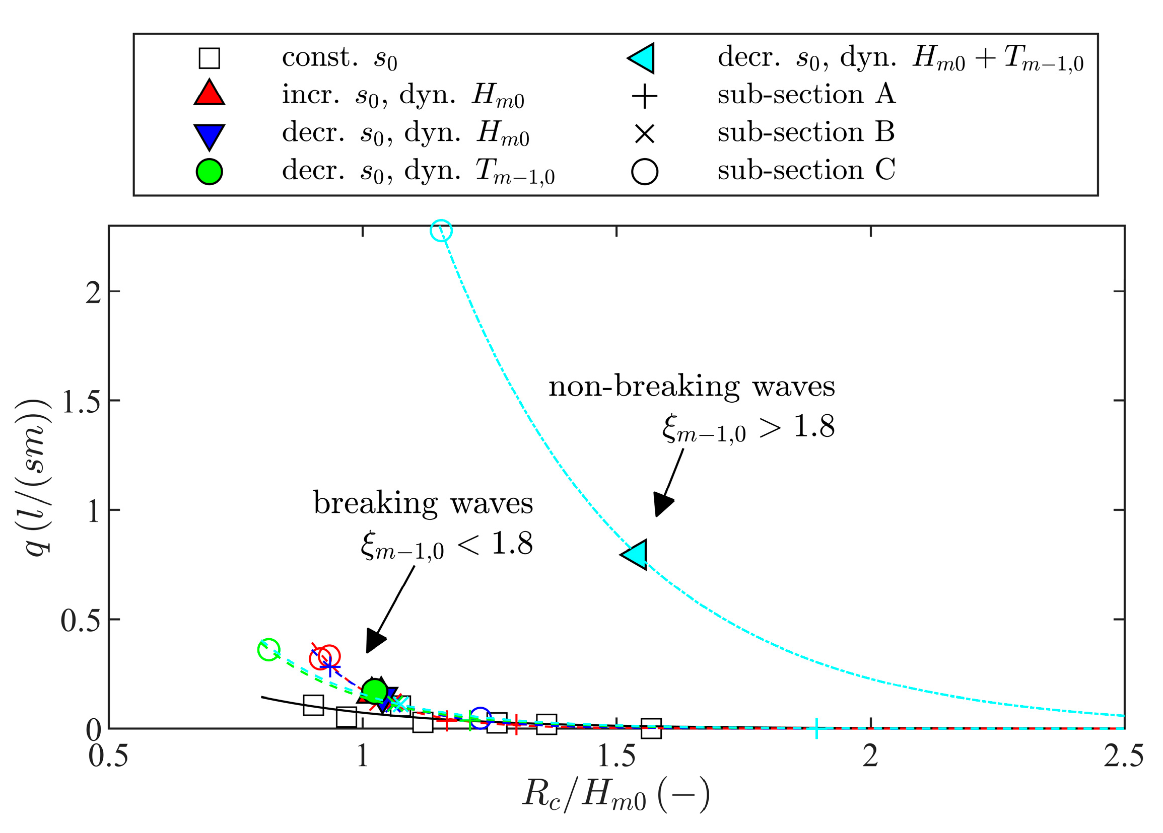
The role of the changing wave steepness on wave run-up and overtopping during the storm surge should address two main characteristics—namely, increasing and decreasing wave steepness during the test—and can be introduced either gradually or in a block-wise configuration in the time series. These characteristics were tested for constant, increasing, and decreasing SWL. Changing wave steepness in a non-stationary pattern can be induced by the variation of either the wave height, the wave period, or an arbitrary variation of both parameters in parallel. The scenarios analyzed in this study are exemplified in Figure 3.

Figure 3a describes the boundary conditions from a classic hydraulic model test with constant boundary conditions in the three subsections A, B, and C. Figure 3b describes the artificially induced increase of the wave steepness by a linearly increasing the wave height while keeping the wave period constant, and Figure 3c represents the induced increase of the wave steepness by means of a block-wise increase of the wave heights in subsections A, B, and C with constant wave period. The linear increase of the wave height in Figure 3b was achieved by a linear amplification of the stroke signal for the piston-type wave maker after a classic calculation of the board motion [1]. A smooth decrease of the wave steepness triggered by a decreasing wave height is depicted in Figure 3d. The most complex scenario is given in Figure 3e. A linearly increasing wave height and a block-wise increasing wave period lead to a gradually decreasing wave steepness. The block-wise increase of the wave period was chosen in order to apply approved spectra-generation routines in each subsection (A, B, and C).

A transient wave steepness evolution scenario (i.e., generation routine in laboratory facilities) for a gradually increasing wave period has not been introduced and analyzed until now, and needs to be implemented in ongoing research. The common methodological approach to the sound reproduction of the wave spectra in each respective subsection was applied to correlate data with existing prediction formulae. Hence, a JONSWAP spectrum with its known characteristics in intermediate and shallow water environments [8] was generated in each subsection. Finally, the three subsections were concatenated into a single time series. Figure 3 shows only a range of different principles enabling dynamic variations of hydraulic boundary conditions. In the present study all combinations of dynamic and constant boundary parameters $\left(H, T, SWL\right)$ among themselves were tested.

With the boundary conditions observed in Figure 1 and the available infrastructure for hydraulic model tests (details in Section 3.2), a model scale of $~1:40$ was chosen. Exemplified time series of different derived surface elevations $\eta$ measured at gauge 5 for corresponding scenarios according to Figure 3 are given in Figure 4.

These scenarios enable the consideration of dynamic changes in the hydraulic boundary conditions in the three defined subsections A (0–333 s), B (333–666 s), and C (666–999 s) of the full time series. The number of waves in a wave spectrum influences the wave overtopping. The length of the subsection of the time series was kept constant during these tests, and therefore the number of waves in each subsection was dependent on the corresponding peak period, and could vary. Within an interval of $333 \mathrm{s}$ in subsections $A$, $B$, or $C$, about 240 waves were generated for the shortest wave period ($T_{m-1,0}=1.39 \mathrm{s}$) and 100 waves for the longest wave period ($T_{m-1,0}=3.34 \mathrm{s}$). It was proven that the standard deviations in measured mean wave overtopping volumes for tests with 125 and 250 waves for a relative freeboard height between 1 and 2 are comparable [4]. Figure 4a shows a classic hydraulic model test with constant SWL and a constant wave steepness $s_0 \left(H_{m0}=0.05 \mathrm{m}, T_{m-1,0}= 2.02 \mathrm{s}\right)$ for the full test time. In Figure 4b, a constant SWL and the block-wise increase of the spectral wave height $\left(H_{m0} \left\{0.05 \mathrm{m}, 0.075 \mathrm{m}, 0.1 \mathrm{m}\right\}\right)$ and constant wave period ($T_{m-1.0}= 2.02 \mathrm{s}$) is given. Figure 4c shows the same boundary conditions as in Figure 4b, but with linearly (smoothly) increasing wave height $(0.05<H_{m0}<0.1)$ over the full time series. Figure 4d shows the same boundary conditions as Figure 4a, with a gradually increasing $SWL \left(\mathsf{\Delta }SWL = 0.025 \mathrm{m}\right)$ over the full test time. A block-wise increase of the spectral wave period $\left(T_{m-1,0} \left\{1.7 \mathrm{s}, 2.0 \mathrm{s}, 2.7 \mathrm{s}\right\}\right)$ and constant SWL and wave height $\left(H_{m0}=0.07 \mathrm{m}\right)$ are given in Figure 4e. In contrast to Figure 4e, the wave height was also block-wise adapted $\left(H_{m0} \left\{0.05 \mathrm{m}, 0.075 \mathrm{m}, 0.1 \mathrm{m}\right\}\right)$ in Figure 4f. Finally, Figure 4g shows the simulation of the peak of a storm surge where the SWL was linearly increased by 0.0125 m in the first half of the test series and decreased analogously in the second half. The wave conditions were constant in this case $\left(H_{m0} = 0.05 \mathrm{m}, T_{m-1,0}= 2.02 \mathrm{s}\right)$. The resulting wave spectra for all scenarios described in Figure 3 measured at the toe of the structure (set-up described in Section 3.2.) are given in Figure 5.

The distribution of the energy density $S\left(f\right)$ is given over the frequency $f$ for different types of sea state evolution for the full time series and the first (A), second (B), and third (C) subsections in Figure 5. Figure 5a gives the measured spectrum from a classic wave generation with constant steepness during the full test. As the full time series consists of three repetitions of the same time series, the spectra in the three subsections and the spectrum of the full time series are almost equal. Minor differences are attributed to side effects of the physical model test (differences in wave reflection over time). Figure 5b shows the spectrum resulting from a decreasing steepness by a linear decrease of the wave height over time. Hence, the spectrum of the first interval had more energy per frequency compared to the second and third intervals. The spectrum corresponding to the full time series shows a somehow average energy distribution from the three subsections. As the peak period $\left(T_p\right)$ did not change for all subsections, the peak frequency $\left(f_p\right)$ was always equal. Results from an increasing wave steepness are given in Figure 5c (block-wise) and 5d (smooth). Although the wave generation differed in both cases, the resulting wave spectra for all subsections and the full time series were almost equal. The effect of a decreasing wave steepness induced by a block-wise increasing wave period and constant wave height is given in Figure 5e. The minimum and maximum spectral peak energy amplitude of all analyzed intervals was close, within a range of factor 2. The peak frequencies differed significantly, as the peak period was also changed in the subsections. While the geometry of the wave spectrum in the three subsections was comparable if the changes of the wave steepness were induced by an adaptation of the wave height, the geometry from subsection to subsection and for the full time series changed obviously by the variation of the wave period over time. Figure 5f shows the spectrum for a decreasing wave steepness induced by a block-wise increasing wave height and a block-wise increasing wave period. As the wave height and wave period were increased in parallel, the total energy increased considerably from subsections A to C. As the total energy of subsection C was dominant, it essentially affected the mean energy distribution for the full time series.

3.2. Model Set-Up and Instrumentation

In order to estimate the influence of a dynamic SWL on the mean overtopping discharge measurement at a coastal defense structure, hydraulic model tests were conducted in a wave flume. The flume was 2.2 m wide and 110 m long. The waves were generated by a piston-type wave maker with 1.8 m stroke, second-order wave generation routines, and active absorption control.

For these specific tests the active absorption control was not used for two reasons: (i) The present wave maker software is not able to consider an active absorption technique with changing $SWL$ over time. To date, there are no standards developed that consider dynamic water level changes over time. (ii) The active absorption technique itself introduces an unknown component (additional wave board motion) to the wave generation process which cannot be controlled actively. Hence, it was decided to permit re-reflections at the wave board. As re-reflections are present in the tests for the classic approach (const. $SWL$ and wave steepness during the test) and the new approach with dynamic variables, the deviations between both tests can be directly attributed to the influence of the dynamic wave characteristics.

The model scale is not relevant for the presented findings, although the boundary conditions were chosen depending on a Froude scale of $1:40$. An impression of the model set-up with instrumentation is given in Figure 6, and a detailed sketch of the model set-up including the position of the instrumentation is given in Figure 7. For these specific tests the flume was separated into two independent reservoirs. Waves were generated in a 25.0-m-long flume section. The adjacent flume section was used as a water storage reservoir and was connected with the test section by a pump system in order to enable dynamic water level changes during the wave generation. The water was pumped behind the tested slope. This area was connected with the remaining test area by a bypass with a height of 0.05 m over the whole flume width of 2.2 m. The maximum in- and outflow velocity from the bypass below the slope was 0.02 m/s. An impact on incident waves was neither visible nor measurable. Overtopping volumes were recorded behind the crest of an idealized $1:6$ sloped dike with a smooth surface for an increasing and decreasing SWL during the tests. For comparison, a reference test series was conducted with constant SWL to allow for correlation analysis with the common guideline [2]. Overtopping volumes from crown exceeding wave run-up were meticulously collected in a box for each subsection (A, B, and C) and their masses were measured continuously during each test. The width of the inlet of the overtopping box was 0.05 m. It is acknowledged that this narrow opening is not optimal, as overtopping volumes always differ in the cross-wave direction along the crest of a structure [9], but this could not be resolved during the present tests.

The surface elevation $\eta$ was measured by ultrasonic wave gauges. Four gauges (gauges 1 to 4) were installed at a distance of 7.7 m from the toe of the slope. At these gauges the incident and reflected wave conditions were determined [10] in order to calculate the reflection coefficient. Gauge 5 was located at the toe of the structure and served as a target boundary condition for post-processing purposes. The calculated wave conditions at this point were corrected regarding the wave reflection determined from the gauge array. Gauge 6 was located close to the interface of SWL and slope.

The water level was varied between $0.74 \mathrm{m} \le h_s \le 0.77 \mathrm{m}$ and represented with the given scale of $1:40$ a maximum storm surge water level difference of about 1.20 m. Increasing and decreasing water levels were controlled in the same range, leading to values for dimensionless SWL changes of $1.6 < H_{m0}/\mathsf{\Delta }{h}_s < 3.3$. Spectral wave heights $H_{m0}$, peak periods $T_p$, and wave steepnesses $s_0 = H_{m0}/L_0$ were varied ($1.0 < R_c/H_{m0} < 2.0$, $0.02 < s_0 < 0.04$) in the tests. The hydraulic boundary conditions analyzed are given in

Table 1. Wave conditions with measured overtopping volumes.

Test Type	Test nr.	Water Level	Wave Height	Wave Period	Iribarren Number	Mean Overtopping Discharge
		${\mathit{h}}_{\mathit{s}}$ (m)	${\mathit{H}}_{\mathit{m}0}$ (m)	${\mathit{T}}_{\mathit{p}}$ (s)	${\mathit{\xi }}_{\mathit{m}-1,0}$ (m)	${\mathit{q}}_{\mathit{A}}$ (L/s/m)	${\mathit{q}}_{\mathit{B}}$ (L/s/m)	${\mathit{q}}_{\mathit{C}}$ (L/s/m)	$\mathit{q}$ (L/s/m)
Const. high SWL	201	0.765	0.050	2.024	1.54	0.053	0.053	0.053	0.053
	202	0.765	0.075	1.723	1.09	0.106	0.106	0.106	0.106
	203	0.765	0.050	1.712	1.35	0.029	0.029	0.029	0.029
Incr. $s_0$	301	0.740	IS	2.038	1.25	0.018	0.124	0.332	0.158
	302	0.740	IS	2.038	1.26	0.035	0.116	0.320	0.157
	303	0.74–0.77	IS	2.038	1.26	0.062	0.226	0.622	0.303
	304	0.77–0.74	IS	2.038	1.26	0.109	0.182	0.339	0.190
Decr. $s_0$	305	0.740	DS	2.038	1.25	0.283	0.109	0.047	0.147
	306	0.74–077	DS	2.038	1.23	0.352	0.191	0.110	0.218
	307	0.77–0.74	DS	2.038	1.23	0.577	0.192	0.054	0.275
Const. low SWL	401	0.740	0.050	2.024	1.60	0.021	0.019	0.019	0.019
	402	0.740	0.075	1.723	1.13	0.027	0.022	0.032	0.027
	403	0.740	0.050	1.712	1.38	0.000	0.000	0.000	0.000
	404	0.740	0.100	1.729	1.00	0.113	0.095	0.101	0.103
Incr. SWL	501	0.74–0.77	0.050	2.024	1.57	0.011	0.017	0.025	0.017
	502	0.74–0.77	0.075	1.723	1.12	0.033	0.051	0.096	0.060
	503	0.74–0.77	0.050	1.712	1.40	0.005	0.013	0.018	0.012
	504	0.74–0.77	0.100	1.729	1.00	0.154	0.207	0.245	0.202
Decr. SWL	601	0.77–0.74	0.050	2.024	1.55	0.035	0.019	0.013	0.023
	602	0.77–0.74	0.075	1.723	1.13	0.104	0.057	0.039	0.066
	603	0.77–0.74	0.050	1.712	1.42	0.016	0.015	0.006	0.012
	604	0.77–0.74	0.100	1.729	1.01	0.294	0.181	0.128	0.201
Decr. s0, const. $H_{m0}$	701	0.740	0.075	DST	1.32	0.037	0.113	0.361	0.171
	702	0.74–0.77	0.075	DST	1.31	0.042	0.059	0.098	0.066
	703	0.77–0.74	0.075	DST	1.32	0.100	0.059	0.039	0.066
	704	0.74–0.77	0.075	DST	1.11	0.051	0.163	0.860	0.358
	705	0.77–0.74	0.075	DST	1.11	0.105	0.169	0.436	0.237
Decr. $s_0$, dyn $H_{m0}$, Tp	801	0.690	IS	DST	1.94	0.000	0.110	2.277	0.796
	802	0.74–0.77	IS	DST	1.78	0.000	0.193	3.850	1.348
	803	0.77–0.74	IS	DST	1.63	0.000	0.128	2.526	0.885
Tidal peak sim.	901	±0.765	0.050	2.024	1.57	0.081	0.106	0.076	0.088
	902	±0.765	0.075	1.723	1.10	0.138	0.172	0.120	0.143
	903	±0.765	0.050	1.712	1.37	0.023	0.029	0.021	0.025
	904	±0.765	0.100	1.729	0.96	0.529	0.491	0.385	0.468
	905	±0.765	0.075	DST	1.32	0.140	0.427	0.995	0.521
	906	±0.765	IS	DST	1.76	0.000	0.429	4.116	1.515
	907	±0.765	DS	DS	1.23	0.792	0.517	0.173	0.494
	908	±0.765	IS	IS	1.25	0.218	0.550	0.743	0.504

IS: $H_{m0,A}=0.05 \mathrm{m}$, $H_{m0,B}=0.075 \mathrm{m}$, $H_{m0,C}=0.1 \mathrm{m}$; DS: $H_{m0,A}=0.1 \mathrm{m}$, $H_{m0,B}=0.075 \mathrm{m}$, $H_{m0,C}=0.05 \mathrm{m}$; DS_T: $T_{m-1,0,A}=1.393 \mathrm{s}$, $T_{m-1,0,B}=2.038 \mathrm{s}$, $T_{m-1,0,C}=3.340 \mathrm{s}$.

and are categorized according to the test type and variation of hydraulic parameters.

4. Results

4.1. Influence of a Dynamic SWL on the Wave Overtopping Prediction

An increasing SWL caused a decrease of the freeboard height $R_c$. The mean wave overtopping discharge $q$ increased with decreasing $R_c$. Figure 8 discloses relative overtopping rates over corresponding breaker-type dependent relative freeboard heights for constant and dynamic SWL changes. Data from the individual subsections of the time series (A, B, and C, defined in Figure 2) are not included for clarity, but showed the same trend. Furthermore, the well-known graph from an empirical prediction [2] including the $5\%$ lower and upper exceedance limits is given for visual correlation of the present data. The spectral wave conditions of the presented data were constant for the whole time series. Only the SWL was dynamically changed during assorted tests $(\#501-\#604$, Table 1.).

The reference data for a constant SWL $(\#201–\#203$, $\#401–\#405$)—representing the classic approach for overtopping prediction in breaking waves (${\mathsf{\xi }}_{m-1,0}<1.7$)—matched the anticipated empirical relation in EurOtop (2018) [2] reasonably well. Deviations between measurements and predictions for the classic approach are attributed to the consciously deactivated active wave absorption during the tests (Section 3.2). It is thus concluded for the present experimental configurations (almost deep water, plain $1:6$ slope) that wave overtopping volumes originating from dynamical water level changes in long time series (>500 waves) were represented robustly. The validity of this statement is attributed to the exponential correlation of freeboard height $R_c$ and overtopping volume $q$. For more shallow water environments (i.e., the intertidal zone Wadden Sea in the southeastern part of the North Sea), the variation of the water depth $h_s$ affects the wave transformation and will inflict stronger influence on the alteration of wave heights and wave periods.

The data show that a constant increase or decrease of the SWL during the test in a range of $1.6 <H_{m0}/\mathsf{\Delta }{h}_s < 3.3$ could be incorporated by the available empirical approach [2] if the mean water level during the full test time $\left(h_{s,mean} = \left(h_{s,start} + h_{s,end}\right)/2\right)$ was applied to the prediction formula. Additionally, the data for dynamic peak simulation and breaking waves fit the prediction following this approach. This means the integral of the area below the hydrograph of the dynamic water level and the mean constant water level as datum applied to the available empirical approach must be equal to zero (Figure 2b). A slightly higher relative overtopping discharge compared to the prediction was measured for nearly non-braking waves $({\mathsf{\xi }}_{m-1,0}=1.4$). As the tests of this study were not repeated several times, we cannot clearly state if this finding is an artefact or a trend.

We conclude that dynamic variations of the SWL during the conduction of a hydraulic model test for prototype durations of about 3 h in a range of $1.6<H_{m0}/\mathsf{\Delta }{h}_s<3.3$ and intermediate water depth ($0.17<h_s/L_{m-1,0}<0.28$) can be incorporated by means of the present design formulae [2] if the mean water level of the analyzed time frame is chosen for the calculation. Therefore, a dynamic variation of the SWL is not required for the prediction of mean overtopping discharges in hydraulic model tests with impermeable, fixed structures and plain slopes in intermediate water depth. However, from a constructional perspective, a dynamic SWL might strongly influence the maximum overtopping of a single wave emerging from the spectrum (important for a rear-slope stability assessment). Consequently, the exerted stress on the structure, the design of filter layers, and the overall stability assessment in classical breakwater studies must be considered [11]. Breaking or broken wave conditions in shallow water were not tested in this study. We assumed that dynamic water levels would significantly influence the energy dissipation during the wave breaking in shallow waters.

4.2. Influence of a Dynamic Wave Steepness s_m−1,0 on the Wave Overtopping Prediction

An increasing wave steepness $s_{m-1,0 }$(decreasing ${\mathsf{\xi }}_{m-1,0}$) led to more intense wave breaking. For plunging waves ($0,2<{\mathsf{\xi }}_{m-1,0}<2-3$) a steep wave front hit the structure or the back, washing water over the slope. For surging waves (${\mathsf{\xi }}_{m-1,0}>2-3$), waves ran up the structure slope without breaking. Plunging waves lost most of their energy by the wave breaking, and surging waves by the interaction with the previous wave run-up and the roughness of the slope. In general, waves break once the ratio of the significant wave height $H_{1/3}$ to the water depth $d_b$ reaches $H_{1/3}/d_b=0.42$. The energy of the incident waves dissipated due to wave breaking is missing for the subsequent wave run-up. Therefore, in general a decreasing overtopping discharge is observed with increasing wave steepness [2]. In the following, the influence of dynamic variation of the wave steepness during a hydraulic model test and a constant SWL on the wave overtopping discharge is discussed.

The measured wave overtopping volume q is given over the dimensionless freeboard height $R_c/H_{m0}$ in Figure 9. For a constant wave steepness, the overtopping volumes were lowest (black squares). For an increasing or decreasing wave steepness induced by a dynamic wave height and a constant wave period during the full time series (red and dark blue triangles), the identified trends were similar. Data measured in subsections A, B, and C are coherent with the data from the full time series.

As the measured wave overtopping volume is given with dimensions over the dimensionless freeboard height, the measured volumes were larger for the tests with increasing and decreasing steepness $(\#301, \#302, \#305$), as this dynamic was triggered by an increasing wave height. Influences of a varying wave steepness were not normalized by this correlation as the wave period was not considered. This is supported by the findings for decreasing wave steepness by a constant wave height and a dynamic wave steepness ($\#701$, green circles). During the first section of the time series (subsection A) the wave steepness was equal with the reference tests for a constant wave steepness. The data points match well with the given trend line for this case. The same is true for the second section of the time series (subsection B). For subsection C, the hydraulic boundary conditions of this test showed the lowest wave steepness. As the largest waves were generated for the simulation of the decreasing wave steepness due to increasing wave height and wave period ($\#801$, light blue triangles) the wave overtopping discharge for this test in subsection C was large and influenced the data points for the full time series significantly.

The classical dimensionless correlation of the relative wave overtopping discharge over the relative freeboard height is given for the present data in Figure 10. The reference data for a constant wave steepness during the full test series ($\#201–\#205$, $\#401–\#405$), representing the classic approach for overtopping prediction in breaking waves $({\mathsf{\xi }}_{m-1,0}< 1.7)$, matched with the prediction line [2]. The deviation from the empirical prediction is again attributed to the consciously deactivated active wave absorption during the tests. A comparability of the findings from the present study with the applied approaches of previous investigations is also given for the assessment of the influence of dynamic wave steepness, as most of the data were covered by the $5\%$ upper exceedance line (representing the $90\%$ confidence band).

Nevertheless, larger dimensionless overtopping rates were measured for all tests with a variation of the wave steepness ($\#301, \#302, \#305, \#701, \#801$). In the case where the wave steepness decrease was triggered by a variation of the wave height and the wave period in parallel, we measured dimensionless wave overtopping volumes that were approximately two times larger compared to the classical approach with constant boundary conditions for the full test time. This finding can be explained by the increased wave reflection $C_r$ for gentler wave steepness and increasing wave breaker parameter ${\xi }_{m-1,0}$ [12]. In test $\#801$, the breaker parameter increased from subsection A (${\xi }_{m-1,0;A}= 1.3; C_r=0.17$) to subsection B (${\xi }_{m-1,0;B}= 1.55;C_r=0.24$) and to subsection C (${\xi }_{m-1,0;C}= 2.2; C_r=0.48$). Hence, the amount of the re-reflected wave energy at the wave maker also increased and led to higher dimensionless wave overtopping rates compared to tests with activated wave reflection compensation according to EurOtop (2018) [2]. In addition, the wave conditions changed from breaking waves (subsections A and B) to non-breaking wave conditions (subsection C).

To quantify the applicability of Equation (1) for the prediction of the overtopping discharge for dynamic hydraulic boundary conditions, the measured overtopping volumes are given over the predicted overtopping volumes in Figure 11. As seen in the previous findings, the dynamic variation of the SWL could be reproduced under the given boundary conditions ($0.05 \mathrm{m} \le H_{m0} \le 0.1 \mathrm{m}$, $1.7 \mathrm{s} < T_{m-1,0} < 3.35 \mathrm{s}$, $0.1 \mathrm{m} < R_c < 0.15 \mathrm{m}$, $1.6 <H_{m0}/\mathsf{\Delta }{h}_s < 3.3$, $0.17<h_s⁄L_{m-1,0} <0.28$). The prediction was valid for the full time series as well as for all three subsections A, B, and C. Measured volumes were at most 0.5 times lower than the predicted ones. The mean accuracy was $q_{meas.}/q_{pred.}= 0.45$ (standard deviation $STD = 0.9$, normalized root mean square error $NRMSE = 0.69$). The prediction of overtopping volumes of a tidal peak simulation ($\#901–\#905$) resulted in only slightly lower values than the measurements. The mean value of accuracy was $q_{meas.}/q_{pred.} = 0.77$ ($STD = 0.98$, $NRMSE = 0.19$). A finer grid of interpolation might improve the prediction. Variations of the wave steepness triggered by a single adaptation of the wave height were on average 2 times over-predicted, and at most 3 times ($\#301–\#307$). Variations of the wave steepness triggered only by an adaptation of the wave period ($\#701–\#705$) showed the most scatter. Hence, the influence of this factor seemed to be over-estimated in the prediction of wave overtopping for a varying wave steepness during the test time. A parallel variation of the wave height and the wave period during the test time ($\#801–\#803$, $\#906–\#908$) amplified the previously discussed scatter and led to a change in the wave-breaking regime from breaking to non-breaking wave conditions. The mean value of accuracy was $q_{meas.}/q_{pred.}= 2$ ($STD = 0.47$, $NRMSE = 0.26$) and therefore the corresponding wave overtopping volume was under-predicted.

5. Discussion

We have shown that the mean overtopping discharge could be calculated for dynamic water level changes with the present literature [2] if the mean water level of corresponding time intervals was used in the formulae. However, this finding is limited to intermediate water depth, which tends to be close to deep water conditions ($0.17<h_s/L_{m-1,0}<0.28$). As the number of waves in a hydraulic model test affects the measured mean wave overtopping volume [4], corresponding variations must be considered in the design of the model tests.

The dynamic variation of the wave steepness led to relevant uncertainties in the prediction of the mean wave overtopping volumes with formulae from the present literature [2]. In addition, it is considered that variations in the wave steepness increase for variations of the SWL over shallow foreshores.

The present findings are plausible expected based on the physical background. Generally, the robustness of the present findings must be proven by further tests with a larger number of variations of time-series of the same spectrum for proof of replication. The quality of results obtained from physical model tests can be improved if active reflection compensation routines allow variations of still-water levels over several minutes. It is estimated that the scatter of the findings can be reduced significantly if these capabilities are incorporated.

The presence of a flat foreshore enabling non-linear wave transformation processes such as shoaling or wave breaking has not been investigated and analyzed in the present experimental configuration. The German Bight is not represented by deep water conditions. Therefore, an additional analysis of the influence of a dynamic SWL in hydraulic model tests for long, shallow foreshores is needed to represent authentic shallow water environments on coastlines and coastal protection structures in the Wadden Sea. For these cases it has already been proven by numerical means that an increasing sea level rise (SLR) results in waves with increased periods and amplitudes due to a reduced influence of the depth-limitation over shallow foreshores [13]. A dynamically increasing SWL induced by a storm surge should cause temporarily comparable boundary conditions as the SLR in long-term. Tide and surge are also affected in addition to the waves, and as a consequence thereof the wave run-up and wave overtopping as well [13]. A 0.5 m change of the SWL leads to an increased required design freeboard height of about $+50\%$. Incidentally, relevant design water levels increase due a non-linear relationship between SLR and changes in extremes [14]. These additional boundary conditions need to be re-considered and studied in a more straightforward experimental configuration.

Furthermore, storm surge characteristics/statistics must be analyzed more profoundly in order to identify the most frequent/substantial trends in the underlying dynamics, as the three exemplarily picked storms and data sets at gauge LAW are far from being representative for all locations and storms on the German North Sea coastline. Accordingly, the present analysis only showcases the principles and effects of the role of a dynamic SWL and a transient wave steepness on the overall wave overtopping. Drivers and interdependencies are not yet fully understood, and strongly call for an extended thorough analysis in order not just to mimic underlying physical processes in laboratory facilities, but also to tailor a safe design of coastal infrastructure under climatic change and sea level rise in the future.

The discussed dynamic hydraulic boundary conditions naturally affect the stability of, for example, breakwater slopes due to variations in the duration and progress of hydraulic loads. As the present set-up focused on influences on mean wave overtopping volumes, a rigid model set-up was chosen. Influences of dynamic water levels on the slope stability of a breakwater are published elsewhere [11].

The present study underlies the known model and scale effects in hydraulic modelling based on the Froude scale, namely, the incorrect reproduction of viscosity, elasticity, surface tension, and others. These parameters affect things such as the wave reflection or wave breaking with less turbulent dissipation during wave breaking. Accordingly, wave overtopping volumes are affected. A thorough discussion of these effects is available in the literature [3]. For the present study, model scale and hydraulic boundary conditions were chosen following approved recommendations for physical modelling and experimentation [3,5].

6. Conclusions

For the first time, this work showcases the principles and effects of the role of a dynamic SWL and a transient wave steepness on the overall wave overtopping. The new approach to considering dynamic changes of the SWL and the wave steepness in hydraulic model tests focusing on the wave overtopping showed that the influence of a variation of the SWL is already covered with the existing design formulae. Yet, investigations on the role of dynamic wave steepness on wave overtopping in hydraulic model tests indicate uncertainties. Present design formulae are not able to cover these effects. This led to errors in the predictions of overtopping volumes with a factor of two in specific cases. These findings are limited to the tested boundary conditions (intermediate water depth, no foreshore influences).

Future investigations should address the effects in shallow water conditions. Adjustments of present wave generation routines and techniques are required to enable active reflection compensation for dynamic water levels during a test. The scientific community has to agree on standardized characterizations/definitions regarding this dynamic procedure in order to enable comparability between facilities.

References

1. Goda, Y. Random Seas and Design of Maritime Structures, 3rd ed.; Advanced Series on Ocean Engineering; World Scientific Publ: Singapore, 2010; Volume 33, ISBN 978-981-4282-40-6. [Google Scholar]
2. EurOtop. Manual on Wave Overtopping of Sea Defences and Related Structures. An Overtopping Manual Largely Based on European Research, but for Worldwide Application, 2nd ed.; Van der Meer, J.W., Allsop, N.W.H., Bruce, T., De Rouck, J., Kortenhaus, A., Pullen, T., Schüttrumpf, H.F.R., Troch, P., Zanuttigh, B., Eds.; 2018; Available online: www.overtopping-manual.com (accessed on 15 October 2019).
3. Hughes, S.A. Physical Models and Laboratory Techniques in Coastal Engineering; World Scientific: Singapore, 1993; ISBN 978-981-02-1541-5. [Google Scholar]
4. Daemrich, K.-F.; Mai, S.; Kerpen, N.B. On the reasons of scatter in data for design formula evolution. In Proceedings of the 6th CG Joint Symposium on Hydraulic and Ocean Engineering, Keelung, Taiwan, 23–29 September 2012; p. 6. [Google Scholar]
5. Frostick, L.E.; McLelland, S.J.; Mercer, T.G. Users Guide to Physical Modelling and Experimentation: Experience of the HYDRALAB Network, 1st ed.; CRC Press/Balkema: Leiden, The Netherlands, 2011; ISBN 978-0-415-60912-8. [Google Scholar]
6. EAK. Empfehlungen für die Ausführung von Küstenschutzwerken; Die Küste; Ausschuss für Küstenschutzwerke: Heide, Germany, 2007; Volume 65, ISBN 978-3-8042-1056-1. [Google Scholar]
7. Waterways and Ship Office (WSA). Bremerhaven Records of Windspeed and Direction, Water Level and Seastate at the Observation Station Lighthouse Old Weser; Waterways and Ship Office (WSA): Bremerhaven, Germany, 2018. [Google Scholar]
8. Hasselmann, K.; Barnett, T.P.; Bouws, E.; Carlson, H.; Cartwright, D.E.; Enke, K.; Ewing, J.A.; Gienapp, H.; Hasselmann, D.E.; Kruseman, P.; et al. Measurements of Wind-Wave Growth and Swell Decay during the Joint North Sea Wave Project (JONSWAP); Deutches Hydrographisches Institut: Hamburg, Germany, 1973.
9. Kerpen, N.B.; Schlurmann, T. Scattering of the Mean Overtopping Discharge along a Crest at Dykes with Topped Vertical Wall. In From Sea to Shore? Meeting the Challenges of the Sea; ICE Publishing: Edinburgh, UK, 2014; Volume 1–2, pp. 1336–1345. ISBN 978-0-7277-5975-7. [Google Scholar]
10. Frigaard, P.; Andersen, T.L. Analysis of Waves: Technical Documentation for WaveLab 3; DCE Lecture Notes; Department of Civil Engineering, Aalborg University: Aalborg, Denmark, 2014. [Google Scholar]
11. Van Gent, M.R.A.; Zwanenburg, S.A.A.; Kramer, J. Effects of water level variations on the stability of rock armoured slopes. Coast. Eng. Proc. 2018, 1, 44. [Google Scholar] [CrossRef] [Green Version]
12. Battjes, J.A. Surf Similarity. In Proceedings of the 14th ASCE Coastal Engineering Conference, Copenhagen, Denmark, 24–28 June 1974; pp. 446–480. [Google Scholar]
13. Arns, A.; Dangendorf, S.; Jensen, J.; Talke, S.; Bender, J.; Pattiaratchi, C. Sea-level rise induced amplification of coastal protection design heights. Sci. Rep. 2017, 7, 40171. [Google Scholar] [CrossRef] [PubMed]
14. Arns, A.; Wahl, T.; Dangendorf, S.; Jensen, J. The impact of sea level rise on storm surge water levels in the northern part of the German Bight. Coast. Eng. 2015, 96, 118–131. [Google Scholar] [CrossRef]
Figure 1. Non-stationary characteristics of storms Christian (10/2013), Xaver (12/2013), and Elon (01/2015) measured at gauge “Old Weser Lighthouse” [7] (estuary of the river Weser in the German bight) ±3 h before and after the maximum peak of the storm surge with a discretization of 60 measured data points per hour. Time series of (a) water level h s ( t ) / h s , m a x , (b) wave steepness H s ( t ) / L p ( t ) , (c) wave height H s ( t ) , (d) wave period T p ( t ) .
Jmse 08 00063 g001
Figure 2. (a) Idealized scenarios to consider dynamical changes in the static design water level (SWL) in the three defined subsections A, B, and C of the full time series. (b) Definition of integrals A 1 and A 2 between the dynamic hydrograph and a chosen constant water level.
Jmse 08 00063 g002
Figure 3. Scenarios to consider dynamic changes in the hydraulic boundary conditions in the three defined subsections of the full time series.
Jmse 08 00063 g003
Figure 4. Time-series of the surface elevation η measured at gauge 5 for corresponding scenarios according to Figure 3 to consider dynamic changes in the hydraulic boundary conditions in the three defined subsections A (0–333 s), B (333–666 s), and C (666–999 s) of the full time series.
Jmse 08 00063 g004
Figure 5. Energy density spectra for different types of sea state evolution for the whole time series and the first (A), second (B), and third (C) subsections. (a) Classic wave generation with constant steepness during the full test; (b) Decreasing steepness by linear decrease of the wave height; (c) Increasing steepness by block-wise increase of the wave height; (d) Increasing steepness by smooth increase of the wave height; (e) Decreasing steepness by increasing wave period and constant wave height; (f) Decreasing steepness by increasing wave height and wave period.
Jmse 08 00063 g005
Figure 6. Impression of the model set-up with instrumentation during test #402.
Jmse 08 00063 g006
Figure 7. Model set-up in a 2D wave flume with position of the instrumentation (measurements in meters) and detail of the beach section.
Jmse 08 00063 g007
Figure 8. Relative wave overtopping data for breaking waves over the breaker-type dependent relative freeboard height for dynamic SWL changes and comparison to EurOtop (2018) [2] with 5 % lower and upper exceedance.
Jmse 08 00063 g008
Figure 9. Relative wave overtopping volume over dimensionless freeboard height for the full time series (filled marker) and values calculated for each subsection A, B, and C (Figure 2) including corresponding exponential trends.
Jmse 08 00063 g009
Figure 10. Wave overtopping data for relative overtopping rate over the relative freeboard height for dynamic wave steepness changes and comparison to EurOtop (2018) [2] with 5 % lower and upper exceedance lines (or 90 % confidence band). (a) Breaking-wave conditions; (b) Non-breaking-wave conditions.
Jmse 08 00063 g010
Figure 11. Measured wave overtopping volumes q m e a s . over predicted overtopping volumes q p r e d . for 0.05 m H m 0 0.1 m , 1.7 s   <   T m 1 , 0   <   3.35 s , 0.1 m   <   R c   <   0.15 m .
Jmse 08 00063 g011