Capacity Analysis for Approach Channels Shared by LNG Carriers


Abstract
:1. Introduction
1.1. Background
1.2. Literature Review
- (1)
- Traffic Capacity Analysis.
- (2)
- LNG Carriers.
1.3. Contributions
1.4. Organization
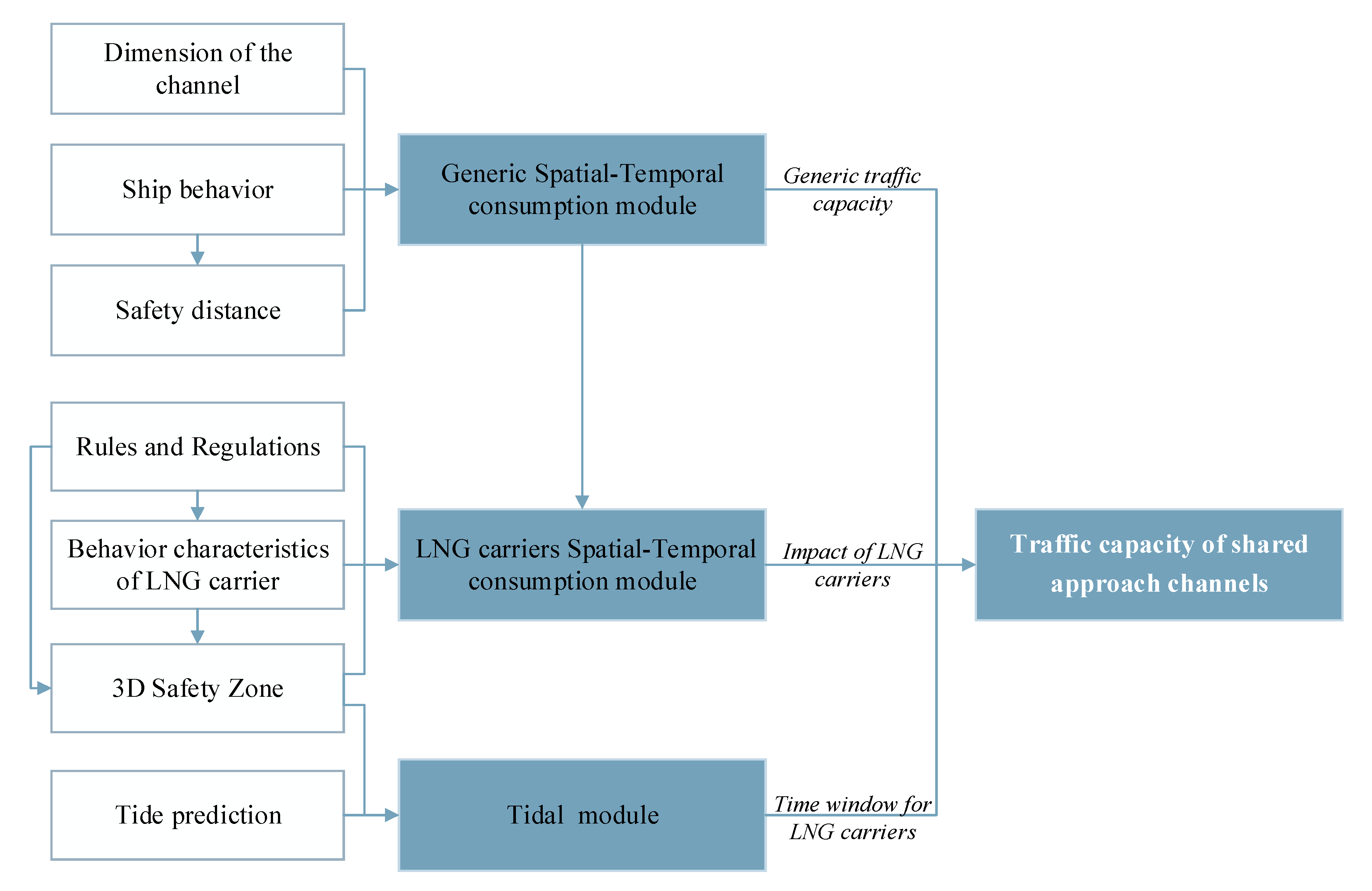
2. Methodology
- (1)
- The Generic Spatial–Temporal Consumption Module.
- (2)
- The LNG Carrier Navigation Module.
- (3)
- The Tidal Module.
3. Capacity Analysis for Shared Approach Channels
3.1. Assumptions
- The OTS navigating in the channel are treated as having the same dimension and the same maneuverability.
- The anchorage and berths are always available. Ships can find some areas to wait ahead of LNG carriers entering or departing the port.
- Meteorological conditions are appropriate for navigation.
- Navigation facilities on the channel are in good condition and provide sufficient supports.
3.2. Generic Spatial–Temporal Consumption Module
3.2.1. Spatial–Temporal Consumption Model
3.2.2. The Impact of Ship Behaviors
3.3. The LNG Carrier Navigation Module
3.3.1. Characteristics of Behaviors of LNG Carriers
- (1)
- When the LNG carrier navigates in shared approach channels, OTS, whose courses are opposite to the LNG carrier, are forbidden to enter the channel. OTS should leave the channel before the LNG carrier inbound.
- (2)
- Some ships are allowed to navigate in the long-distance approach channel. The premise is that the LNG carriers have the priority of the navigation, and OTS should leave enough space and time for the LNG carrier.
- (3)
- OTS and LNG carriers can navigate in the same channel under the traffic control, but the LNG carrier should be equipped with escort ships and tugs.
- (4)
- Authorities should set the proper mobile safety zone for LNG carriers when approaching the channel.
- (5)
- The LNG carrier should enter the port in the daytime.
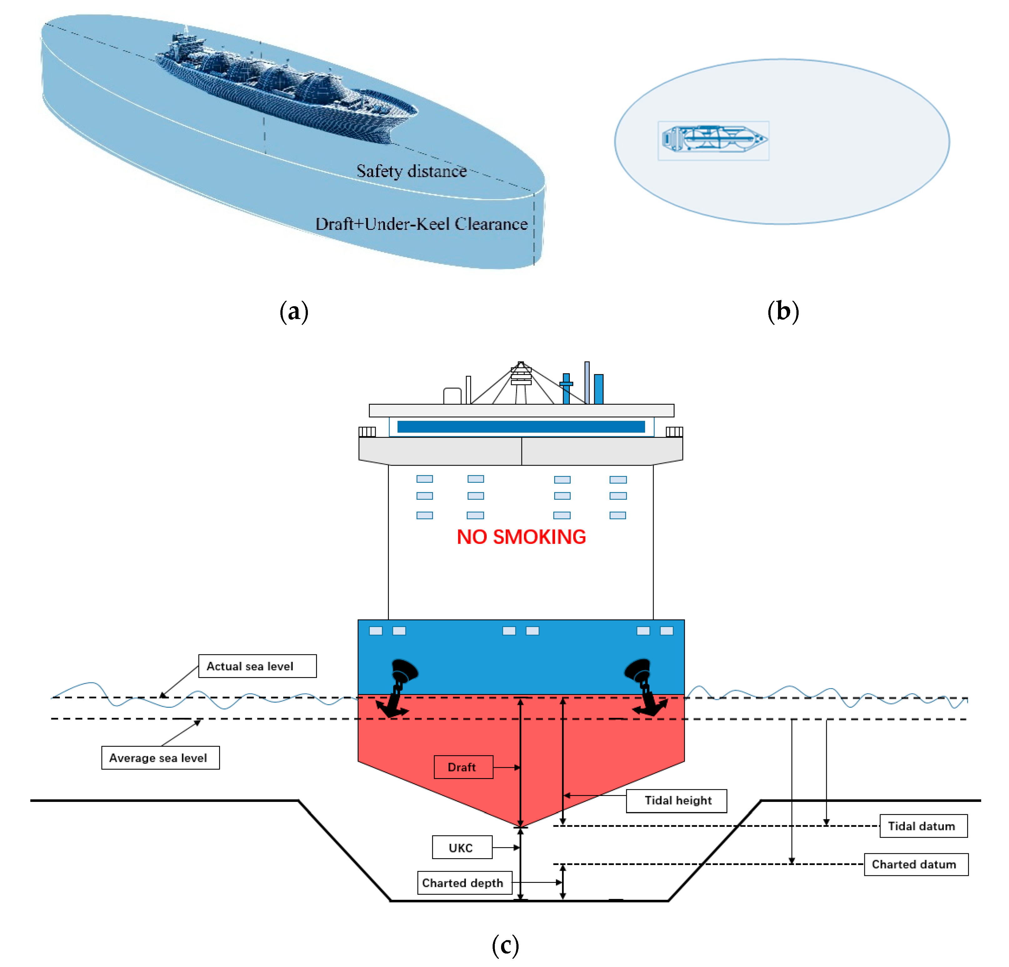
3.3.2. The 3D Mobile Safety Zones for LNG Carriers
- (1)
- Safety Distance.
- (2)
- Under Keel Clearance.
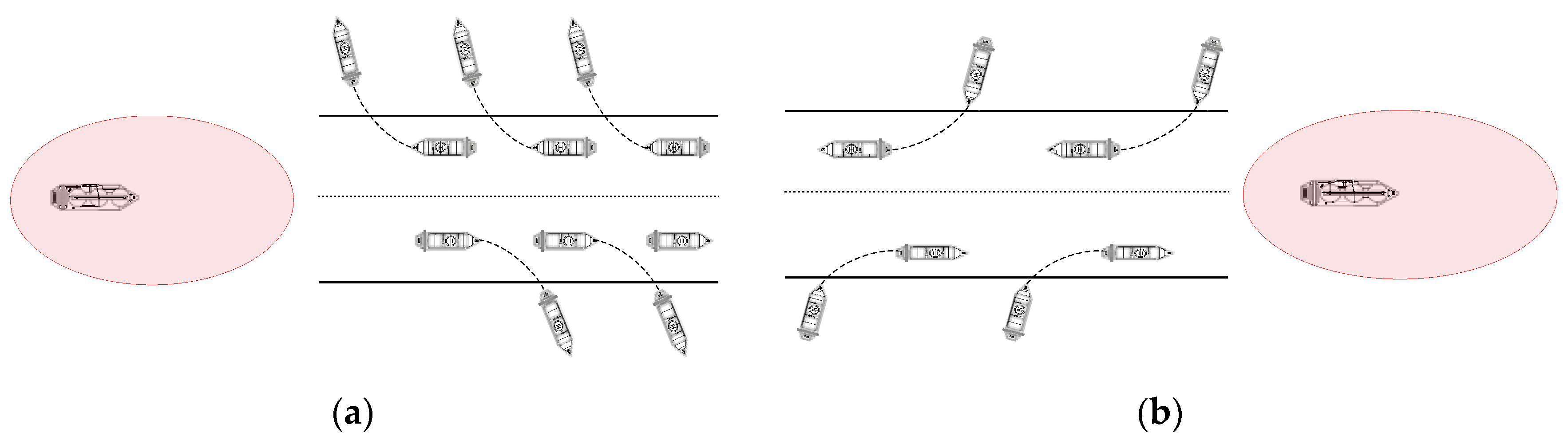
3.3.3. Spatial–Temporal Consumptions of LNG Carriers
- (1)
- Clear the channel. OTS are compelled to leave the channel and wait in the anchorage or the berth before the front edge of the mobile safety zone approaching the entrance of the channel.
- (2)
- LNG carriers pass through the channel. The LNG carriers proceed into the channel at the safe speed with enough tugs, patrol boats, or even the empirical pilots on board. OTS that meet the related requirements can follow the LNG carrier.
- (3)
- Restore the channel order. When the back edge of the LNG carriers’ mobile safety zone leaving the channel sideline, the blocked ships can enter the proper channel. The traffic flow will continue like ever.
3.4. The Tide Module
3.4.1. Tide Prediction
3.4.2. Determination of the Time Windows for LNG Carriers
3.5. The Integrated Module
3.5.1. Steps of Calculation
- (1)
- Calculating the Tidal Time and Tidal Level.
- (2)
- The Total Spatial–Temporal Resources of the Channel.
- (3)
- The Influences Caused by the Inbound and Outbound Ship Behaviors.
- (4)
- The Occupied Spatial–Temporal Resources of LNG Carriers Navigation.
- (5)
- Get the Loss of the Spatial–Temporal Resources.
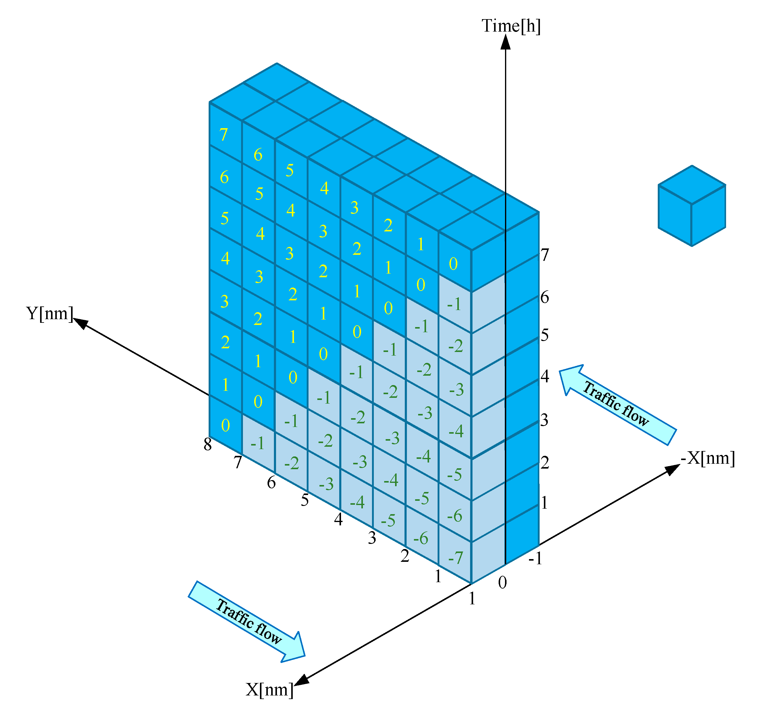
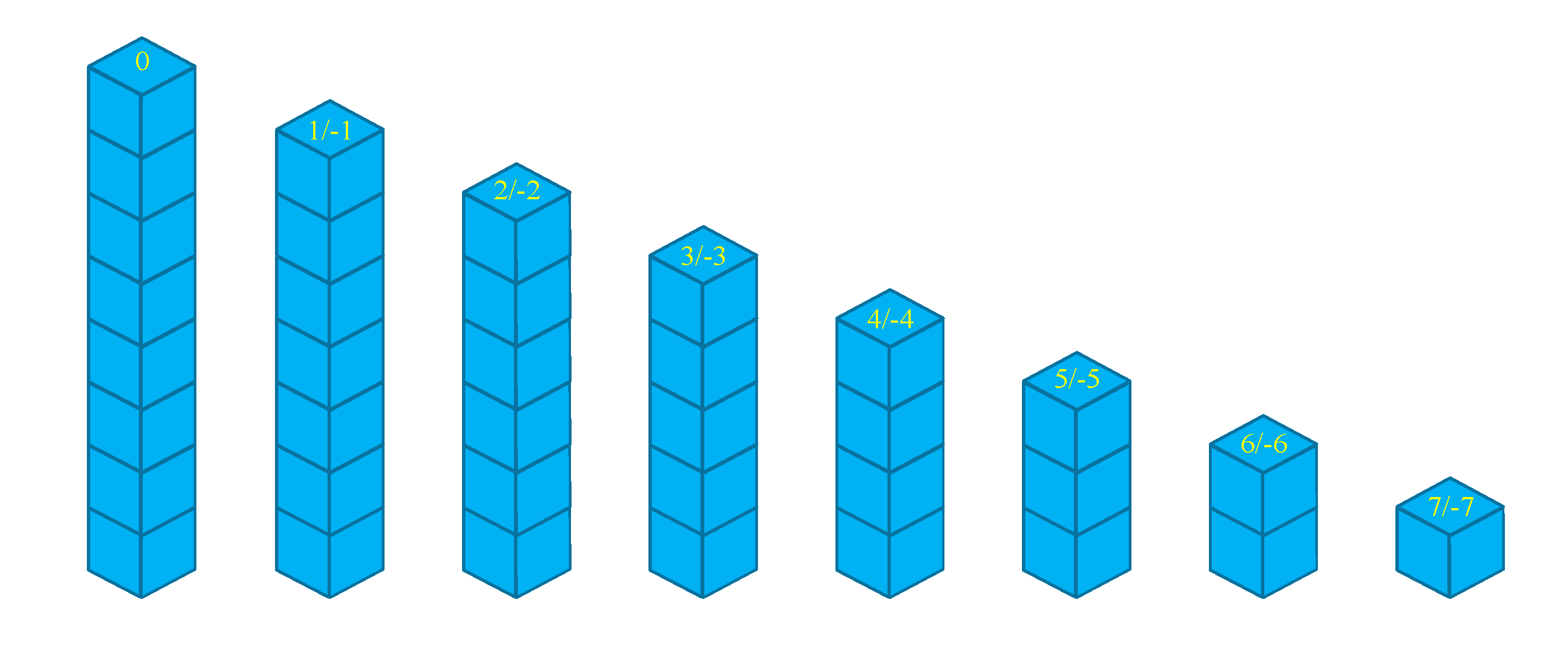
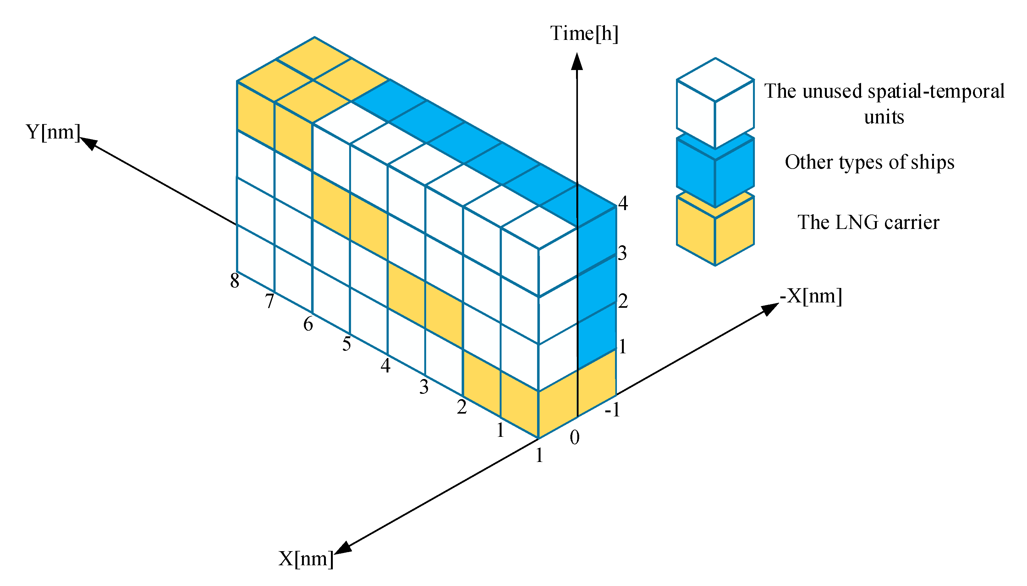
3.5.2. Spatial–Temporal Indexed Chart
- (1)
- Show the Process of Ships Navigation.
- (2)
- The Total Used Spatial–Temporal Resources by the Individual Ship.
- (3)
- The Maximum Number of Ships.
4. Case Study
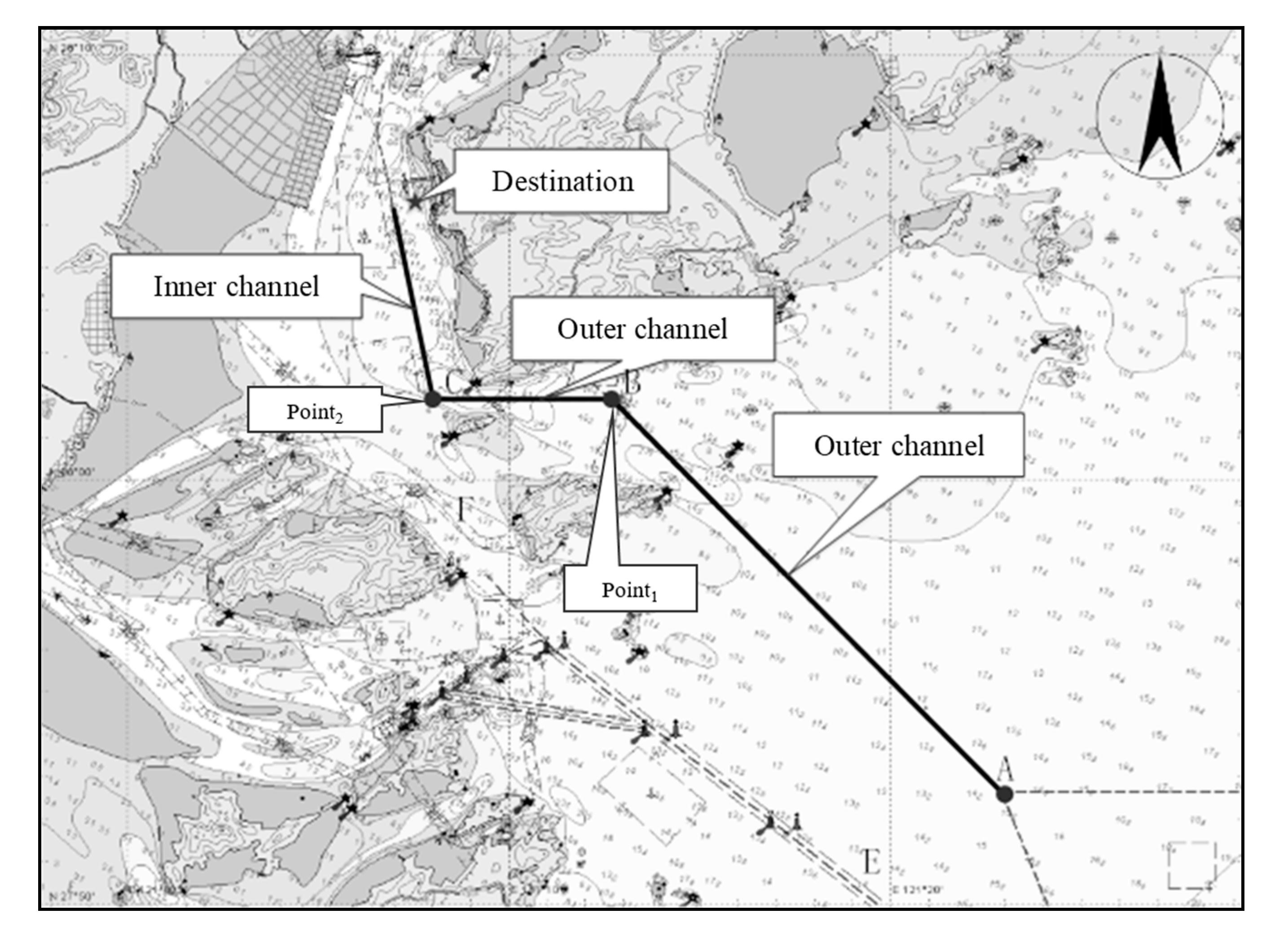
4.1. Setup
- (1)
- Approach Channel.
- (2)
- Tidal Data.
- (3)
- Representative Ships.
4.2. Traffic Capacity of the Approach Channel
4.3. Sensitivity Analysis
4.3.1. Impact of the Size of the Mobile Safety Zones
4.3.2. Impact of Arrival Rate
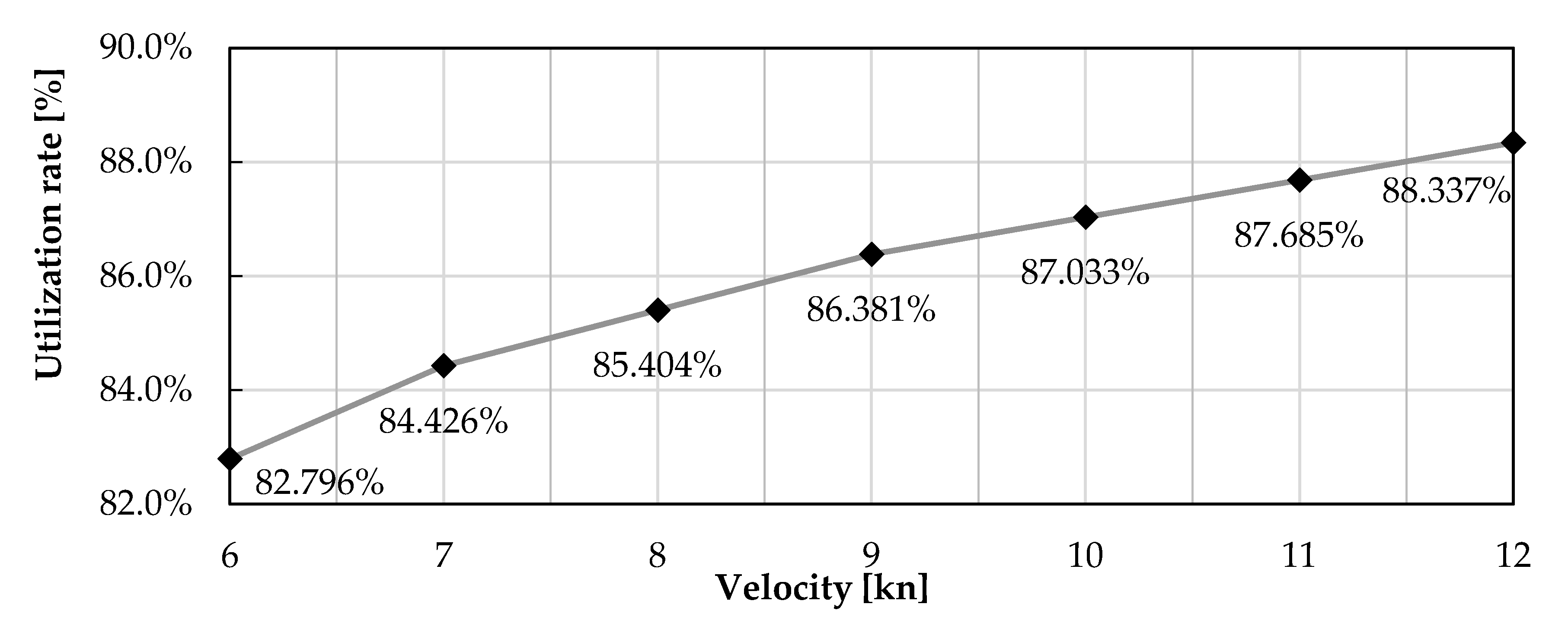
4.3.3. Impact of Velocity
- (1)
- Constant Velocity
- (2)
- Changing Velocity
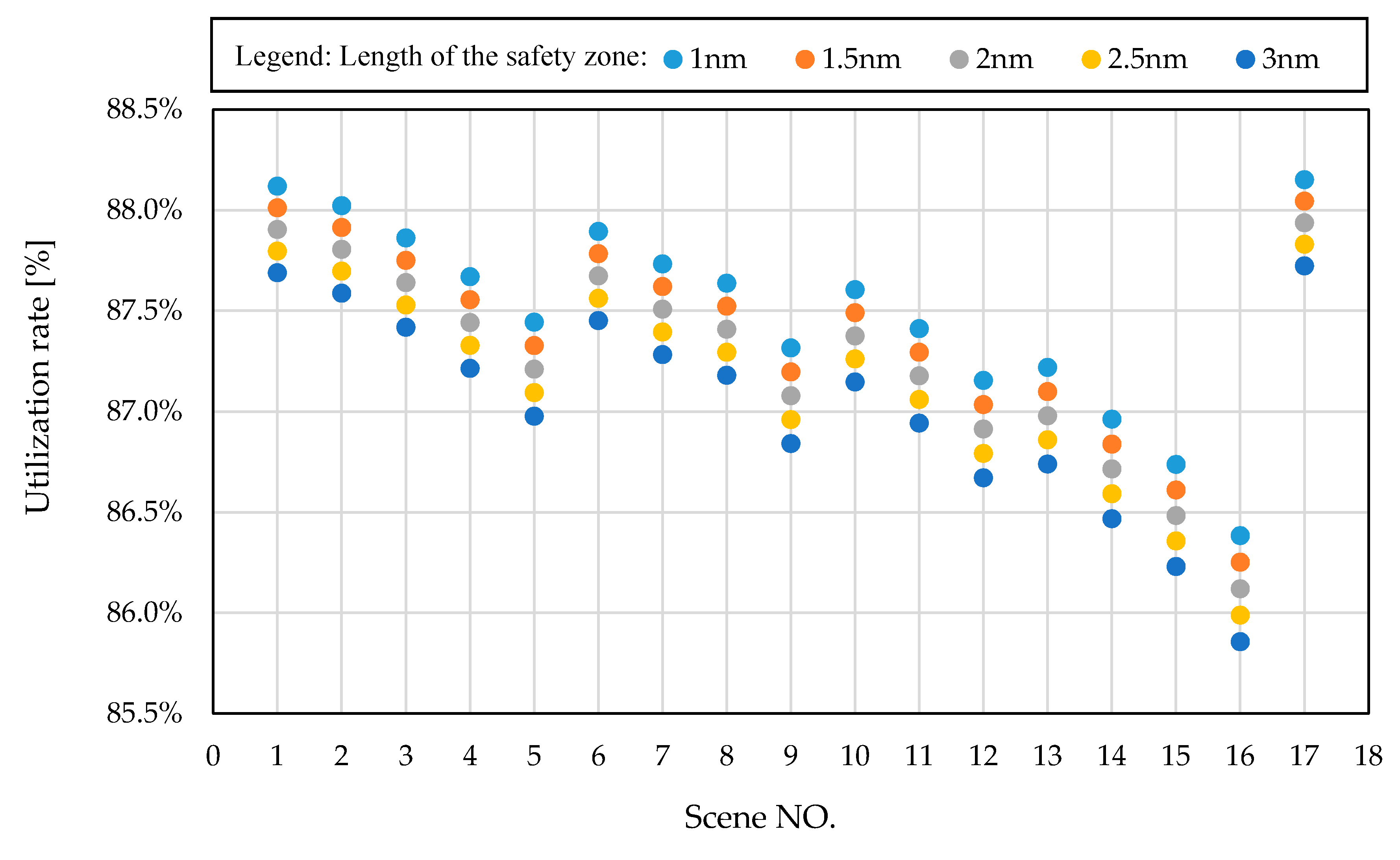
4.3.4. Comparison of Different Traffic Management Strategies
4.4. Discussion
5. Conclusions
- If the arrival rate of the LNG carrier reaches a critical value, which is the maximum number of LNG carriers, OTS cannot use the channel during the tide window. Then the authority could plan to build a special channel to separate the LNG carriers and OTS.
- The utilization rates of the shared channel are affected more by the mobile safety zone than the change of the velocity. Thus, the authorities can improve the utilization rate of the channel by control the size of the mobile safety zone and design an optimal velocity changing pattern.
- However, smaller safety zone and higher speed of LNG carriers may increase the navigation risk. Therefore, balancing efficiency and safety is a significant factor that needs to be considered when making traffic management strategies.
Author Contributions
Funding
Conflicts of Interest
Appendix A

| Symbol | Variables | Symbol | Variables |
|---|---|---|---|
| UKC | Under keel Clearance | , | The period that a ship navigates in the channel |
| Draft | Safety distance between the consecutive ships | ||
| () | Height of the tide | The track zone width of the individual ship. | |
| () | the charted depth | Workable time of the channel in a single day | |
| () | Tidal datum | Average time that a ship used in | |
| () | Chart datum | Crash-stop distance of the later ship | |
| () | Ship squat | Distance in reacting time | |
| () | Water level measuring error | Static safety distance | |
| () | Ship swaying increment | Crash-stop distance of the former ship | |
| () | Relative depth | Length of the former ship | |
| Real depth | Velocity of the later ship | ||
| Length between perpendiculars | Reaction time | ||
| Block coefficients of ship | Plane area of the inbound ship domain | ||
| The depth of the channel | Inbound time | ||
| Molded breadth | Length of the inbound ship | ||
| Ship displacement | Velocity of the inbound ship | ||
| Froude number of ship length | Inbound distance | ||
| Froude number of channel depth | Average velocity of the ships navigated in the channel | ||
| Ship velocity | Safety distance | ||
| Gravity | Length of longitudinal direction | ||
| () | Tidal height | Width in the transverse direction | |
| , | The height and duration of high water | Navigation plane area of the safety zone | |
| , | The height and duration of low water | Navigation time of LNG carriers | |
| Tidal range | Spatial–temporal resources of LNG | ||
| Traffic capacity | Suspension of the spatial–temporal resources | ||
| Total spatial–temporal resources | Used spatial–temporal resources by other types of ships | ||
| , | Time period | Occupied spatial–temporal resources by LNG carriers | |
| Overall length of the channel | Unused spatial–temporal resources in the time of LNG carrier’s navigation | ||
| The maximum available width of channel | Loss of spatial–temporal resources | ||
| The number of the passageway in the channel | Loss rate of spatial–temporal resources | ||
| Resource that the individual ship occupied | Loss number of other types of ships |
References
- Wang, W.; Peng, Y.; Tian, Q.; Song, X. Key influencing factors on improving the waterway through capacity of coastal ports. Ocean Eng. 2017, 137, 382–393. [Google Scholar] [CrossRef]
- International Energy Agency. World Energy Outlook 2019; Organisation for Economic Co-Operation and Development (OECD): Paris, France, 2019. [Google Scholar]
- Liu, K.; Xin, X.; Ma, J.; Zhang, J.; Yu, Q. Sensitivity analysis of ship traffic in restricted two-way waterways considering the impact of LNG carriers. Ocean Eng. 2019, 192, 106556. [Google Scholar] [CrossRef]
- Olba, X.B.; Daamen, W.; Vellinga, T.; Hoogendoorn, S.P. Capacity Estimation Method of a Waterway Intersection. In Traffic and Granular Flow ’15; Springer Science and Business Media LLC: Berlin/Heidelberg, Germany, 2016; Volume 1920, pp. 613–620. [Google Scholar]
- Wei, Z. Calculation model of inland waterway transit capacity based on ship-following theory. J. Traffic Transp. Eng. 2009, 9, 83–87. [Google Scholar]
- Zhang, X.; Mou, J.; Zhu, J.; Chen, P.; Liu, R. (Rachel) Capacity Analysis for Bifurcated Estuaries Based on Ship Domain Theory and its Applications. Transp. Res. Rec. J. Transp. Res. Board 2017, 2611, 56–64. [Google Scholar] [CrossRef]
- Chen, L.; Mou, J.; Dai, J.; Wen, Y. Traffic Capacity of Inland Waterway Network Base on Space-time Occupation Analysis. J. Navig. China 2013, 36, 76–81. [Google Scholar]
- de Oliveira Mota, D.; Botter, R.C. Ship traffic capacity model for the largest port in Latin America. Mar. Syst. Ocean Technol. 2019, 15, 45–56. [Google Scholar] [CrossRef]
- Shang, J.; Wang, W.; Peng, Y.; Tian, Q.; Tang, Y.; Guo, Z. Simulation research on the influence of special ships on waterway through capacity for a complex waterway system: A case study for the Port of Meizhou Bay. Simulation 2019, 96, 387–402. [Google Scholar] [CrossRef]
- Zhang, J.; Yuan, L.; Wang, R. Y(4220)Y(4220) and Y(4390)Y(4390). Evaluating Waterway Transit Capacity Based on AHP-Fuzzy Comprehensive Method. In Proceedings of the International Conference on Transportation (ICTR 2013), Xianning, China, 4–6 December 2013. [Google Scholar]
- Wang, W.; Peng, Y.; Song, X.; Zhou, Y. Impact of Navigational Safety Level on Seaport Fairway Capacity. J. Navig. 2015, 68, 1120–1132. [Google Scholar] [CrossRef]
- PIANC. PIANC Report: Design of Small-to Mid-Scale Marine LNG Terminals Including Bunkering; PIANC: Brussels, Belgium, 2016. [Google Scholar]
- PIANC. PIANC Report: Safety Aspects Affecting the Berthing Operations of Tankers to Oil and Gas Terminals; PIANC: Brussels, Belgium, 2012. [Google Scholar]
- Vanem, E.; Antao, P.; Østvik, I.; de Comas, F.D.C. Analyzing the risk of LNG carrier operations. Reliab. Eng. Syst. Saf. 2008, 93, 1328–1344. [Google Scholar] [CrossRef]
- Abdussamie, N.; Daboos, M.; Elferjani, I.; Shuhong, C.; Alaktiwi, A.; Chai, S. Risk assessment of LNG and FLNG vessels during manoeuvring in open sea. J. Ocean Eng. Sci. 2018, 3, 56–66. [Google Scholar] [CrossRef]
- Zhang, W. Historical accidents study for LNG carriers. Sh. Boat. 2011, 22, 7–11. [Google Scholar]
- Nwaoha, T.C.; Yang, Z.; Wang, J.; Bonsall, S. Adoption of new advanced computational techniques to hazards ranking in LNG carrier operations. Ocean Eng. 2013, 72, 31–44. [Google Scholar] [CrossRef]
- Ovidi, F.; Landucci, G.; Picconi, L.; Chiavistelli, T. A Risk-Based Approach for the Analysis of LNG Carriers Port Operations. In Proceedings of the 28th Annual International European Safety and Reliability Conference (ESREL), Trondheim, Norway, 17–21 June 2018. [Google Scholar]
- Frederic, J. Shipping LNG from an Arctic LNG Plant: Some Marine Challenges. In Proceedings of the PIANC-World Congress, Panama City, Panama, 7–12 May 2018. [Google Scholar]
- Jiao, Z.L.; Jiang, C.X. Properties and Safety Management about LNG Carrier. Appl. Mech. Mater. 2011, 99, 934–938. [Google Scholar] [CrossRef]
- Maimun, A.; Priyanto, A.; Rahimuddin, R.; Sian, A.; Awal, Z.; Celement, C.; Nurcholis; Waqiyuddin, M. A mathematical model on manoeuvrability of a LNG tanker in vicinity of bank in restricted water. Saf. Sci. 2013, 53, 34–44. [Google Scholar] [CrossRef]
- Elsayed, T. Fuzzy inference system for the risk assessment of liquefied natural gas carriers during loading/offloading at terminals. Appl. Ocean Res. 2009, 31, 179–185. [Google Scholar] [CrossRef]
- Chen, L.-J.; Yan, X.; Huang, L.-W.; Yang, Z.; Wang, J. A systematic simulation methodology for LNG ship operations in port waters: A case study in Meizhou Bay. J. Mar. Eng. Technol. 2017, 17, 1–21. [Google Scholar] [CrossRef] [Green Version]
- Wen, Y.; Yang, X.; Xiao, C. A Quantitative method for establishing the width of moving safety zone around LNG carrier. China Saf. Sci. J. 2013, 23, 68. [Google Scholar]
- El-Diasty, M.; Al-Harbi, S.; Pagiatakis, S. Hybrid harmonic analysis and wavelet network model for sea water level prediction. Appl. Ocean Res. 2018, 70, 14–21. [Google Scholar] [CrossRef]
- Chen, L. Study on Traffic Capacity of Waterway Network. Master’s Thesis, Wuhan University of Technology, Wuhan, China, 2014. [Google Scholar]
- Chen, C.; Ren, F.; Rong, J. Review of Road Network Capacity. J. Highw. Transp. Res. Dev. 2002, 3, 97–101. [Google Scholar]
- Duan, L.; Wen, Y.; Dai, J.; Tang, M.; Mou, J. Calculation Model of Water-network Channel Transit Capacity Based on Theory of Space-time Consumption. Sh. Ocean Eng. 2012, 41, 134–137. [Google Scholar]
- Zhang, H. The Study of Safety Zone When LNG Ship Entering and Leaving Port. Master’s Thesis, Dalian Maritime University, Dalian, China, 2015. [Google Scholar]
- Ministry of Transport of the People’s Republic of China. Code for Design of Liquefied Natural Gas Port and Jetty. JTS 2016, 165, 5. [Google Scholar]
- Coast Guard, DHS, 33 CFR Ch. I(7-1-09 Edition)Part 165-Regulated Navigation Areas and Limited Access Areas. Available online: https://www.law.cornell.edu/cfr/text/33/part-165 (accessed on 8 September 2020).
- Tuck, E.O. Sinkage and trim in shallow water of finite width. Schiffetechnik 1973, 14, 92–94. [Google Scholar]
- Hooft, J. The behaviour of a ship in head waves at restricted water depths1. Int. Shipbuild. Prog. 1974, 21, 367–390. [Google Scholar] [CrossRef]
- Nautical Chart:13715, People’s Liberation Army Navy, 2015.8. Available online: http://enc.ngd.gov.cn/chartserach.aspx (accessed on 8 September 2020).
- National Marine Data Center. National Science & Technology Resource Sharing Service Platform of China. Available online: https://www.cnss.com.cn/tide/ (accessed on 8 September 2020).
- Ministry of Transport of the People’s Republic of China. Design Code of General Layout for Sea Ports. JTS165-2013. Available online: http://wtis.mot.gov.cn/syportalapply/sysnoticezl/sy/1?pageSize=10¬iceType=1&pageIndex=0 (accessed on 8 September 2020).
- Zhang, J.; Santos, T.A.; Soares, C.G.; Yan, X. Sequential ship traffic scheduling model for restricted two-way waterway transportation. Proc. Inst. Mech. Eng. Part M J. Eng. Marit. Environ. 2016, 231, 86–97. [Google Scholar] [CrossRef]
- Chen, P.; Huang, Y.; Mou, J.; Van Gelder, P. Probabilistic risk analysis for ship-ship collision: State-of-the-art. Saf. Sci. 2019, 117, 108–122. [Google Scholar] [CrossRef]


| No. | Location | Dimension of the Mobile Safety Zone | |||
|---|---|---|---|---|---|
| Bow | Stern | Transverse | |||
| 1 | China | Dapeng Bay, Shenzhen | 2 [NM] | 2 [NM] | 2 [NM] |
| 2 | Meizhou Bay, Fujian | 1.5 [NM] | 0.5 [NM] | 750 [M] | |
| 3 | Dalian Port, Liaoning | 1 [NM] | 1 [NM] | 750 [M] | |
| 4 | Guangzhou Port | 4 × LOA * | 2 × LOA | Channel width | |
| 5 | Zhoushan Port, Ningbo | 1 [NM] | 1 [NM] | 500 [M] | |
| 6 | France | Montoir-de-Bretagne | 2 [NM] | 2 [NM] | No passage |
| 7 | Canada | 1 [NM] | 1 [NM] | 250 [M] | |
| 8 | America | Boston, Massachusetts | 2 [NM] | 1 [NM] | 500 [M] |
| 9 | Savannah River, Georgia | 2 [NM] | 2 [NM] | 2 [NM] | |
| 10 | San Juan Harbor, San Juan, PR | 0.5 [NM] | 0.5 [NM] | 0.5 [NM] | |
| 11 | Chesapeake Bay, Maryland | 500 [M] | 500 [M] | 500 [M] | |
| Length [M] | Width [M] | Standard Depth [M] | Shallow Point [M] | Average Tidal Range [M] | |
|---|---|---|---|---|---|
| Outer channel | 32,000 | 230 | −12.6 | 10.1 | 3.9 |
| Inner channel | 6000 | 210 | −11.8 | 9.5 |
| Ship Type | LOA [M] | Molded Width [M] | Molded Depth [M] | Draft of Bow/Stern [M] |
|---|---|---|---|---|
| LNG carrier (165,000 m3) | 298.0 | 46.0 | 26.0 | 11.5 |
| OTS (3000 DWT) | 96.0 | 16.6 | 7.8 | 5.8 |
| Length of the Mobile Safety Zone [NM] | [] | [%] | [%] | ||
|---|---|---|---|---|---|
| 1 | 2,960,000 | 23,640,000 | 35,220,800 | 17.02% | 82.98% |
| 1.5 | 4,444,800 | 22,526,400 | 35,591,200 | 17.20% | 82.80% |
| 2 | 5,926,400 | 21,415,200 | 35,961,600 | 17.38% | 82.62% |
| 2.5 | 7,408,000 | 20,304,000 | 36,332,000 | 17.56% | 82.44% |
| 3 | 8,889,600 | 19,192,800 | 36,702,400 | 17.74% | 82.26% |
| Arrival Rate [Ships/Day] | [] | [%] | [%] | ||
|---|---|---|---|---|---|
| 1 | 4,444,800 | 22,526,400 | 35,591,200 | 17.20% | 82.80% |
| 2 | 8,889,600 | 45,052,800 | 62,562,400 | 30.24% | 69.76% |
| 3 | 13,334,400 | 67,579,200 | 89,533,600 | 43.28% | 56.72% |
| Velocity [KN] | Navigation Time [h] | [] | [%] | [%] | ||
|---|---|---|---|---|---|---|
| 6 | 4.0 | 4,444,800 | 22,526,400 | 35,591,200 | 17.20% | 82.80% |
| 7 | 3.5 | 3,889,200 | 19,710,600 | 32,219,800 | 15.57% | 84.43% |
| 8 | 3.2 | 3,555,840 | 18,021,120 | 30,196,960 | 14.60% | 85.40% |
| 9 | 2.9 | 3,222,480 | 16,331,640 | 28,174,120 | 13.62% | 86.38% |
| 10 | 2.7 | 3,000,240 | 15,205,320 | 26,825,560 | 12.97% | 87.03% |
| 11 | 2.5 | 2,778,000 | 14,079,000 | 25,477,000 | 12.32% | 87.69% |
| 12 | 2.3 | 2,555,760 | 12,952,680 | 24,128,440 | 11.66% | 88.34% |
| Pattern | Scene NO. | Entrance—Point1 | Point1—Point2 | Point2—Destination | Navigation Time [h] |
|---|---|---|---|---|---|
| Continuous deceleration | 1 | 12 | 11 | 10 | 2.40 |
| 2 | 9 | 2.43 | |||
| 3 | 8 | 2.48 | |||
| 4 | 7 | 2.54 | |||
| 5 | 6 | 2.61 | |||
| 6 | 10 | 9 | 2.47 | ||
| 7 | 8 | 2.52 | |||
| 8 | 7 | 2.55 | |||
| 9 | 6 | 2.65 | |||
| 10 | 9 | 8 | 2.56 | ||
| 11 | 7 | 2.62 | |||
| 12 | 6 | 2.70 | |||
| 13 | 8 | 7 | 2.68 | ||
| 14 | 6 | 2.76 | |||
| 15 | 7 | 6 | 2.83 | ||
| 16 | 6 | 6 | 2.94 | ||
| Varying velocity | 17 | 9–12 | 9–12–9 | 9–12–9 | 2.39 |
| Pattern | Scene NO. | Navigation Time [h] | ] | [%] | [%] | ||
|---|---|---|---|---|---|---|---|
| Continuous deceleration | 1 | 2.40 | 2,666,880 | 13,515,840 | 24,802,720 | 11.99% | 88.01% |
| 2 | 2.43 | 2,700,216 | 13,684,788 | 25,005,004 | 12.09% | 87.91% | |
| 3 | 2.48 | 2,755,776 | 13,966,368 | 25,342,144 | 12.25% | 87.75% | |
| 4 | 2.54 | 2,822,448 | 14,304,264 | 25,746,712 | 12.45% | 87.55% | |
| 5 | 2.61 | 2,900,232 | 14,698,476 | 26,218,708 | 12.67% | 87.33% | |
| 6 | 2.47 | 2,744,664 | 13,910,052 | 25,274,716 | 12.22% | 87.78% | |
| 7 | 2.52 | 2,800,224 | 14,191,632 | 25,611,856 | 12.38% | 87.62% | |
| 8 | 2.55 | 2,833,560 | 14,360,580 | 25,814,140 | 12.48% | 87.52% | |
| 9 | 2.65 | 2,944,680 | 14,923,740 | 26,488,420 | 12.80% | 87.20% | |
| 10 | 2.56 | 2,844,672 | 14,416,896 | 25,881,568 | 12.51% | 87.49% | |
| 11 | 2.62 | 2,911,344 | 14,754,792 | 26,286,136 | 12.71% | 87.29% | |
| 12 | 2.70 | 3,000,240 | 15,205,320 | 26,825,560 | 12.97% | 87.03% | |
| 13 | 2.68 | 2,978,016 | 15,092,688 | 26,690,704 | 12.90% | 87.10% | |
| 14 | 2.76 | 3,066,912 | 15,543,216 | 27,230,128 | 13.16% | 86.84% | |
| 15 | 2.83 | 3,144,696 | 15,937,428 | 27,702,124 | 13.39% | 86.61% | |
| 16 | 2.94 | 3,266,928 | 16,556,904 | 28,443,832 | 13.75% | 86.25% | |
| Varying velocity | 17 | 2.39 | 2,655,768 | 13,459,524 | 24,735,292 | 11.96% | 88.04% |
© 2020 by the authors. Licensee MDPI, Basel, Switzerland. This article is an open access article distributed under the terms and conditions of the Creative Commons Attribution (CC BY) license (http://creativecommons.org/licenses/by/4.0/).
Share and Cite
Gao, X.; Chen, L.; Chen, P.; Luo, Y.; Mou, J. Capacity Analysis for Approach Channels Shared by LNG Carriers. J. Mar. Sci. Eng. 2020, 8, 697. https://doi.org/10.3390/jmse8090697
Gao X, Chen L, Chen P, Luo Y, Mou J. Capacity Analysis for Approach Channels Shared by LNG Carriers. Journal of Marine Science and Engineering. 2020; 8(9):697. https://doi.org/10.3390/jmse8090697
Chicago/Turabian StyleGao, Xiang, Linying Chen, Pengfei Chen, Yu Luo, and Junmin Mou. 2020. "Capacity Analysis for Approach Channels Shared by LNG Carriers" Journal of Marine Science and Engineering 8, no. 9: 697. https://doi.org/10.3390/jmse8090697
APA StyleGao, X., Chen, L., Chen, P., Luo, Y., & Mou, J. (2020). Capacity Analysis for Approach Channels Shared by LNG Carriers. Journal of Marine Science and Engineering, 8(9), 697. https://doi.org/10.3390/jmse8090697