Abstract
Estimating future sea level rise (SLR) projections is important for assessing coastal risks and planning of climate-resilient infrastructure. Therefore, in this study, we estimated the future projections of SLR from Coupled Model Intercomparison Project phase 6 (CMIP6) models for three climate targets (1.5 °C (T15), 2.0 °C (T20), and 3.0 °C (T30)) described by the Paris Agreement. The global SLR projections are 60, 140, and 320 mm for T15, T20, and T30, respectively, relative to the present-day levels. Similarly, around the Korean Peninsula, SLR projections become more intense with continuous global warming (20 mm (T15), 110 mm (T20), and 270 mm (T30)). Ocean variables show a slow response to climate change. Therefore, we developed the Emergence of Climate Change (EoC) index for determining the time when the variable is not following the present climate trend. The EoC of SLR appears after the EoC of sea-ice melting near the time of T15 warming. Moreover, the EoC of thermal expansion appears around the 2040s, which is similar to the time of the maximum of the T15 warming period and the median of the T20 warming period. Overall, our analysis suggests that the T15 warming may act as a trigger and SLR will accelerate after the T15 warming.
1. Introduction
As a major concern related to climate change, sea level rise (SLR) will continue throughout the 21st century and thereafter [1]. SLR is projected to have profound impacts on ecosystems and hundreds of millions of people [1,2,3]. In particular, SLR is a critical issue for the South Korean Peninsula, on which are located highly developed coastal cities (55 cities are located near the coastal zone). Approximately 32.9% of the South Korean population lives in coastal cities, including the three metropolitan cities (Incheon, Busan, and Ulsan) [4]. Thus, SLR creates challenges for coastal adaptation, not only because it involves a multi-decadal timescale, but also because it is associated with large uncertainties, and may occur as soon as the end of the 21st century [5]. In addition, crucial decisions regarding adaptations to SLR must be made based on SLR projections [1,6]. The Intergovernmental Panel on Climate Change Fifth Assessment Report (IPCC AR5) reported a global mean sea level (GMSL) rising rate of 1.7 mm year−1 between 1901 and 2010, and 3.2 mm year−1 between 1993 and 2010 [7]. Thus, the global SLR has been increasing at a faster rate in recent years. Similar reports described that the rate of SLR in marginal seas around the Korean Peninsula is expected to sharply increase [8,9]. The key contributors to SLR are ocean thermal expansion (because the ocean absorbs most of the heat stored (around 93% [1]) in the climate system) and glaciers and ice sheet melting (addition of water to the ocean, mainly from the mass loss of ice). These factors respond to warming at multiple timescales, ranging from decades to centuries [1,3,7]. In this context, the most recent research has focused on projecting the long-term SLR under anthropogenic climate change by relying on the global climate model, because statistical or semi-experimental extrapolations of past observations are limited for estimating future projections.
Since the Paris Agreement set a goal of limiting global warming to below 2 °C, and aimed to pursue efforts to limit this value to 1.5 °C above pre-industrial levels [10], variations in climate change conditions under future warming scenarios have also become an area of active research [11,12]. The IPCC released a report in 2018 on the impacts of global warming at 1.5 °C versus those at 2 °C [13]. According to the climate model projection results, the global mean temperature is expected to increase by 2 °C after the middle of the 21st century. Notably, previous studies have focused on the trends and spatial patterns of extreme climate changes at certain warming levels. In contrast, some studies [14,15] are aimed at projecting future SLR based on specific warming targets using CMIP5 simulations. Considering this, we mainly focus on examining SLR projections (typical ocean variables) under the Paris climate targets (1.5, 2.0, and 3.0 °C) using CMIP6 simulations (the recent phase of CMIP). CMIP provides valuable multi-model simulations, which are essential for reassessing the climate system response to anthropogenic forcing and updating future climate projections. In addition, the analysis method used in this study is based on the IPCC assessment report (AR) recommendation to consider a comparison with other CMIP studies. Future projections of SLR are of interest to policy departments for establishing national climate change adaptation policies.
In the context of climate change, global warming will reach a critical point, and increase the changes in various climate variables. The magnitude of climate change tends to increase with increasing levels of greenhouse gas (GHG) and becomes more pronounced over time. For mitigation and adaptation of national planning, it is important to understand when this signal is apparent. To determine when sea level change becomes evident beyond its historical variability, we developed the “Emergence of Climate Change” (EoC) index and investigated whether this index can be used for future SLR projections and to evaluate the related drivers. Our index projects the timing of the climate signal that fundamentally differs from ongoing climate change (present-day (PD; 1995–2014) climate variability). This analysis provides useful information for mitigation and adaptation studies, and insight into the detection and projection of regional climate changes. We also performed SLR projections and estimated the impact of drivers for periods in the future.
2. Data and Methods
2.1. Dataset
The historical and future simulations of the Shared Socio-economic Pathways scenarios of Tier 1 experiments were analyzed in this study. Tier 1 experiments consist of four scenarios (SSP1-2.6, SSP2-4.5, SSP3-7.0, and SSP5-8.5). The SSP1-2.6, SSP2-4.5, and SSP5-8.5 scenarios provide continuity with CMIP5 Representative Concentration Pathways (RCPs) by similar radiative forcing. The SSP3-7.0 scenario comprises “gap scenarios” that include new unmitigated SSP baseline scenarios. Tier 1 experiments provide key future projections and cover a wide range of uncertainty with future forcing pathways [16]. Additionally, Tier 1 experiments are useful for comparing data with those obtained in previous studies. The details of SSP scenarios were described previously by O’Neill et al. [16].
To assess the CMIP6 model performance for the Paris climate targets (1.5 °C (T15), 2.0 °C (T20), and 3.0 °C (T30)), a single member (r1i1p1) is used for each CMIP6 model [17]. We obtained 9 CMIP6 participating models (Table 1) from the Earth System Grid Federation (ESGF) database [18]. Among these models, the results of K-ACE and UKESM1 were obtained by our research group. Although multiple methods have been used to define global warming levels, the definition of IPCC SR15 [13] was used in this study (the pre-industrial period is defined as 1850–1900). The specific global warming thresholds are relative to the pre-industrial level. For each CMIP6 model, we calculate an 11-year moving average of global mean surface temperature anomaly (both historical and future period) and then select the time at which specific warming thresholds are reached. Finally, we select the temporal mid-point (5 years forward and 5 years backward) to obtain an 11-year moving average. For the Paris climate target, ensemble members are extracted for each scenario; 36, 33, and 27 ensemble members were used in this analysis for the T15 (2013–2040), T20 (2020–2070), and T30 (2038–2086) climate targets, respectively. This is because some models do not reach the warming levels depending on the SSP scenarios. The related components of the SLR for CMIP6 outputs are interpolated to a common 1 × 1 grid using the bilinear method with the same land–ocean mask.

Table 1.
List of 9 CMIP6 models used in this study.
We used monthly SLR data from the Commonwealth Scientific and Industrial Research Organisation dataset (research.csiro.au/slrwavescoast/sea-level/ (accessed on 26 September 2021)). This data has been widely used in the research community and by IPCC AR to report sea level changes. The spatial coverage of the dataset is nearly global (65° S to 65° N) with a one degree resolution, and data runs from January 1993 to December 2019. This data represents reconstructed historical sea levels obtained by deriving empirical orthogonal functions from TOPEX/Poseidon, Jason-1, Jason-2, and Jason-3 satellite altimeter data, and correcting for seasonal signals. In addition, these data are corrected for a glacial isostatic adjustment (GIA; −0.3 mm year−1; [19,20,21]) using the Church and White method [22], which may be representative of the mean sea level [18]. Additionally, the analysis domain is global (65° S–65° N, 0–360° E) and around the Korean Peninsula (31.5–42.5° N, 31.5–42.5° N).
2.2. Emergence of Climate Change
In this study, to identify the time at which the conditions of climate variable are projected to distinctively differ from ongoing climate change, we developed the EoC index. The historical baseline period was used as the present-day period (PD; 1995–2014) because 2014 is the final year of the CMIP6 historical simulation. We used the signal threshold method [23,24], and the upper limit (threshold) for the variable was applied to determine the standard deviation. In CMIP-related studies, the spread of the model ensemble is important for analyzing trends in climate change [25]. The 5–95% confidence ranges are widely used, and are obtained assuming a normal distribution as the 1.64-standard deviation (σ) [26]. Additionally, considering the slower response of ocean variables (compared to atmospheric variables) and adaptation strategies to climate change, the upper limit was set to 2σ to provide useful scientific information to Korean policymakers [27]. Consequently, our EoC index indicates when the climate variable is no longer consistent with the present-day trend.
2.3. See Level Rise Projection Methodology
IPCC AR5 constructed a global SLR projection from CMIP5 simulations with global mean surface air temperature-driven parameterizations of the surface mass balance contributions to ice melting [7]. Several subsequent studies have been conducted using this approach to update the contribution of Antarctic ice sheet dynamics based on post-AR5 modeling studies [1,28]. To ensure continuity for SLR projection analysis, in this study, CMIP6 projections were calculated using the same approach as that used by the IPCC AR5 [7]. These projections consider thermal expansion and contraction of ocean water caused by density changes due to temperature changes. In addition, land ice mass changes (glaciers and ice sheets) and groundwater storage contribute to sea level changes. The SLR as a function of time t is expressed by Equation (1):
where SLR(t)ocean (hereafter ocean-related component (OCN) contributions) consists of ocean thermal expansion and density changes to SLR. Thermal expansion is one of the major contributors to sea level changes and the only component simulated directly from CMIP models [20]. We use the CMIP6 variable “zostoga” provided by each CMIP6 modeling group, which represents the thermal expansion for the full ocean depth (no correction for drift is performed) [29].
SLR(t) = SLR(t)ocean + SLR(t)glaciers + SLR(t)ice sheets + SLR(t)ground water + SLR(t)GIA
SLR(t)glaciers represents the mass loss of glacier changes (including ice caps). This component is also a major contributor to sea level changes [20,30] and is simulated using the volume-area approach [31] model developed by Slangen and Van de Wal [32]. This term is estimated using CMIP6 projections of temperature change and precipitation change, accounting for the change in glacier area and time. SLR(t)ice sheets refers to the ice sheet contribution and is divided into the surface mass balance (SMB) contribution and dynamical contribution (DYN). First, SMB is referred to as the surface mass change when ice sheets disappear or are created through temperature changes and precipitation. In this study, the SMB contribution was derived using the following equations [33]:
ΔSMBAntarctic = −0.0105 − 0.01759 × δTatm − 0.0412
ΔSMBGreenland = 0.0153 + 0.01493 × δTatm − 0.00094
Equations (2) and (3) are the projected global mean surface temperature (δTatm) used to calculate the SMB contribution of the ice sheets [34,35]. Second, the mechanisms of dynamic changes of the ice sheets slightly differ between Antarctica and Greenland. In Antarctica, incoming solar energy melts the ice shelf and creates a water pool on its surface, resulting in thinning and breaking of the ice shelf [36]. Ice shelves may also melt with changes in their bottom balance because of the circulation of warmer water [37]. In contrast, the main mechanisms observed in Greenland are calving, melting of marine-terminating glaciers [38,39], and ice flow-SMB feedback [32]. Considering this, in this study, the dynamical contribution was calculated by the following equations [40]:
where r indicates a scenario-independent term (0.32 mm year−1) obtained from Meehl et al. [41]. Hereafter, the GLAC contributions indicate the glacier and ice sheet components. SLR(t)groundwater refers to the contribution of land water storage (groundwater depletion) based on data from Wada et al. [20], and is estimated using a global hydrological model to calculate groundwater depletion using country-specific data (groundwater abstraction and recharge). These components (SLR(t)groundwater and SLR(t)GIA [42,43]) were obtained from the CMIP5 data [20] provided by the Integrated Climate Data Center (cen.uni-hamburg.de/en/icdc/data (accessed on 25 September 2021)).
3. Results
3.1. Historical Period
The simulated SLR is not spatially uniform [22] and accelerates in response to global warming [7]. The magnitude of this rise and its spatial variations are affected by regional variations in factors such as ocean thermal expansion and glacier melting [1,22,33]. Based on Section 2.3, OCN includes thermal expansion terms, whereas glacier-related components (GLAC) include glacier melting, ice sheet mass change (SMB), and dynamic ice sheet processes. In addition, the ground water storage and GIA contributions are residual components. To analyze the major contribution of the SLR, the OCN and GLAC contributions were analyzed (the residual component is excluded because it is smaller in scale compared to the other components).
Figure 1 shows the spatial mean time series of SLR relative to the PD period determined through observation and using the nine CMIP6 models. The simulated OCN component of the global mean sea level change from 1900 to 1990 is approximately 21 mm, which is smaller than that in the 25 years after 1990 (approximately 25 mm). This result is similar to those obtained in previous studies using observations of the ocean heat content in the 20th century [44]. The simulated GLAC component contributes approximately 60 mm from 1900–1990 and approximately 91 mm in the 25 years after 1990 (Figure 1a). These rapid increases after 1990 result from both recovery after the Pinatubo explosion in the 1990s [33,45,46] and strong melting in glaciated regions [47], which was affected by increased GHG concentrations with decreased anthropogenic aerosols at the beginning of the 21st century [48,49]. Throughout the analysis period, the GLAC component is responsible for most of the GMSL changes. When all contributions are combined, the simulated GMSL change from 1900–1920 to PD is 139 mm. This result indicates a larger response to the GHG increase in the CMIP6 models than in the CMIP5 models (92 mm; [3]). In addition, the simulated SLR around the Korean Peninsula (Figure 1b) by CMIP6 (128 mm) is larger than that by CMIP5 (76 mm; [3]). This appears to be related to high climate sensitivity, because the response to past global warming in the CMIP6 models tends to be large [50,51]. However, the simulated global SLR from the CMIP6 ensemble mean (Figure 1a) is similar to observations in recent periods (the PD period in this study), agreeing well with recent studies [3,52].
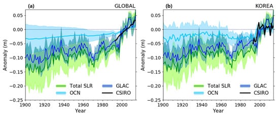
Figure 1.
Spatial mean time series of simulated ocean thermal expansion (light blue) and glacier (blue) contributions to SLR from ensemble means of CMIP6 models for (a) global and (b) Korean Peninsula with 95% confidence intervals (shaded). Green and black lines indicate total SLR from CMIP6 models and observation, respectively. The reference is the mean climatology of the PD (1995–2014) period.
In contrast, the observed SLR trend in the 2000–2014 period is nearly constant around the Korean Peninsula, whereas the simulated SLR (approximately 57 mm) tends to increase continuously (Figure 1b). The OCN and GLAC components contribute approximately 11 and 45 mm from 2000 to 2014, respectively. The OCN contribution around the Korean Peninsula is smaller than that of the global effect (approximately 21 mm) and the GLAC contribution is similar than that of the global effect (approximately 48 mm). This analysis indicates that the difference between simulated and observed SLR around the Korean Peninsula is due to the simulated uncertainty of the GLAC component.
3.2. Future Period
The first row in Figure 2a–c shows the 20 year averaged simulated future GMSL change for three climate targets (T15, T20, and T30) compared to the PD climatology from 1995 to 2014. The results of future projection indicate that SLR increased in most regions, and the regional patterns are similar to those reported previously [3,33,53]. Notable large changes occur in the Arctic, North Atlantic (northeastern coastal region of America), and Antarctic Circumpolar Current region (around 60° S). A comparison of each climate target show that the trends were more intense for T30 (Figure 2c). Additionally, the future projections for each climate target do not differ significantly between the four SSP-based scenarios (not shown) (Table 2). This suggests that the emission scenario has a small impact on the regional distribution of SLR in our results, and the distribution is similar to that of the recent CMIP6 study [26].
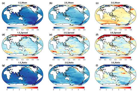
Figure 2.
Projection of total SLR from CMIP6 models (a–c) and their spread (d–f) for three Paris Climate targets (T15 (left column), T20 (mid column), and T30 (right column)). The ratio of mean and spread (g–i) of CMIP6 models is shown in the bottom row. The unit of SLR is m.
Table 2.
EoC values from CMIP6 ensemble based on each SSP scenario.
The spread of CMIP6 models (Figure 2d–f) was quantified as the minimum and maximum values, and occurs mainly in regions where the averaged SLR is large, in agreement with the results of previous studies [3,33,53]. The uncertainties associated with the ensemble do not vary significantly among the emission scenarios [7,26]. Thus, warming in the Arctic region, which is approximately two-fold higher than the global average [26,54], leads to a sea-ice melting process with large uncertainty. Additionally, the model response uncertainty increases for stronger responses, which is expected to result in high climate sensitivity [55]. Unlike the Arctic regions, the inter-model uncertainties of the North Atlantic and Antarctic Circumpolar Current region show a higher value at T30 compared to other warming levels (Figure 2f). Recent studies suggest that the large uncertainty in the North Atlantic is related to slower northward surface heat transport in CMIP6 models (affected by weakening Atlantic Meridional Overturning Circulation) [56,57,58,59]. In contrast, in the Antarctic Circumpolar Current region, a larger poleward shift of the westerly wind stress leads to the inter-model spread of CMIP6 models [59].
The lower panels in Figure 2 show the ratios of the mean and spread distributions, enabling assessment of the significance of the SLR trend. Although the ratio values are distributed in similar regions for three specific warming targets, higher values are projected in T30 (Figure 2i) relative to the other warming levels. A higher value for this ratio may be associated with smaller uncertainties. In most regions except the Arctic region, this ratio indicates a value of at least 1 above T15 (including T20 and T30). This means that intrinsic processes in the Arctic regions (e.g., sea-ice melting) of the coupled climate system also affect the high uncertainties in the Arctic region [60]. Overall, our results indicate that the SLR projection in T15 has a large uncertainty, whereas the SLR projections in T20 and T30 may be related to global warming above T15.
Figure 3 illustrates the spatial pattern of SLR projection around the Korean Peninsula. The distributions of SLR projection are similar for the three climate targets, although the SLR projections are more intense for T30 (approximately 20, 110, and 270 mm for T15, T20, and T30, respectively; Figure 3a–c). The ensemble spread of SLR projections is slightly larger in T30 than at the other two warming levels (Figure 3d–f). Thus, a higher ratio (Figure 3g–i) occurs in T30. In particular, the southern part of the East Sea shows a significantly high ratio, and this area is affected by the Kuroshio Warm Current [9,61]. As a result of continued global warming, warming currents will become stronger because of ocean warming in T30, affecting the trend in SLR [9,62,63,64].
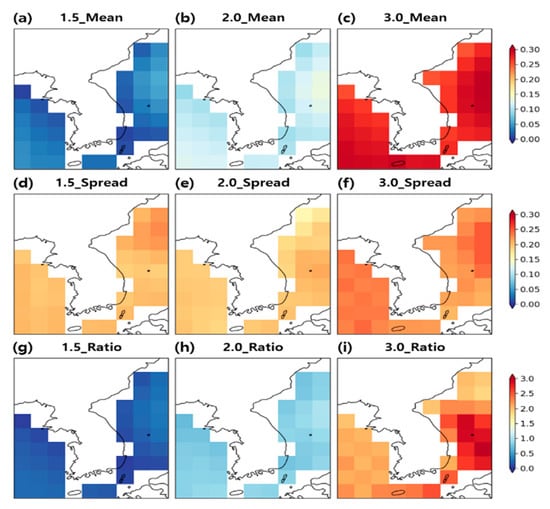
Figure 3.
Projection of total SLR around the Korean Peninsula from CMIP6 models (a–c) and their spread (d–f) for three Paris Climate targets (T15 (left column), T20 (mid column), and T30 (right column)). The ratio of mean and spread (g–i) of CMIP6 models is shown in the bottom row. The unit of SLR is m.
3.3. Drivers and Their Impacts
Figure 4a shows the GLAC contribution of future SLR projections for the three climate targets. In general, the median and spread of the CMIP6 ensemble show similar values in the global and KOR regions. Similar to the above results, the GLAC contribution trend increases as warming progresses (T15 < T20 < T30) and tends to accelerate. In addition, the spread of T30 skews significantly in the upward direction, whereas the spread of T15 and T20 have similar ranges and distributions in the upward and downward directions. This means that the calculated GLAC contributions and their related uncertainties are projected to increase as warming progresses. To determine the impact factors of this uncertainty, the future projections of the sea ice extent are illustrated in Figure 4b. The decreasing trend in the sea ice extent accelerates when warming in excess of 2.0 °C occurs in the Northern and Southern Hemispheres. This acceleration trend is very large in the Northern Hemisphere, with the upward spread of T20 much greater than that of T15. Thus, global warming above 1.5 °C may result in the crossing of a threshold for Arctic sea ice. Related evidence from previous studies suggests that summer sea ice in the Arctic will disappear after the first half of the 21st century because of rapid temperature increases [26,54].
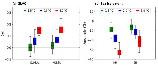
Figure 4.
(a) Projected changes in GLAC contributions (unit: m) for global and KOR regions and (b) projected changes in the sea ice extent (unit: %) for the Northern and Southern Hemispheres relative to during the pre-industrial period. Green, blue, and red boxes indicate the T15, T20, and T30 climate targets, respectively.
Table 2 shows the EoC of SLR and sea-ice melting. The trend accelerates after EoC because this step indicates when the climate variable is not consistent with the present-day (PD) trend. The EoC values of SLR on the global scale (2046–2063) and in KOR (2047–2058) are similar. Considering the median time of T15 and T20 from the CMIP6 models, the EoC of sea-ice melting in the Arctic (2031–2038) appears as global warming at near T15 or higher. In addition, the EoC of SLR (2046–2063) appears after that of sea ice in the Arctic, and the EoC of sea-ice melting in the Antarctic (2047–2067) occurs at a similar time to, or later than, that of SLR. Our results suggest that sea-ice melting due to global warming may lead to an increase in future SLR trends.
Figure 5 shows the OCN contribution of future SLR projections to the three climate targets. The increasing value between T20 and T30 is larger than that between T15 and T20. The median global (KOR region) value is 20 mm (10 mm), 40 mm (40 mm), and 90 mm (120 mm) for T15, T20, and T30, respectively. These values indicate that the OCN contribution to sea level change is more intense for KOR than for the global region with greater warming. In addition, the ensemble range (global/KOR) for T20 (90/120 mm) is significantly larger than that for T15 (80/100 mm), and the spread for T30 (290/290 mm) at the global scale shows a larger skew upwards, whereas the up and downward ranges are similar in KOR. Our results show that greater global warming leads to an increase in the OCN contribution and its upward uncertainty. As shown in Table 2, the EoC of “zostoga” (2036–2045) appears around the 2040s, which is similar to the time of the maximum of T15 warming and the median of T20 warming. Consequently, T15 warming may act as a trigger, and SLR may accelerate when the warming level is higher than that of T15.
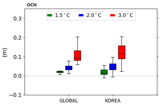
Figure 5.
Projected changes in OCN contributions (unit: m) for global and KOR regions relative to the pre-industrial period. Green, blue, and red boxes indicate the T15, T20, and T30 climate targets, respectively.
4. Discussion and Conclusions
To contribute to the IPCC AR6 WG1 (Working Group 1) report approved in August 2021, the global climate modeling research groups have reported several studies comparing the simulated results of CMIP5 and CMIP6 models. These studies report that CMIP6 models show better performance, even when considering their high climate sensitivity. It is essential to estimate future SLR projections from CMIP6 models because the IPCC AR method is the most authoritative calculation that considers anthropogenic forcing, and the high climate sensitivity of the CMIP6 model may influence the contribution of SLR (ocean thermal expansion and glacier melting). Additionally, previous studies have reported SLR projections for 2100, although future projections for related climate targets are needed to enable coastal decision making and adaptation planning. Therefore, we estimated future projections for SLR from CMIP6 models for three climate targets described by the Paris Agreement. Furthermore, we developed the EoC index and investigated its usefulness for SLR projections and evaluating related drivers.
Our findings demonstrate the relationship between SLR trends and warming levels based on new CMIP6 models. In a comparison of the results from each SSP scenario in AR6, the future projection at each climate target did not differ significantly between each of the four SSP-based scenarios. This result indicates that differences in the emission scenarios have a small impact on the SLR trend. Considering this, we intended to provide information from the CMIP6 ensemble on how the major drivers will affect SLR when climate targets are reached. Sea-ice melting and ocean thermal expansion are expected to increase with global warming, which will accelerate in response to T15 warming. Thus, T15 warming is a critical threshold (although not the exact tipping point). Beyond this critical point, the SLR will continue to rise for centuries to millennia because of continuing ocean warming and sea-ice melting, and will remain elevated for thousands of years because ocean variables react slowly (unlike atmospheric variables). Therefore, our findings provide information that is useful for ocean coastal policymakers. Additionally, an analysis method for calculating the SLR was created based on AR recommendations. This method can be applied in climate modeling to consider projection changes related to reference periods and enable easy comparison with the results of other studies. Overall, our results reveal future projections for the ocean ecosystem and can support the establishment of national climate change adaptation policies. Our results are summarized as follows:
- Throughout the analysis period, the GLAC component is responsible for most of the GMSL changes, rather than OCN. When all contributions are combined, the simulated global SLR (Korean Peninsula SLR) from 1900–1920 to 1995–2014 is 139 mm (128 mm), which is larger than that simulated using CMIP5 models (92/76 mm) [3].
- The global SLR projections are 60, 140, and 320 mm for T15, T20, and T30, respectively, relative to the PD period. The SLR projections in the marginal seas around the Korean Peninsula show similar trends (20, 110, and 270 mm for T15, T20, and T30, respectively) to those of the global values.
- The EoC values of SLR for global (2046–2063) and KOR (2047–2058) are similar. The EoC of SLR appears after the EoC of sea ice in the Arctic (2031–2038; near T15 time) and is similar to the EoC of sea-ice melting in the Antarctic (2047–2067). Overall, the trend in sea-ice melting may accelerate future SLR trends.
- The EoC of “zostoga” (related OCN contribution; 2036–2045) appears around the 2040s, which is similar to the time of the maximum of the T15 warming period and the median of the T20 warming period. Thus, T15 warming may act as a trigger, and SLR may accelerate when the warming level exceeds that of T15.
Author Contributions
Conceptualization, H.M.S. and S.S.; Data curation, J.K.; Formal analysis, H.M.S., J.K. and S.S.; Investigation, H.M.S. and J.-C.H.; Methodology, H.M.S. and Y.-H.B.; Resources, J.K.; Software, J.K.; Validation, J.K., H.M.S. and S.S.; Visualization, J.K. and H.M.S.; Writing—original draft, H.M.S.; Writing—review & editing, H.M.S., S.S., J.-C.H. and Y.-H.B.; Project administration, Y.-H.B. and Y.-H.K.; Funding acquisition, Y.-H.K. All authors have read and agreed to the published version of the manuscript.
Funding
This work was funded by the Korea Meteorological Administration Research and Development Program “Development and Assessment of IPCC AR6 Climate Change Scenarios” under Grant (KMA-2018-00321).
Institutional Review Board Statement
Not applicable.
Informed Consent Statement
Not applicable.
Data Availability Statement
The CMIP6 model results can be download from the ESGF node (https://esgf-node.llnl.gov/projects/cmip6).
Conflicts of Interest
The authors declare no conflict of interest.
References
- Gattuso, J.-P.; Hock, R. Special Report on the Ocean and Cryosphere in a Changing Climate; Portner, H.-O., Roberts, D.C., Masson-Delmotte, V., Zhai, P., Tignor, M., Poloczanska, E., Mintenbeck, K., Alegria, A., Nicolai, M., Lkem, A., et al., Eds.; IPCC: Geneva, Switzerland, 2019. [Google Scholar]
- Nicholls, R.J.; Cazenave, A. Sea-level rise and its impact on coastal zones. Science 2010, 328, 1517–1520. [Google Scholar] [CrossRef] [PubMed]
- Slangen, A.B.A.; Meyssignac, B.; Agosta, C.; Champollion, N.; Church, J.A.; Fettweis, X.; Ligtenberg, S.R.M.; Marzeion, B.; Melet, A.; Palmer, M.D.; et al. Evaluating model simulations of twentieth-century sea level rise. Part 1: Global mean sea level change. J. Clim. 2017, 30, 8539–8563. [Google Scholar] [CrossRef]
- Choi, J.Y.; Kim, J.H. Study on Necessity of Creating New Sea City; Korea Maritime Institute: Busan, Korea, 2019. [Google Scholar]
- Clark, P.U.; Church, J.A.; Gregory, J.M.; Payne, A.J. Recent progress in understanding and projecting regional and global mean sea level change. Curr. Clim. Chang. Rep. 2015, 1, 224–246. [Google Scholar] [CrossRef]
- Abadie, L.M.; Jackson, L.P.; sainz de Murieta, E.; Jevrejeva, S.; Galarraga, I. Comparing urban coastal flood risk in 136 cities under two alternative sea-level projections: RCP 8.5 and an expert opinion-based high end scenario. Ocean. Coast. Manag. 2020, 193, 105249. [Google Scholar] [CrossRef]
- IPCC. Summary for Policymakers. In Climate Change 2013: The Physical Science Basis; Contribution of working group I to the fifth assessment report of IPCC the intergovernmental panel on climate change; Stocker, T.F., Qin, D., Plattner, G.-K., Tignor, M.M.B., Allen, S.K., Boschung, J., Nauels, A., Xia, Y., Bex, V., Midgley, P.M., Eds.; Cambridge University Press: Cambridge, UK, 2014; pp. 3–29. [Google Scholar]
- Heo, T.-K.; Kim, Y.; Boo, K.-O.; Byun, Y.-H.; Cho, C. Future sea-level projections over the seas around Korea from CMIP6 simulations. Atmosphere 2018, 28, 25–35. [Google Scholar]
- Sung, H.M.; Kim, J.; Lee, J.-H.; Shim, S.; Boo, K.-O.; Ha, J.-C.; Kim, Y.-H. Future Changes in the Global and Regional Sea Level Rise and Sea Surface Temperature Based on CMIP6 Models. Atmosphere 2021, 12, 90. [Google Scholar] [CrossRef]
- UNFCCC. The Paris Agreement. United Nations Framework Convention on Climate Change, 2015. Available online: http://unfccc.int/paris_agreement/items/9485.php (accessed on 26 October 2017).
- Mengel, M.; Nauels, A.; Rogelj, J.; Schleussner, C.-F. Committed sea level rise under the Paris Agreement and the legacy of delayed mitigation action. Nat. Commun. 2008, 9, 1–10. [Google Scholar] [CrossRef]
- Wigley, T.M.L. The Paris warming targets: Emissions requirements and sea level consequences. Clim. Chang. 2018, 147, 31–45. [Google Scholar] [CrossRef]
- IPCC. Summary for Policymakers. In Global Warming of 1.5 °C. An IPCC Special Report on the Impacts of Global Warming of 1.5 °C Above Pre-Industrial Levels and Related Global Greenhouse Gas Emission Pathways, in the Context of Strengthening The Global Response to the Threat of Climate Change, Sustainable Development, and Efforts to Eradicate Poverty; Masson-Delmotte, V., Zhai, P., Portner, H.O., Roberts, D., Skea, J., Shukla, P.R., Pirani, A., Moufouma-Okia, W., Pean, C., Pidcock, R., et al., Eds.; IPCC: Geneva, Switzerland; Available online: https://www.ipcc.ch/sr15/download/ (accessed on 25 September 2021).
- Jevrejeva, S.; Jackson, L.P.; Grinsted, A.; Lincke, D.; Marzeion, B. Flood damage costs under the sea level rise with warming of 1.5 °C and 2 °C. Environ. Res. Lett. 2018, 13, 074014. [Google Scholar] [CrossRef]
- Qu, Y.; Kiu, Y.G.; Jevrejeva, S.; Jackson, L.P. Future Sea level rise along the coast of China and adjacent region under 1.5 °C and 2.0 °C global warming. Adv. Clim. Chang. Res. 2020, 11, 227–238. [Google Scholar] [CrossRef]
- O’Neill, B.C.; Tebaldi, C.; van Vuuren, D.P.; Eyring, V.; Friedlingstein, P.; Hurtt, G.; Knutti, R.; Kriegler, E.; Lamarque, J.-F.; Lwe, J.; et al. The Scenario Model Intercomparison Project (ScenarioIP) for CMIP6. Geosci. Model. Dev. 2016, 9, 3461–3482. [Google Scholar] [CrossRef]
- Knutti, R.; Furrer, R.; Tebaldi, C.; Cermak, J.; Meehl, G.A. Challenges in combining projections from multiple climate models. J. Clim. 2010, 23, 2739–2758. [Google Scholar] [CrossRef]
- Williams, D.; Balaji, B.; Cinquini, L.; Denvil, S.; Duffy, D.; Evans, B.; Ferraro, R.; Hansen, R.; Lautenschlager, M.; Trenham, C. A global repository for planet-sized experiments and observations. Bull. Am. Meteorol. Soc. 2016, 97, 803–816. [Google Scholar] [CrossRef]
- Tamisiea, M.E.; Mitrovia, J.X. The moving boundaries of sea level change: Understanding the origins of geographic variability. Oceanography 2011, 24, 24–39. [Google Scholar] [CrossRef]
- Wada, Y.; Bierkens, M.F.P.; de Roo, A.; Dirmeyer, P.A.; Famiglietti, J.S.; Hanasaki, N.; Konar, M.; Liu, J.; Schmied, H.M.; Oki, T.; et al. Human-water interface in hydrological modeling: Current status and future directions. Hydrol. Earth Syst. Sci. 2017, 21, 4169–4193. [Google Scholar] [CrossRef]
- Rayner, N.A.; Parker, D.E.; Horton, E.B.; Folland, C.K.; Alexander, V.; Rowell, D.P.; Kent, E.C.; Kaplan, A. Global analyses of sea surface temperature, sea ice, and night marine air temperature since the late nineteenth century. J. Geophys. Res. 2003, 108, 4407. [Google Scholar] [CrossRef]
- Church, J.A.; White, N.J. Sea-level rise from the late 19th to the early 21st century. Surv. Geophys. 2011, 32, 585–602. [Google Scholar] [CrossRef]
- Mora, C.; Frazier, A.; Longman, R.; Dacks, R.S.; Walton, M.M.; Tong, E.J.; Sanchez, J.J.; Kaiser, L.R.; Stender, Y.O.; Anderson, J.M.; et al. The projected timing of climate departure from recent variability. Nature 2013, 502, 183–187. [Google Scholar] [CrossRef] [PubMed]
- Maraun, D. When will trends in European mean and heavy daily precipitation emerge? Environ. Res. Lett. 2013, 8, 014004. [Google Scholar] [CrossRef]
- Hawkins, E.; Sutton, R. Time of emergence of climate signals. Geophys. Res. Lett. 2012, 39, l01702. [Google Scholar] [CrossRef]
- Tebaldi, C.; Debeire, K.; Eyring, V.; Fischer, E.; Fyfe, J.; Friedlingstein, P.; Knutti, R.; Lowe, J.; O’Neill, B.; Sanderson, B.; et al. Climate model projections from the Scenario Model Intercomparison Project (ScenarioMIP) of CMIP6. Earth Syst. Dynam. 2021, 12, 253–293. [Google Scholar] [CrossRef]
- Boo, K.-O.; Shim, S.; Kim, J.-E.; Byun, Y.-H.; Cho, C.H. Emergence of Anthropogenic Warming over South Korea in CMIP5 Projections. J. Clim. Chang. Res. 2016, 7, 421–426. [Google Scholar] [CrossRef]
- Palmer, M.D.; Gregory, J.M.; Bagge, M.; Calvert, D.; Hagedoorn, J.M.; Howard, T.; Klemann, V.; Lowe, J.A.; Roberts, C.D.; Slangen, A.B.A.; et al. Exploring the drivers of global and local sea level change over the 21st century and beyond. Earth’s Future 2020, 8, e2019EF001413. [Google Scholar] [CrossRef]
- Marzeion, B.; Champollion, N.; Haeberli, W.; Langley, K.; Leclercq, P.; Paul, F. Observation based estimates of global glacier mass change and its contribution to sea-level change. In Integrative Study of the Mean Sea Level and Its Components; Cazenave, A., Champollion, N., Paul, F., Benveniste, J., Eds.; Spinger: Cham, Switzerland, 2017; pp. 107–132. [Google Scholar]
- Radic, V.; Hock, R. Regional and global volumes of glaciers derived from statistical upscaling of glacier inventory data. J. Geophys. Res. 2010, 115, F01010. [Google Scholar] [CrossRef]
- Frezzotti, M.; Scarchilli, C.; Becagli, S.; Proposito, M.; Urbini, S. Synthesis of the Antarctic surface mass balance during the last 800 yr. Cryosphere 2013, 7, 303–319. [Google Scholar] [CrossRef]
- Slangen, A.B.A.; van de Wal, R.S.W. An assessment of uncertainties in using volume area modeling for computing the twenty first century glacier contribution to sea level change. Cryosphere 2011, 5, 673–686. [Google Scholar] [CrossRef]
- Slangen, A.B.A.; Carson, M.; Katsman, C.A.; van de Wal, R.S.W.; Köhl, A.; Vermeersen, L.L.A.; Stammer, D. Projecting twenty-first-century regional sea-level changes. Clim. Chang. 2014, 124, 317–332. [Google Scholar] [CrossRef]
- Fettweis, X.; Box, J.E.; Agosta, C.; Amory, C.; Kittel, C.; Lang, C.; Van As, D.; Machguth, H.; Gallée, H. Reconstructions of the 1900-2015 Greenland ice sheet surface mass balance using the regional climate MAR model. Cryosphere 2017, 11, 1015–1033. [Google Scholar] [CrossRef]
- Cook, A.J.; Vaughan, D.G. Overview of area changes of the ice shelves on the Antarctic Peninsula over the past 50 years. Cryosphere 2010, 4, 77–98. [Google Scholar] [CrossRef]
- Pritchard, H.D.; Ligtenberg, S.R.M.; Fricker, H.A.; Vaughan, D.G.; Broeke, M.R.V.D.; Padman, L. Antarctic ice sheet loss driven by basal melting of ice shelves. Nature 2012, 484, 502–505. [Google Scholar] [CrossRef]
- Nick, F.M.; Vieli, A.; Andersen, M.L.; Joughin, I.R.; Payne, A.; Edwards, T.L.; Pattyn, F.; Van De Wal, R.S.W. Future sea-level rise from Greenland’s main outlet glaciers in a warming climate. Nature 2010, 497, 235–238. [Google Scholar] [CrossRef]
- Goelzer, H.; Huybrechts, P.; Furst, J.J.; Nick, F.; Andersen, M.; Edwards, T.; Fettweis, X.; Payne, A.; Shannon, S. Sensitivity of Greenland ice sheet projections to model formulations. J. Glaciol. 2013, 59, 733–749. [Google Scholar] [CrossRef]
- Peltier, W.R. Global glacial isostasy and the surface of the ice-age earth: The ICE-5G(VM2) model and GRACE. Annu. Rev. Earth Planet. Sci. 2004, 32, 111–149. [Google Scholar] [CrossRef]
- Slangen, A.B.A.; Katsman, C.A.; van de Wal, R.S.W.; Vermeersen, L.L.A.; Riva, R.E.M. Towards regional projections of twenty-first century sea level change based on IPCC SRES scenarios. Clim. Dyn. 2012, 38, 1191–1209. [Google Scholar] [CrossRef]
- Meehl, G.A.; Stocker, T.F.; Collins, W.D.; Friedlingstein, P.; Gaye, A.; Gregory, J.; Kitoh, A.; Knutti, R.; Murphy, J.; Noda, A.; et al. Climate Change 2007: The Physical Science Basis. Contribution of Working Group 1 to the 4th Assessment Report of the Intergovernmental Panel on Climate Change; Cambridge University Press: Cambridge, UK, 2007. [Google Scholar]
- Frederikse, T.; Riva, R.E.M.; King, M.A. Ocean bottom deformation due to present-day mass redistribution and its impact on sea-level observations. Geophys. Res. Lett. 2017, 44, 12–306. [Google Scholar] [CrossRef]
- Martinec, Z.; Klemann, V.; Vander Wal, W.; Riva, R.E.; Spada, G.; Sun, Y.; Melini, D.; Kachuck, S.; Barletta, V.; Simon, K.; et al. A benchmark study of numerical implementations of the sea level equation in GIA modeling. Geophys. Res. Lett. 2018, 215, 389–414. [Google Scholar]
- Gleckler, P.J.; Durack, P.J.; Stouffer, R.J.; Johnson, G.C.; Forest, C.E. Industrial-era global ocean heat uptake doubles in recent decades. Nat. Clim. Chang. 2016, 6, 394–398. [Google Scholar] [CrossRef]
- Glecker, P.J.; AchutaRao, K.; Gregory, J.M.; Santer, B.D.; Taylo, K.E.; Wigley, T.M.L. Krakatoa lives: The effect of volcanic eruptions on ocean heat content and thermal expansion. Geophys. Res. Lett. 2006, 33, L17702. [Google Scholar] [CrossRef]
- von Schuckmann, K.; Palmer, M.D.; Trenberth, K.E.; Cazenave, A.; Chambers, D.; Champollion, N.; Hansen, J.; Josey, S.A.; Loeb, N.; Mathieu, P.P.; et al. An imperative to monitor Earth’s energy imbalance. Nat. Clim. Chang. 2016, 6, 138–144. [Google Scholar] [CrossRef]
- Bjørk, A.A.; Kjær, K.H.; Korsgaard, N.J.; Khan, S.A.; Kjeldsen, K.K.; Andresen, C.S.; Box, J.E.; Larsen, N.K.; Funder, S. An aerial view of 80 years of climate related glacier fluctuations in southeast Greenland. Nat. Geosci. 2012, 5, 138–144. [Google Scholar] [CrossRef]
- Marzeion, B.; Cogley, J.G.; Richter, K.; Parkes, D. Attribution of global glacier mass loss to anthropogenic and natural causes. Science 2014, 345, 919–921. [Google Scholar] [CrossRef] [PubMed]
- Marcos, M.; Amores, A. Quantifying anthropogenic and natural contributions to thermosteric sea level rise. Geophys. Res. Lett. 2014, 41, 2502–2507. [Google Scholar] [CrossRef]
- Zelinka, M.D.; Myers, T.A.; McCoy, D.T.; Po-Chedley, S.; Caldwell, P.M.; Ceppi, P.; Klein, S.A.; Taylor, K.E. Causes of higher climate sensitivity in CMIP6 models. Geophys. Res. Lett. 2020, 47, e2019GL085782. [Google Scholar] [CrossRef]
- Sun, M.-A.; Sung, H.M.; Kim, J.; Boo, K.-O.; Lim, Y.-J.; Marzin, C.; Byun, Y.-H. Climate sensitivity and feedback of a new coupled model(K-ACE) to idealized CO2 forcing. Atmosphere 2020, 11, 1218. [Google Scholar] [CrossRef]
- Chambers, D.P.; Cazenave, A.; Champollion, N.; Dieng, H.; Llovel, W.; Forsberg, R.; von Schuckmann, K.; Wada, Y. Evaluation of the global mean sea level budget between 1993 and 2014. Surv. Geophys. 2017, 38, 309–327. [Google Scholar] [CrossRef]
- Ferrero, B.; Tonelli, M.; Marcello, F.; Wainer, I. Long-term regional dynamical sea level changes from CMIP6 projections. Adv. Atmos. Sci. 2021, 38, 157–167. [Google Scholar] [CrossRef]
- Sung, H.M.; Kim, J.; Shim, S.; Seo, J.; Kwon, S.-H.; Sun, M.-A.; Moon, H.; Lee, J.-H.; Lim, Y.-J.; Boo, K.-O.; et al. Climate change projection in the twenty-first century simulated by NIMS-KMA CMIP6 model based on new GHGs concentration pathways. Asia-Pac. J. Atmos. Sci. 2021, 34, 1–12. [Google Scholar] [CrossRef]
- Lehner, E.; Deser, C.; Maher, N.; Marotzke, J.; Fischer, E.M.; Brunner, L.; Knutti, R.; Hawkins, E. Partitioning climate projection uncertainty with multiple large ensembles and CMIP5/6. Earth Syst. Dyn. 2020, 11, 491–508. [Google Scholar] [CrossRef]
- Bilbao, R.A.F.; Gregory, J.M.; Bouttes, N. Analysis of the regional pattern of sea level change due to ocean dynamics and density change for 1993-2099 in observations and CMIP5 AOGCMs. Clim. Dyn. 2015, 45, 2647–2666. [Google Scholar] [CrossRef]
- Caesar, L.; Rahmstorf, S.; Robinson, A.; Feulner, G.; Saba, V. Observed fingerprint of a weakening Atlantic Ocean overturning circulation. Nature 2018, 556, 191–196. [Google Scholar] [CrossRef] [PubMed]
- Keil, P.; Mauritsen, T.; Jungclaus, J.; Hedemann, C.; Olonscheck, D.; Gosh, R. Multiple drivers of the North Atlantic warming hole. Nat. Clim. Chang. 2020, 10, 667–671. [Google Scholar] [CrossRef]
- Lyu, K.; Zhang, X.B.; Church, J.A. Regional dynamic sea level simulated in the CMIP5 and CMIP6 models: Mean biases, future projections, and their linkages. J. Clim. 2020, 33, 6377–6398. [Google Scholar] [CrossRef]
- Deser, C.; Lehner, F.; Rodgers, K.B.; Ault, T.; Delworth, T.L.; DiNezio, P.N.; Fiore, A.; Frankignoul, C.; Fyfe, J.C.; Horton, D.E.; et al. Insights from Earth system model initial condition large ensembles and future prospects. Nat. Clim. Chang. 2020, 10, 277–286. [Google Scholar] [CrossRef]
- Yoon, J.J.; Kim, S.I. Analysis of long period sea level variation on tidal station around the Korea Peninsula. J. Korean Soc. Hazard. Mitig. 2012, 12, 299–305. [Google Scholar] [CrossRef][Green Version]
- Wu, L.; Cai, W.; Zhang, L.; Nakamura, H.; Timmermann, A.; Joyce, T.; McPhaden, M.J.; Alexander, M.; Qiu, B.; Visbeck, M.; et al. Enhanced warming over the global subtropical western boundary currents. Nat. Clim. Chang. 2012, 2, 161–166. [Google Scholar] [CrossRef]
- Yeh, S.-W.; Kim, C.-H. Recent warming in the Yellow/East China Sea during winter and the associated atmospheric circulation. Cont. Shelf Res. 2010, 30, 1428–1434. [Google Scholar] [CrossRef]
- Gordon, A.L.; Giulivi, C.F. Pacific decadal oscillation and sea level in the Japan/East Sea. Deep Sea Res. Part I Oceanogr. Res. Pap. 2004, 51, 653–663. [Google Scholar] [CrossRef]


Publisher’s Note: MDPI stays neutral with regard to jurisdictional claims in published maps and institutional affiliations. |
© 2021 by the authors. Licensee MDPI, Basel, Switzerland. This article is an open access article distributed under the terms and conditions of the Creative Commons Attribution (CC BY) license (https://creativecommons.org/licenses/by/4.0/).