Interannual to Interdecadal Variability of the Southern Yellow Sea Cold Water Mass and Establishment of “Forcing Mechanism Bridge”

Abstract

The Yellow Sea cold water mass (YSCWM) occupies a wide region below the Yellow Sea (YS) thermocline in summer which is the most conservative water and may contain clearer climate signals than any other water masses in the YS. This study investigated the low-frequency variability of the southern YSCWM (SYSCWM) and established the “forcing mechanism bridge” using correlation analysis and singular value decomposition. On the interannual timescale, the southern oscillation can affect the SYSCWM through both the local winter monsoon (WM) and the sea surface net heat flux. On the decadal timescale, the Pacific decadal oscillation (PDO) can affect the SYSCWM via two “bridges”. First, the PDO affects the SYSCWM intensity by Aleutian low (AL), WM, and surface air temperature (SAT). Second, the PDO affects the SYSCWM by AL, WM, Kuroshio heat transport, and Yellow Sea warm current. The Arctic oscillation (AO) affects the SYSCWM by the Mongolian high, WM, and SAT. Before and after the 1980s, the consistent phase change of the PDO and the AO contributed to the significant decadal variability of the SYSCWM. Finally, one simple formula for predicting the decadal variability of SYSCWM intensity was established using key influencing factors.

1. Introduction

The Yellow Sea (YS) is a shallow and semienclosed marginal sea of the Pacific Ocean, bordered by the Chinese mainland to the west, the Korean peninsula to the east, and the Bohai Bay to the north. There is a remnant of cold water (<10 °C) under the seasonal thermocline in the central trough of the YS which is referred as the Yellow Sea cold water mass (YSCWM) [1]. The YSCWM occupies almost 30% of the YS area and is present throughout the whole summer every year which becomes one of the most important characteristics of the YS. The YSCWM has a large impact on the hydrographic features and the phytoplankton biomass and production in the YS [2,3,4]. There are strong temperature gradients between cold water masses and surrounding waters, which generate special hydrodynamic processes, e.g., the bottom thermal front, cyclonic gyre above the cold water mass [5,6]. The YSCWM is regarded as a nutrient-rich pool that contributes to the subsurface chlorophyll maximum phenomenon during summer and therefore affects primary production [7,8,9,10,11]. The key species of zooplankton (Calanus sinicus) is favored to survive the hot summer in the YSCWM [12]. Consequently, the demersal fish stocks are closely related to the YSCWM intensity [13,14]. The diverse characteristics of the YSCWM have drawn the attention of many international scholars.

He et al. [1] first studied the formation and properties of the YSCWM and identified that the water mass was locally formed during the previous winter by sea surface cooling and strong vertical mixing. After this pioneering work, there were many studies on the seasonal evolution of the YSCWM and its formation mechanism [15,16,17,18,19,20,21]. The formation mechanism of the YSCWM including the strong tidal mixing, wind stirring, warming surface, winter air temperature, thermocline, warm current and topography [22,23].

Many researchers also have explored interannual and long-term variability of the YSCWM. Hu and Wang [18] adopted the empirical orthogonal function (EOF) method to find that the vertical circulation in the southern YS is correlated with the surface wind curl on the interannual timescale. Park et al. [21] found there are three cold events and two warm events in the west of southern YSCWM (SYSCWM) using the EOF method and the variation of the YSCWM is influenced by sea level pressure (SLP), surface air temperature (SAT), sea surface temperature (SST), Pacific decadal oscillation (PDO), and Arctic oscillation (AO). Jiang et al. [24] found the Kuroshio meander always induces a warmer YSCWM in the following year and the temperature of the northern YSCWM has a linear trend which is related to the winter air temperature. Wei et al. [25] found the interannual variation of winter water temperature in the YS is driven by the lateral heat input from the intrusive Yellow Sea warm current (YSWC). Yang et al. [26] studied the interannual variation of the southern limit of the YSCWM and found that the colder SST in winter is associated with the increased southern limit in the following summer. Li et al. [27] found winter AO and PDO modulate the decadal variability of the YSCWM by the local heat flux and wind stress, and in summer, El Niño/southern oscillation (ENSO) is the dominant factor influencing the YSCWM. Zhu et al. [28] showed that the air–sea heat flux is the dominant factor influencing the YSCWM’s intensity.

Previous studies of the variability of the SYSCWM (e.g., Park et al. [21]; Li et al. [27]) have identified that remote factors affect local factors but the forcing mechanisms have not been discussed. Therefore, the objectives of this study were to characterize the interannual and decadal variability of the SYSCWM and to establish the “forcing mechanism bridge” from remote factor to SYSCWM. Remote forcing factors do not usually act directly on local factors. Instead, intermediate factors generally act as a “bridge” connecting the remote and local factors. This study established several “bridges” via which remote factors (e.g., ENSO, PDO, and AO) might influence local factors (e.g., the winter monsoon (WM), sea surface net heat flux (NHF), SAT, and YSWC) through intermediate factors (e.g., Kuroshio heat transport (KHT), Mongolian high (MH), and Aleutian low (AL)) and ultimately affect the SYSCWM on interannual and decadal timescales. This is helpful for further understanding the forcing mechanisms of climate factors. One simple formula for predicting the decadal variability of SYSCWM intensity was established using key influencing factors.

2. Materials and Methods

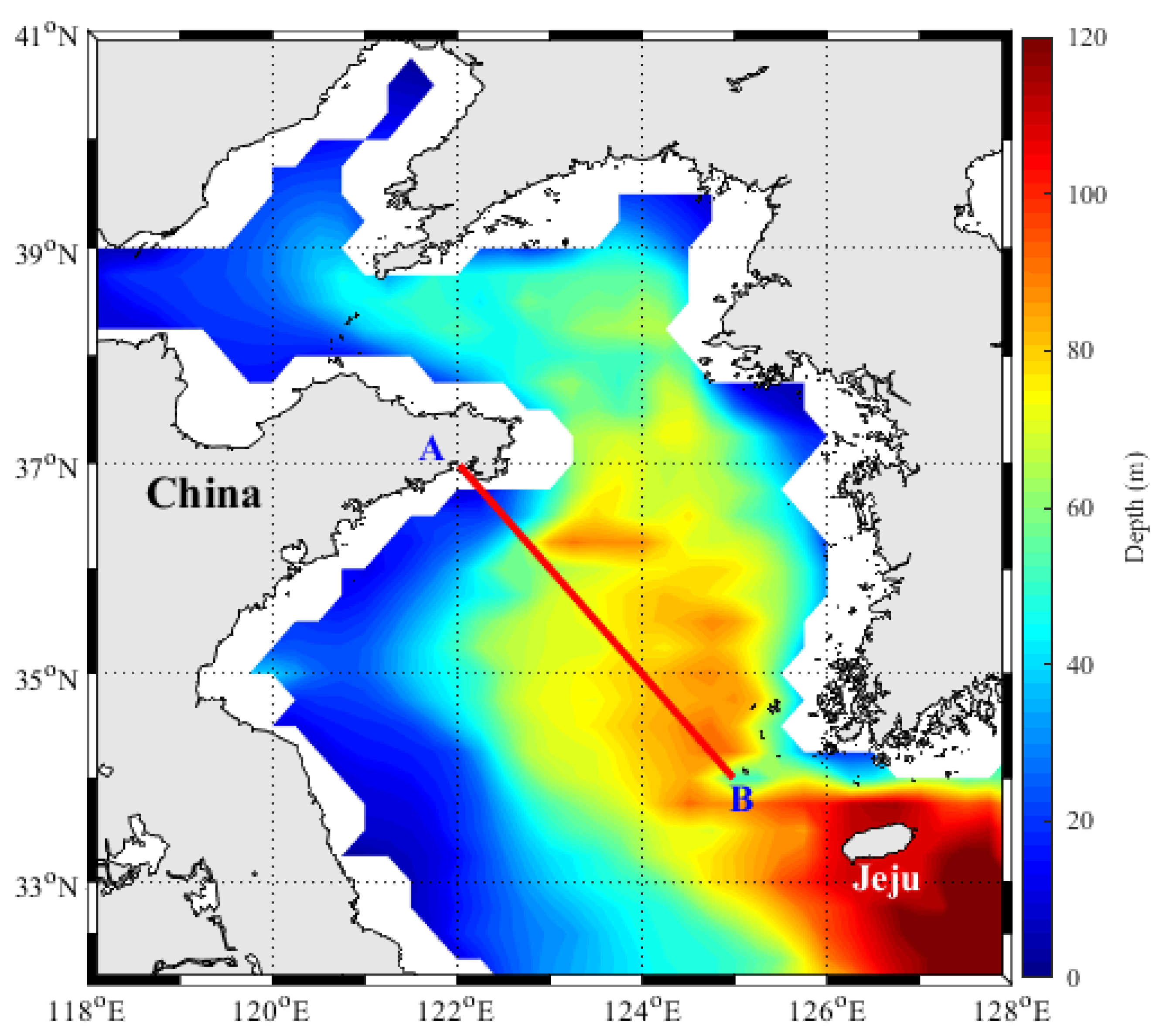
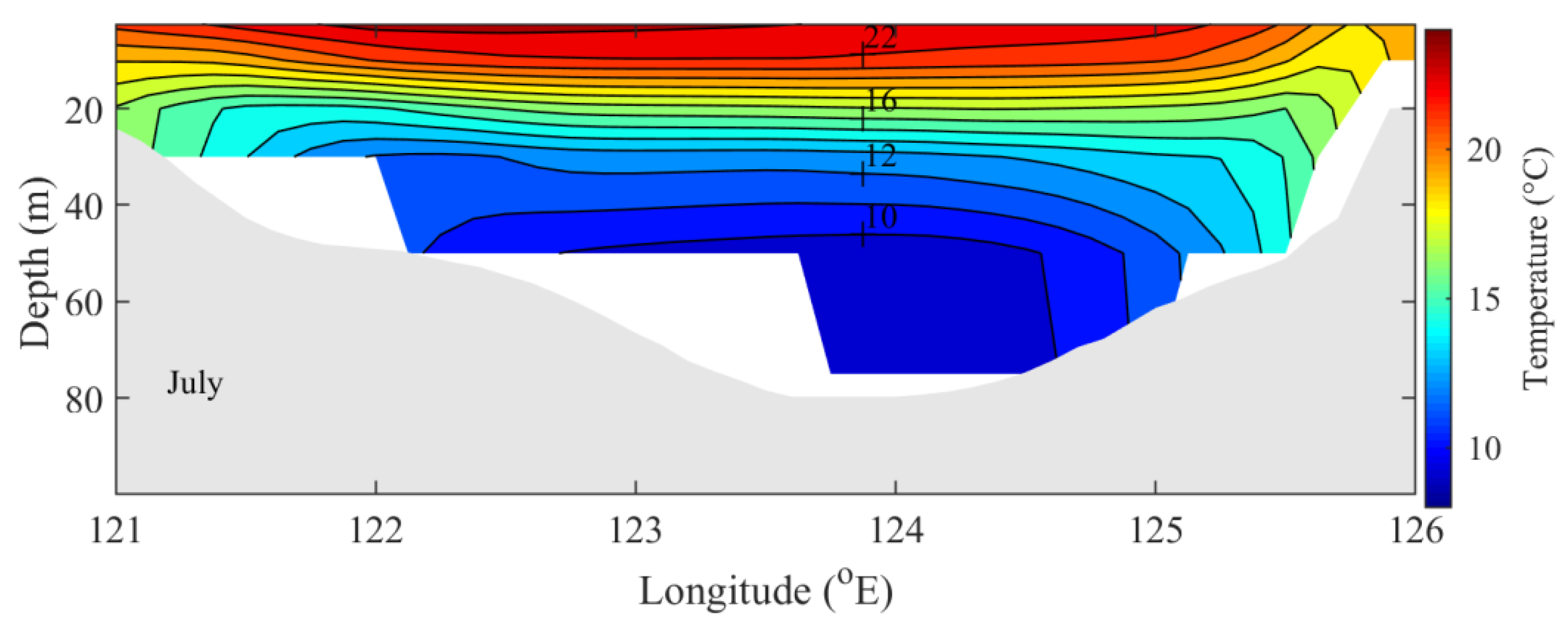
2.1. Study Area

The depth of the thermocline in YS is about 20 m. In summer, there is cold front doming up to the surface and separating the upper layer into two warm water lenses [18]. The YSCWM is traditionally defined as the cold water lower than 10 °C under the seasonal thermocline in the central trough of the YS in summer [1]. The stirring of strong northerly wind during winter results in vertically well-mixed waters from the surface to the bottom. In summer, increased solar radiation drives strong stratification which prevents water from vertical mixing. Cold water that forms in winter maintains its temperature beneath the stratified thermocline which forms the YSCWM. The topography of the YS from the ETOPO1 dataset (https://www.ngdc.noaa.gov/mgg/global/, accessed on 17 November 2021) is shown in Figure 1.

2.2. CORA Data

Ocean reanalysis datasets, which have better spatiotemporal coverage than observational records, are suitable for supporting investigation of the features of the entire YSCWM and its response to climate variability. Therefore, the China Coastal Waters and Adjacent Seas Reanalysis (CORA) data were used in this study.

The CORA data are based on an oceanic dynamical model, which incorporates wave breaking parameterization and tidal mixing processes, together with assimilation of in situ observed temperature and salinity profiles. CORA data have been validated using independent observations in previous studies, and the results have shown that CORA data are well suited for the simulation of both the temperature–salinity structure and the mesoscale and large-scale circulations of the western North Pacific Ocean including the YS [29]. The CORA dataset covers a 54-year period from January 1958 to December 2011. The domain of 10° S–52° N, 99°–150° E includes the Bohai Sea, YS, East China Sea, South China Sea, and adjacent seas. The dataset consists of monthly mean fields with horizontal resolution of 0.125°and 35 vertical levels with determined depth, e.g., 2.5 m, 10 m, 20 m, 30 m. Figure 2 presents the climatological temperature in the YS in July along 35° N from CORA data. It can be seen that the CORA data can well represent the mixing layer, tidal fronts, and the bottom cold water within the YS.

2.3. Climate and Intensity Indices

According to previous studies [21,27,30], remote factors (ENSO, PDO, AO), local factors (WM, NHF, SAT, YSWC), and intermediate factors (KHT, MH, AL) can all affect the interannual or decadal variability of the SYSCWM. The Nino3.4 index is one of several ENSO indicators downloaded from https://psl.noaa.gov/gcos_wgsp/Timeseries/Nino34/, accessed on 17 November 2021. Its positive values represent El Niño events and the negative values represent La Niña events. The PDO index (http://research.jisao.washington.Edu/pdo, accessed on 17 November 2021) is defined as the leading principal component of monthly SST north of 20° N in the North Pacific. The AO index (http://www.cpc.ncep.noaa.gov/products/precip/CWlink, accessed on 17 November 2021) is the dominant pattern of nonseasonal SLP variability north of 20° N. The local WM index is defined as the anomaly of winter meridional wind speed averaged over the domain 32.5–37.5° N, 120–127.5° E. The NHF and SAT indices are defined as the anomaly of winter sea surface net heat flux and the anomaly of winter surface air temperature, respectively, averaged over the same domain. Based on the CORA data, we defined the YSWC intensity index as the distance of the northern limit of the 10 °C isotherm from the reference latitude of 33° N in January; the greater the distance, the more intense the intrusion of the YSWC. KHT is calculated based on the temperature data along the PN section referring to Zhang et al. [31]. MH index is defined as the surface integral of the potential height difference over a specific area in winter referring to Sun et al. [32]. AL index is defined similarly to MH referring to Wang et al. [33]. The wind field, heat flux, and pressure data used in the definitions of the WM, NHF, SAT, MH, and AL were obtained from the National Centers for Environmental Prediction/National Center for Atmospheric Research reanalysis (NCEP) [34].

With reference to previous research [26,27], we also defined an index of SYSCWM intensity, i.e., the anomalies of averaged temperature (T-10) of the SYSCWM, which is defined as the cold water lower than 10 °C in the bottom of the south YS, in July, as shown in Figure 3. Based on the Mann–Kendall test, the T-10 index has a significant increasing trend of 0.0022 °C/year during 1958–2011, associated with recent global warming [35,36,37].

2.4. Methods

The time series data used in this study included both interannual and decadal variability. The interannual variability was obtained by removing the climatological monthly means. The decadal variability was obtained by applying 7-year low-pass filtering to remove the most significant interannual signal, i.e., ENSO. Some summer (averaged from June to August) and winter (averaged from December to February) climate indices were used to examine the effects of different seasonal climate forcings. For instance, 1958 winter (summer) is an average of December 1957, January 1958, and February 1958 (June, July, and August 1958).

EOF method is used to analyze the spatial-temporal variation of the YSCWM. It can reflect the main information of meteorological field in a few modes. To extract the dominant mode of temperature in the southern YS, the EOF method was used on the interannual time series.

Strong correlation with a certain climate index would imply that the corresponding climate factor is associated with YSCWM variability; therefore, examination of the correlation could represent a quick guide to the relationships of the background variables. In addition, correlation with a lag/lead time would reveal whether the two time series are related remotely and which of the time series leads. This is achieved by cross-correlation function in present study. A positive lag indicates that the climate index leads the SYSCWM. The correlation coefficients reported in this paper are all statistically significant at the 90% confidence level.

In addition to correlation analysis, we also used singular value decomposition (SVD) analysis to identify the covariance between two variables. The purpose of SVD is to separate regions of high correlation between paired fields, to elucidate the spatial structure of the correlation field between the paired fields and to determine their respective contributions to the correlation field. The results of the SVD analysis include a spatial pattern, normalized time series, and heterogeneous correlation pattern. We only present results of the first SVD mode because the first mode accounts for the largest fraction of variance. As can be seen from Figure 4 below, the YSCWM can be clearly seen in temperature field at 50 m depth and in July, the surface covered by the 10 °C isotherm is the largest. Therefore, in SVD analysis, the July temperature anomaly at the depth of 50 m in the southern YS was used to represent SYSCWM variability. In fact, the temperature field of YSCWM at the 50 m depth has been frequently used in other studies [20,21,28,38,39,40]. In this paper, we conducted SVD analysis on climate index and SYSCWM index at the lead time determined in the correlation analysis.

Generally, the effect of remote factors is manifest through local or intermediate forcing. Therefore, we first examined how local or intermediate forcings might affect the SYSCWM. Then, we examined how the remote forcings might affect the local or intermediate factors. Finally, we explored the direct links between the remote factors and the SYSCWM, and we established several “forcing mechanism bridges” through which the remote factors might affect the local or intermediate factors that in turn affect the variability of SYSCWM intensity.

3. Results

Figure 4 illustrates the distribution of the climatological monthly averaged temperature (°C) during 1958–2011 at the depth of 50 m in the YS based on the CORA data. It can be seen that the bottom water temperature in the YS warms gradually from winter to spring and that the SYSCWM (bottom water colder than 10 °C), which disappears in autumn, can be identified clearly in summer. Further, the lower part of all rectangles in Figure 4 contains warmer water throughout the year which is the YSWC in autumn, winter, and spring or the surrounding warmer water in summer [19,41,42].

3.1. Interannual Variability of the SYSCWM

The EOF method was used on the interannual components of temperature along section A–B (Figure 1), which spans the whole area of the southern YS, to investigate the interannual spatiotemporal characteristics of the SYSCWM. In the EOF analysis, the interannual variation signal of surface water is much stronger than that of the SYSCWM. Therefore, we extracted the data deeper than 40 m along section A–B for EOF analysis. The first EOF mode that represents the surface temperature variability of the southern YS explained 45% of the total variance but were not of concern in this study. Therefore, they are not presented. The second EOF mode (EOF2) of the interannual temperature explains 37% of the total variance. As shown in Figure 5a, EOF2 shows negative loading over the southern YS trough, indicating that the interannual variability of the SYSCWM and of the surface and the bottom are out of phase. The time coefficients (principal component, PC) of EOF2 were shown in Figure 5b. The positive anomaly signals of temperature during El Niño years (e.g., 1958–1959, 1963–1966, 1969–1970, 1972–1973, 1991–1992, 1997–1998, 2002–2004, 2009–2010) indicate that the SYSCWM is warmer during El Niño events. Conversely, the negative anomaly signals of temperature during La Niña years (e.g., 1973–1976, 1984–1985, 2000–2001, 2007–2008) indicate that the SYSCWM is colder during La Niña events.

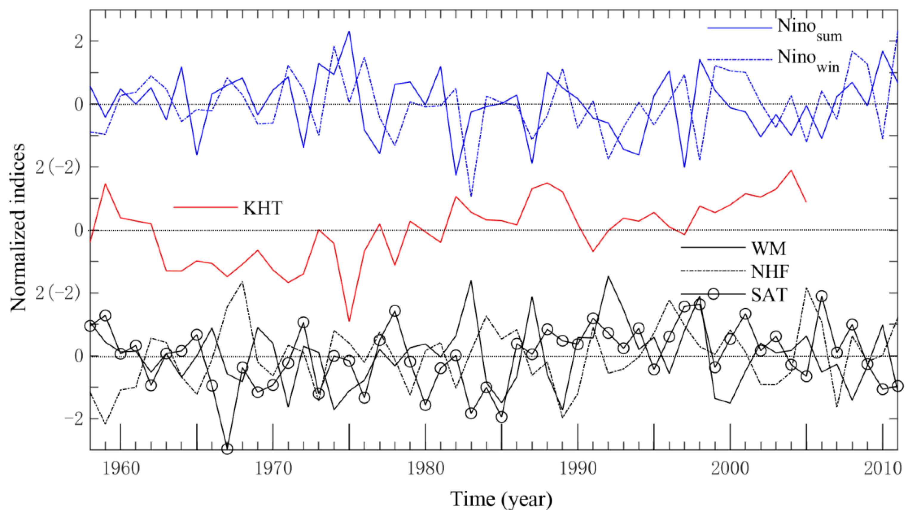
3.1.1. Local Forcings

Li et al. [27] demonstrated that local heat flux and wind stress in winter both affect YSCWM intensity. Zhu et al. [28] also showed that air–sea heat flux is the dominant factor influencing YSCWM intensity. Park et al. [21] reported that YSCWM intensity is associated with SAT. Li [43] showed that YSCWM intensity is also affected by KHT. Therefore, we examined the effects of the local WM, sea surface NHT, SAT, and KHT (Figure 6) on SYSCWM intensity. The correlation coefficients and corresponding p-values between SYSCWM intensity and those factors are shown in Figure 7.

It can be seen from Figure 7 that the T-10 index has positive correlation with the WM with a 1-year lead time, which suggests that a strong WM could reduce the temperature of the SYSCWM. Owing to the shallow depth of the YS, a strong WM can strengthen mixing and heat loss that both act to cool the bottom water in the YS trough. During the summer, this low-temperature water is maintained by the thermocline. Previous studies identified two different roles of the WM. For example, Kim and Kimura [44] revealed that strong northerly winds introduce a large vertical temperature difference at the air–sea interface, which produces a large amount of heat loss from the ocean. Conversely, both Hsueh and Yuan [45] and Moon et al. [46] showed that the increase in sea level induced by the northerly monsoon generates inflow of warm salty water from the YSWC, which might reduce the area of the YSCWM in the following summer [25,47]. Here, based on correlation analysis that indicates that the cooling effect of the WM is greater than the heating effect, we conclude that the WM can cool the SYSCWM. Wei et al. [30] also reported that during the cooling season, the lateral heat transport from the YSWC is about five times smaller than that of the net surface heat loss integrated over the YS.

Figure 8 shows the first SVD mode of the WM–SYSCWM fields, which accounts for 94% of their covariance (

Table 1. First SVD mode of ENSO and SYSCWM.

	Fraction of Covariance (%)	Correlation Coefficient of Time-Series
WM−SYSCWM	92	0.48
NHF-SYSCWM	89	0.56
SAT-SYSCWM	99	0.78
ENSOsum-WM	79	0.50
ENSOsum-SYSCWM	68	0.38
ENSOwin-NHF	84	0.43
WM−NHF	93	0.62

). As the spatial pattern of the SVD resembles the heterogeneous correlation pattern, we only provide the latter (and the same is true below). The heterogeneous correlation (Figure 8a) is high in the SYSCWM, indicating that a cold event in the SYSCWM is associated with a strong WM (Figure 8b); the correlation coefficient of the normalized time series of the first spatial pattern (Figure 8c) is 0.48. This coefficient is different from that in Figure 7. That is because the correlation coefficient in Figure 7 is obtained by the two original fields, while the coefficient here is the correlation of the time series from the high correlation modes of the two original fields.

The T-10 index has negative correlation with sea surface NHF at a 1-year lead time (Figure 7), which suggests that strong winter heat loss from the ocean to the atmosphere can cool the SYSCWM.

The T-10 index has positive correlation with SAT at a 1-year lead time (Figure 7), indicating that higher SAT in the previous winter can warm the SYSCWM.

The positive correlation between T-10 and winter KHT at a 1-year lead time (Figure 7) suggests that large KHT can warm the SYSCWM.

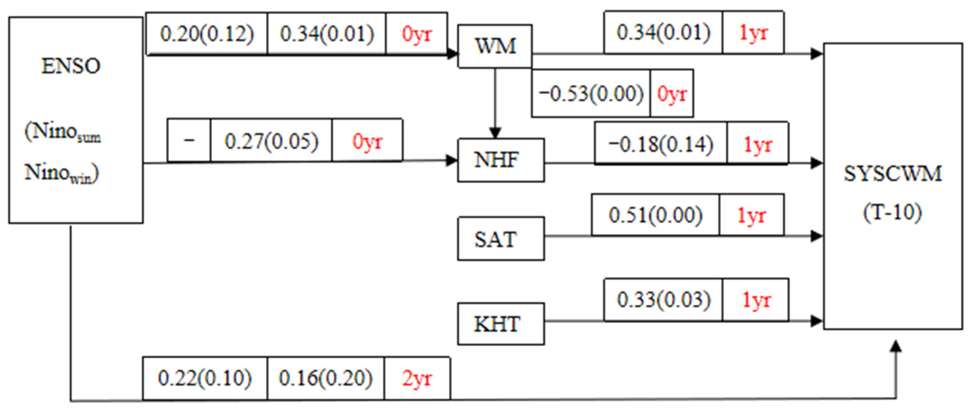
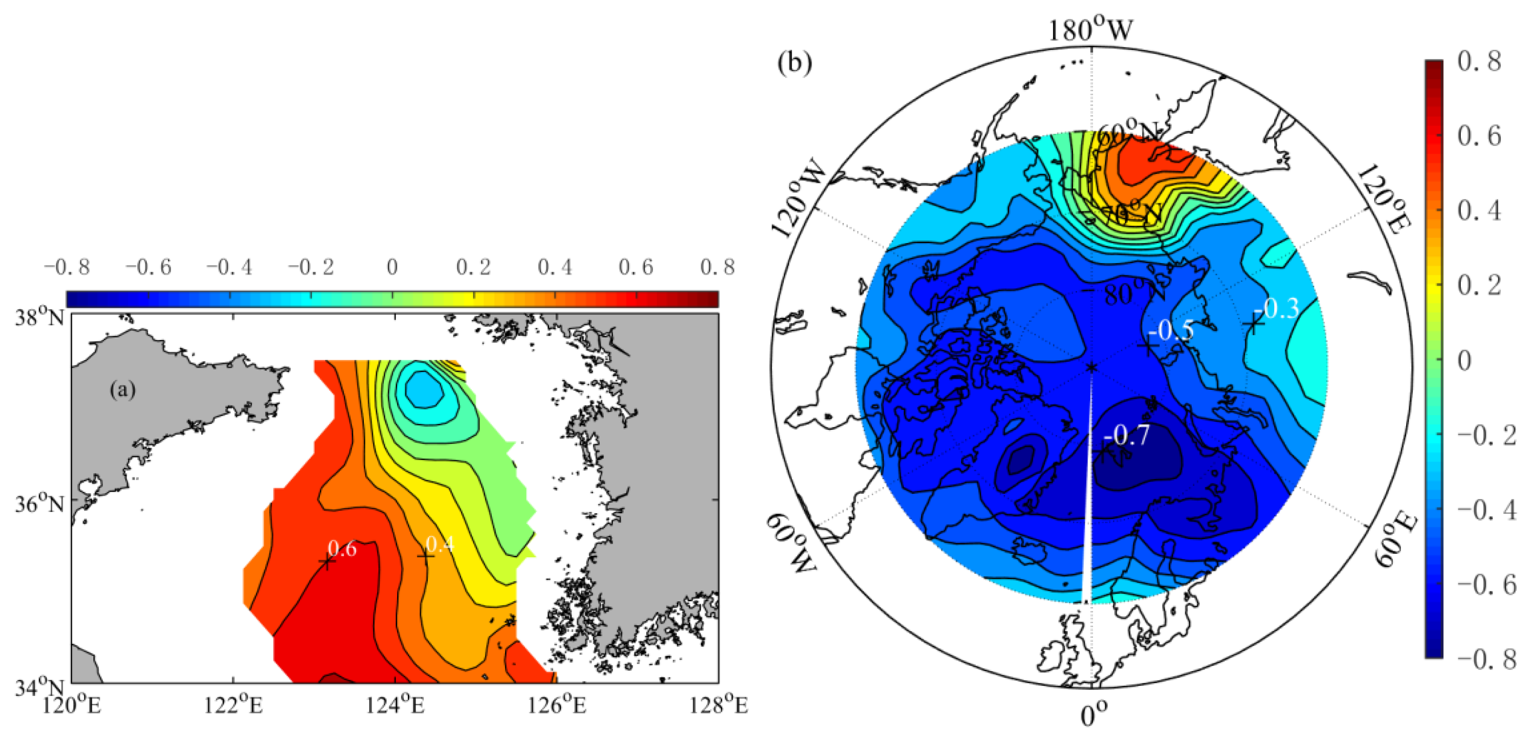
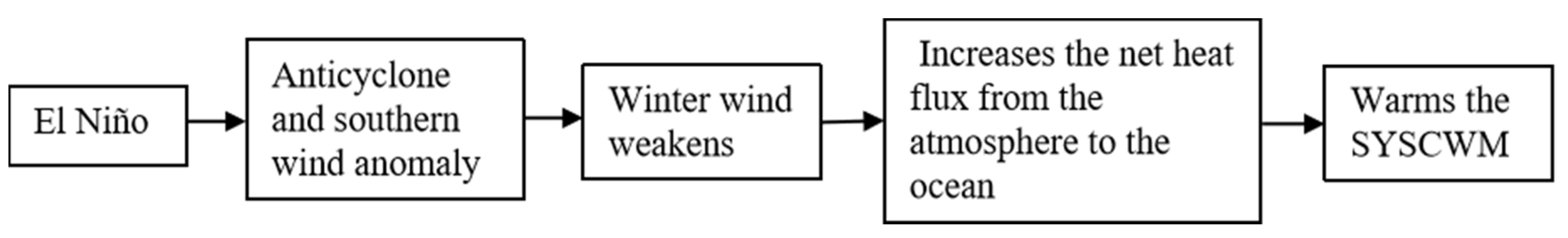
3.1.2. Effect of ENSO

We investigated the correlation between local factors and the ENSO index, as shown in Figure 7 and Table 1. The Nino3.4 index is well correlated synchronously with the WM. Positive correlation indicates that El Niño (La Niña) events correspond to a weak (strong) WM. A positive phase of ENSO can lead to the development of an anticyclone and southern wind anomaly in the lower troposphere of the western Pacific Ocean, weakening the winter wind.

The Nino3.4 index is also related to the T-10 index at a 2-year lead time, as shown in Figure 7. The correlation coefficients indicate that the SYSCWM is colder (warmer) during La Niña (El Niño) events, consistent with the results of the EOF analysis discussed in Section 3.1. Figure 9 presents the first SVD mode of the summer tropical SLP–SYSCWM fields, which accounts for 68% of their covariance (Table 1). The heterogeneous correlation in Figure 9a is high in the SYSCWM, while that in Figure 9b shows the ENSO mode, indicating that a colder event in the SYSCWM is associated with La Niña; the correlation coefficient of the normalized time series is 0.38 (Figure 9c). From the correlation between ENSO, WM, and the SYSCWM, we can conclude that ENSO can affect SYSCWM intensity via the local WM.

The negative correlation between the Nino3.4 index and sea surface NHF (Figure 7) suggests that during El Niño events, the NHF is from the atmosphere to the ocean, which can warm the SYSCWM. This prompts the question of how ENSO is related to the local sea surface NHF. It can be seen from Figure 7 that the winter NHF is affected by the local winter wind (correlation coefficient of −0.53) on a synchronous timescale. The correlation and SVD analysis indicate that a stronger winter wind contributes to a large amount of heat loss from the ocean to the atmosphere, and the local winter wind is affected by ENSO.

Table 1 shows the SVD analysis among other variables. Due to the space limitation of this paper, the modal diagrams are not listed one by one, but the results of these SVD analysis are consistent with the correlation analysis (Figure 7).

3.2. Decadal Variability of SYSCWM

In addition to the remarkable interannual variability of the SYSCWM, its decadal variation is also significant. Previous studies [21,27] have examined how both the PDO and the AO, which are the most significant decadal oscillations in the Pacific and Eurasian regions, might affect the YSCWM. In addition to the WM, NHF, SAT, and KHT described in Section 3.1, the lateral transport of heat into the YS via the YSWC also affects the SYSCWM. As is well known, the WM is always affected by the East Asian WM, which is controlled by the MH and AL. The PDO has strong correlation with the AL in winter [21,27,48] and the AO is well correlated with the MH [21,49]. Therefore, both the MH and the AL are considered as intermediate factors that affect the SYSCWM.

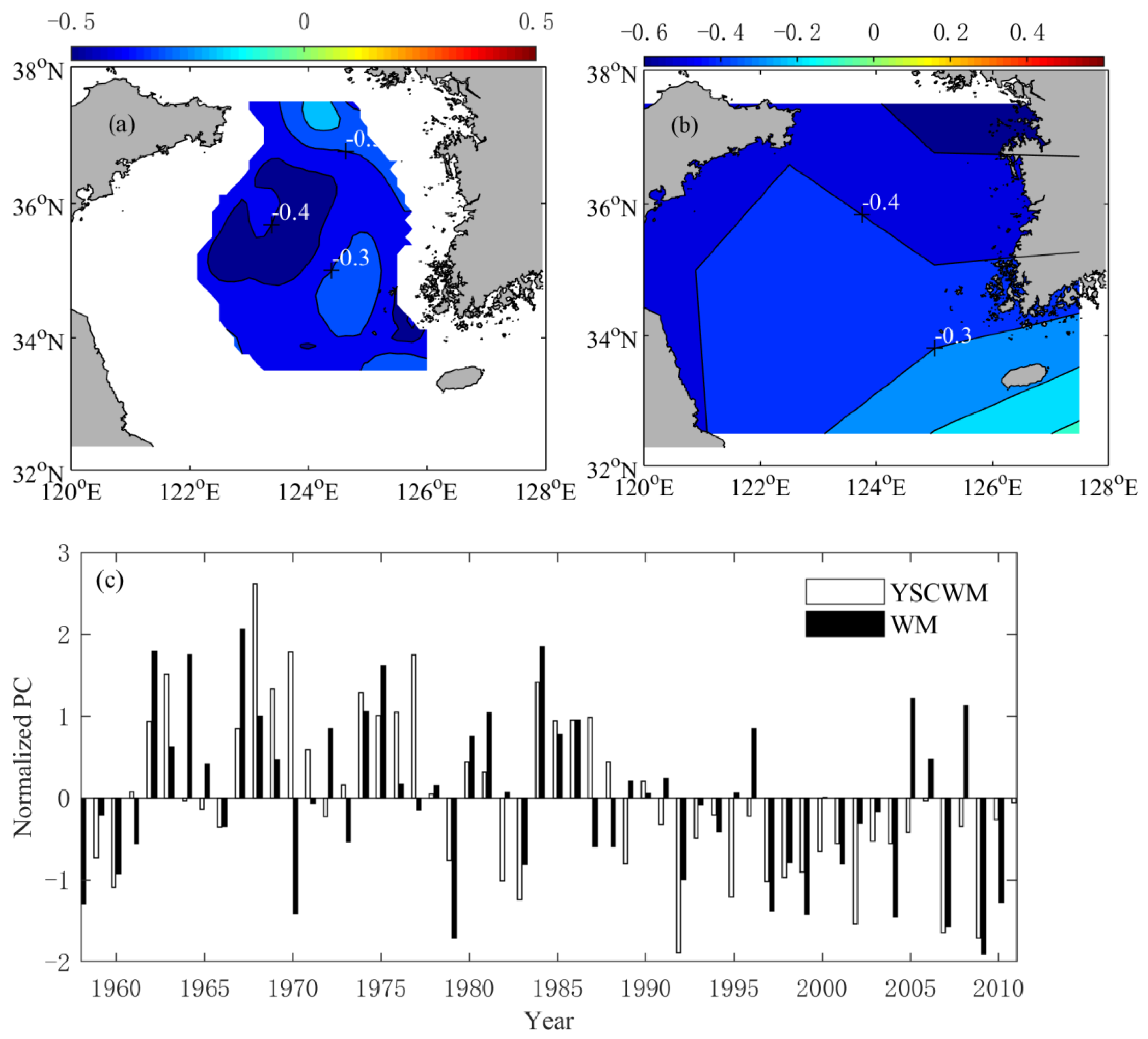
3.2.1. Local or Intermediate Forcings

The various indices after 7-year low-pass filtering are shown in Figure 10.

Figure 11 shows the correlation coefficients and corresponding p-values between the decadal variability of the SYSCWM and various forcing factors.

Table 2. First SVD mode of PDO/AO and SYSCWM.

	Fraction of Covariance (%)	Correlation Coefficient of Time-Series
MH-SYSCWM	51	0.67
MH-WM	84	0.52
AL-SYSCWM	88	0.49
AL-WM	51	0.47
KHT- SYSCWM	90	0.61
PDOwin-SYSCWM	85	0.76
PDOsum-WM	70	0.50
PDOsum-SAT	88	0.49
PDOwin-AL	65	0.72
PDOwin-KHT	54	0.46
AOwin-SYSCWM	92	0.65
AOwin-WM	87	0.35
AOwin-SAT	95	0.52
WM−SAT	96	0.57
WM−KHT	84	0.39

shows the SVD analysis of different factors and the results of these SVD analysis are consistent with the correlation analysis (Figure 11).

It can be seen that the WM/SAT has good positive correlation with the T-10 index at a 2-year lead time, and that sea surface NHF is correlated negatively with the T-10 index at a 2-year lead time. The mechanism via which the WM, NHF, and SAT influence the SYSCWM was explained in Section 3.1.

Winter KHT has strong positive correlation with the T-10 index at a 2-year lead time (Figure 11), which suggests that substantial KHT can warm the SYSCWM. Because ocean analysis data have good spatiotemporal coverage, we downloaded the northward current velocity data of the PN section from the CORA dataset and calculated the velocity anomaly, which represents the variation of KHT [31]. The first SVD mode of the winter northward current velocity–SYSCWM fields (Figure 12), which accounts for 90% of their covariance (Table 2), also indicates that a warmer event in the SYSCWM is associated with larger KHT. The YSWC has positive correlation with the T-10 index (Figure 11), which can be explained by the greater lateral transport of heat into the YS when the winter intrusion of the YSWC is enhanced. The correlation coefficient between the intensity of the YSWC and the winter KHT is 0.38 (Figure 11), which suggests that substantial KHT can strengthen the YSWC. Tang et al. [41] verified that the YSWC represents mixing of the northward Kuroshio branch and the shelf water of the East China Sea. Thus, we conclude that the Kuroshio can affect the SYSCWM through the YSWC.

The MH is correlated negatively with the T-10 index at a 3-year lead time (Figure 11), which means the stronger the MH, the colder the SYSCWM. The correlation coefficient between the MH and WM is −0.43 on a synchronous timescale (Figure 11), meaning that a strong MH can strengthen the local winter wind in the YS. Because the MH has negative correlation with the WM and the WM has positive correlation with the T-10 index, the MH has negative correlation with T-10 index. Thus, we conclude that the MH influences the SYSCWM through the local winter wind.

The AL is negatively connected with the T-10 index at a 3-year lead time (Figure 11), which means a stronger AL is associated with a warmer SYSCWM. As is well known, a barometric field is always connected to the wind field. The correlation coefficient between the AL and the WM is −0.36 at a 2-year lead time (Figure 11), which means a strong AL can weaken the local winter wind in the YS. The AL also affects the SYSCWM through the local winter wind. The reason why the AL and the WM are correlated negatively will be explained in Section 3.2.2.

For the above forcing factors, the correlation coefficients of the WM, SAT, and KHT with the SYSCWM are the highest (Figure 11), meaning the WM, SAT, and KHT play the most important roles in the decadal variation of SYSCWM intensity.

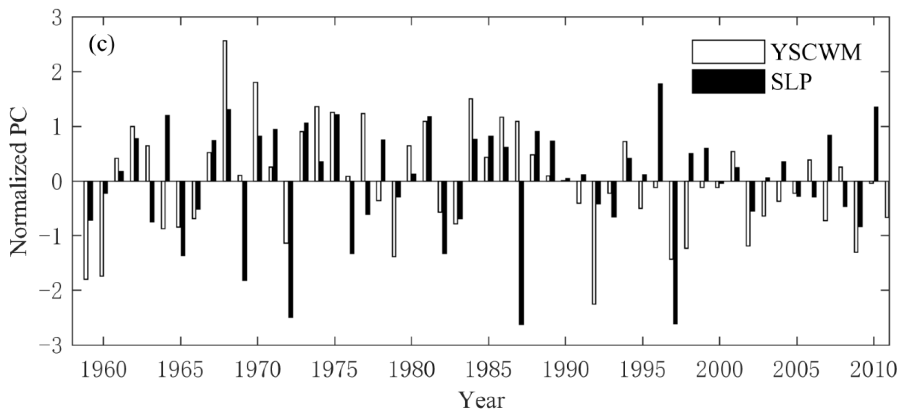
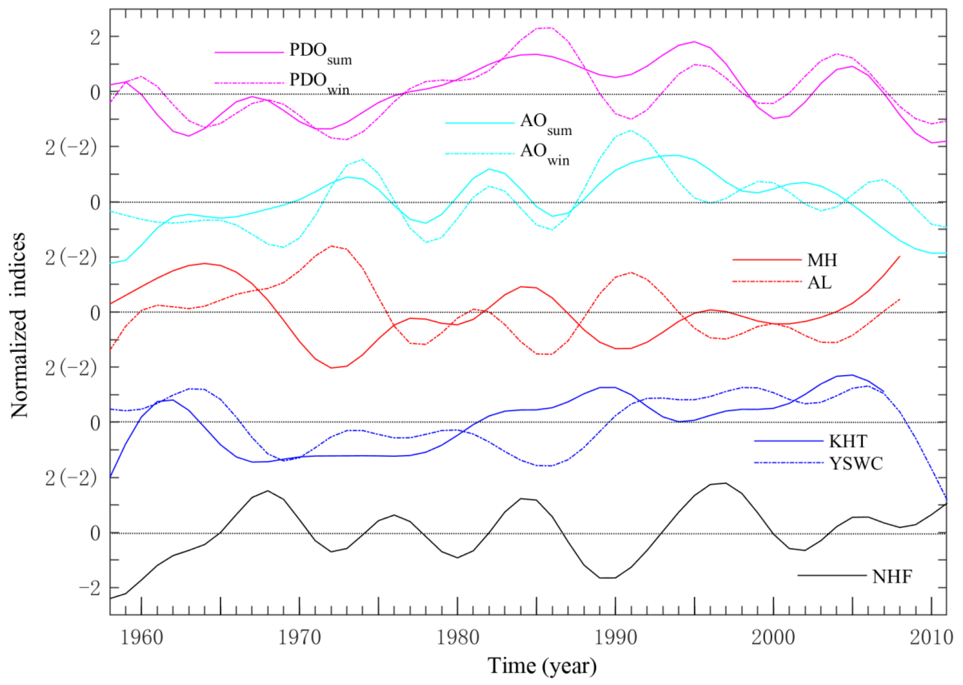
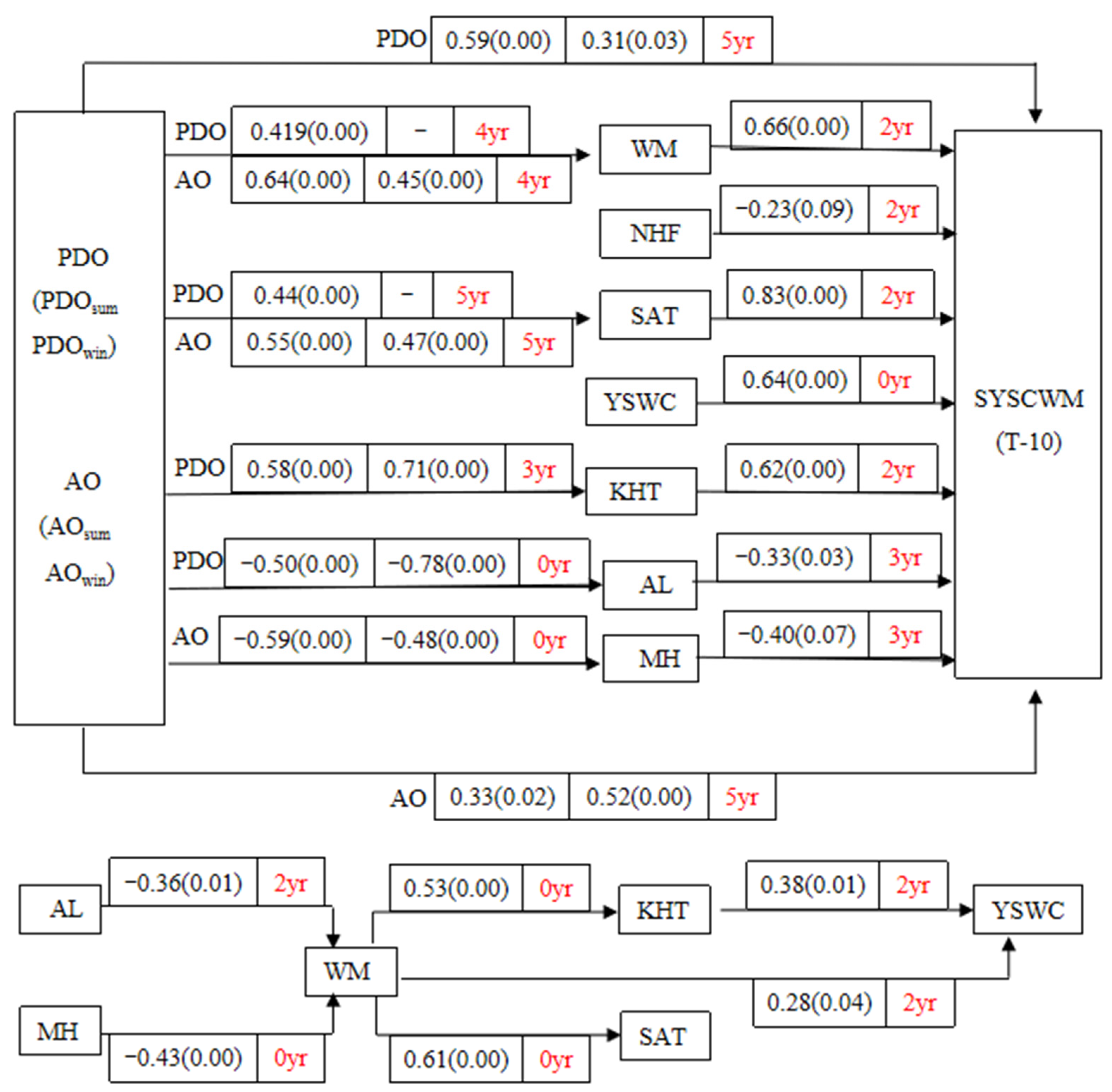
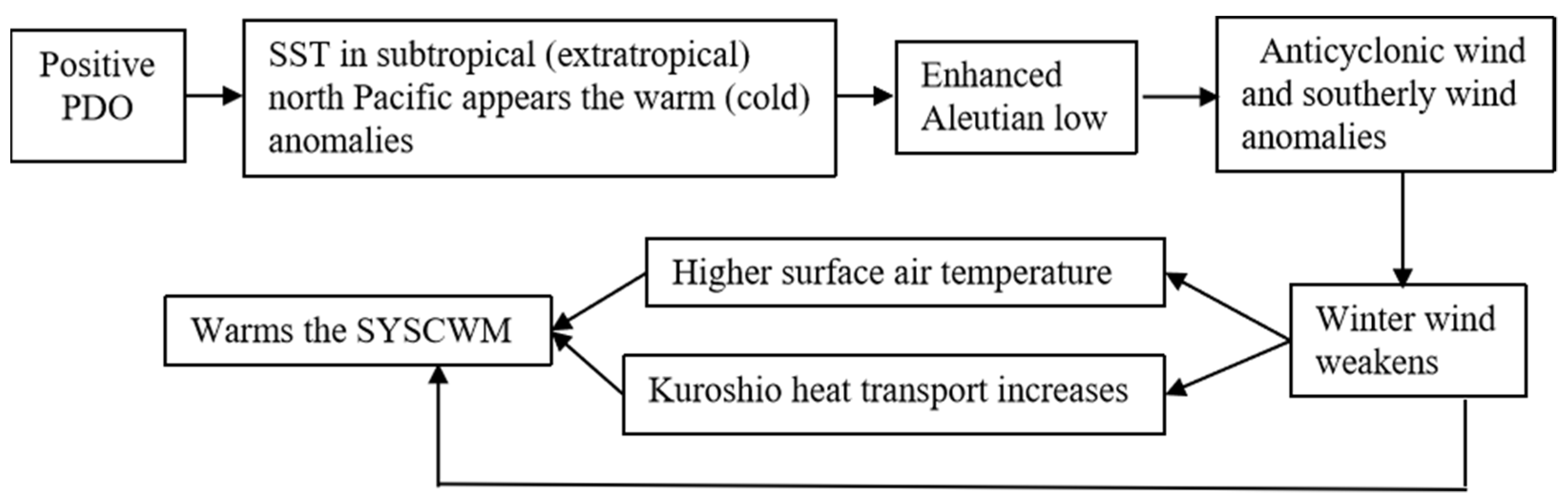
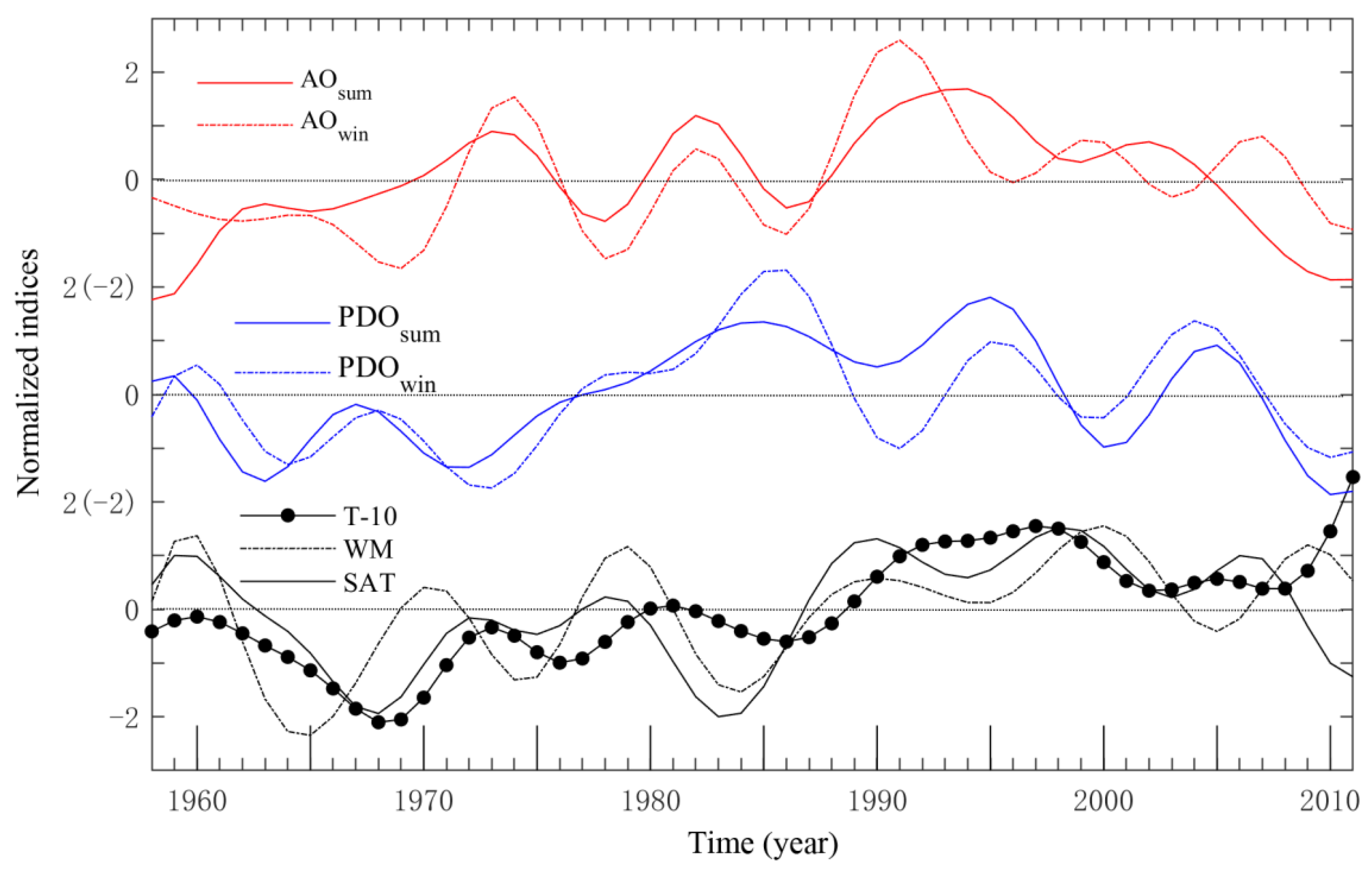
3.2.2. Remote Forcings

We examined the correlation coefficients between the PDO/AO and local or intermediate factors, as shown in Figure 11.

The PDO has strong negative correlation with the AL on a synchronous timescale (Figure 11), implying that the AL is enhanced when the PDO is in its positive phase. When the PDO is in its positive phase, the SST in the subtropical North Pacific Ocean appears as a warm anomaly. Therefore, the AL is enhanced and the pressure over the subtropical North Pacific Ocean is also enhanced. This SST and pressure distribution contributes to the anticyclonic wind over the eastern Philippines, which produces a southerly wind anomaly in southern China. In winter, this southerly wind anomaly can weaken the prevailing northerly monsoon, which explains why both the AL and the WM are correlated negatively, as mentioned above. As the PDO is correlated negatively with the AL, the AL is in turn negatively associated with the WM. Therefore, the PDO should be correlated positively with the WM, as is shown in Figure 11 with a correlation coefficient of 0.41 at a 4-year lead time.

The PDO has strong positive correlation with KHT at a 3-year lead time (Figure 11), implying that when the PDO is in its positive phase, KHT is enhanced. The PDO can affect the WM and the WM is related to KHT with a correlation coefficient of 0.53 at a synchronous timescale (Figure 11). Both Zhang et al. [31] and Qi et al. [50] have proven that a strong WM will reduce KHT. Thus, we believe that the PDO is connected to KHT through the WM. As mentioned in Section 3.2.1, KHT is correlated positively with the YSWC. Therefore, the WM should be correlated positively with the YSWC through KHT. However, both Hsueh and Yuan [45] and Moon et al. [46] showed that the increase in sea level induced by a northerly strong monsoon generates inflow of warm salty water from the YSWC. Therefore, the WM should be correlated negatively with the YSWC. We calculated the correlation between the WM and YSWC. The resultant positive correlation (Figure 11) indicates that the effect of the WM on the YSWC through KHT is greater than that through the sea level.

The AO has strong negative correlation with the MH at a synchronous timescale (Figure 11), indicating that the MH is weakened when the AO is in its positive phase. The positive phase of the AO corresponds to decreasing pressure in the polar region, which can strengthen the zonal wind of the upper atmosphere at mid- and high latitudes. This means the East Asian trough is filled and the convergence and descent at the rear of the trough is diminished; thus, the surface MH is weakened. The MH can affect the East Asian winter monsoon and further affect the local winter wind over the YS. The correlation coefficient between the MH and WM is −0.43 at a synchronous timescale (Figure 11), suggesting that the local winter wind is stronger when the MH is stronger. As the AO is correlated negatively with the MH and the MH is in turn correlated negatively with the WM, the AO should be correlated positively with the WM, as shown in Figure 11.

The PDO and AO both have strong positive correlation with SAT (Figure 11). As is well known, when the WM is strengthened, strong cold air breakouts are common. The correlation coefficient between the WM and SAT is 0.61 at a synchronous timescale (Figure 11), implying that a strong WM can cool sea surface air. The PDO and AO both have positive correlation with the WM and the WM has positive correlation with SAT, which explains the positive correlation between the PDO/AO and SAT.

Through the above analysis, we find that the PDO and AO can ultimately act on the WM.

The direct correlation between the PDO/AO and SYSCWM intensity is shown in Figure 11. The PDO has strong positive correlation with the T-10 index at a 5-year lead time, implying that when the PDO is in its positive phase, the SYSCWM is warmer. Figure 13 shows the first SVD mode between the winter northern Pacific SST and SYSCWM, which accounts for 85% of their covariance (Table 2). The heterogeneous correlation shown in Figure 13b, which is high in the central North Pacific Ocean, reflects the PDO mode. Thus, we can conclude that when the PDO is in its cold phase, the SYSCWM is colder.

The AO is correlated positively with the T-10 index at a 5-year lead time (Figure 11), implying that the SYSCWM is warmer when the AO is in its positive phase. The first SVD mode between the winter SLP in the Arctic (representing the AO mode) and the SYSCWM (Figure 14) also verifies this.

4. Discussion

Based on the analysis from Section 3.1, we can conclude that ENSO affects the WM, the WM affects the sea surface NHF, and the sea surface NHF affects the SYSCWM. A schematic of the “forcing mechanism bridge” via which El Niño can affect the SYSCWM is shown in Figure 15 and that of La Niña is the contrary.

Li [33] indicated that ENSO is connected with KHT and we also found that both ENSO and KHT are related to the YSCWM; however, we did not find significant correlation between ENSO and KHT on the interannual timescale, which is a subject that might require further study.

By combining the discussions in Section 3.2, we can conclude there are two “forcing mechanism bridges” via which the remote PDO can affect SYSCWM intensity on the decadal timescale:$\mathrm{PDO}\stackrel{-}{\to }\mathrm{AL}\stackrel{-}{\to }\mathrm{WM}\stackrel{+}{\to }\mathrm{SAT}\stackrel{+}{\to }\mathrm{SYSCWM}$ and $\mathrm{PDO}\stackrel{-}{\to }\mathrm{AL}\stackrel{-}{\to }\mathrm{WM}\stackrel{+}{\to }\mathrm{KHT}\stackrel{+}{\to }\mathrm{YSWC}\stackrel{+}{\to }\mathrm{SYSCWM}$ (where the “+” and “−” above the arrow means positive and negative correlation, respectively). Based on logical operation of the positive and negative correlations, the PDO is ultimately correlated positively with the temperature of the SYSCWM via both pathways, as shown in Figure 11. The schematic of the pathway (Figure 16) through which the PDO affects the SYSCWM reflects a period when PDO is in its positive phase.

Other pathways via which the PDO might affect the YSCWM have been reported in other studies. For example, Li et al. [27] indicated that when the PDO is in its positive phase, the heat flux from the atmosphere to ocean is increased in the YS, which reduces the area of the YSCWM. We verified that the sea surface NHF is associated with SYSCWM intensity, but we did not find evidence of a significant relationship between the PDO and NHF. Both Jiang et al. [24] and Li [51] found that the Kuroshio Meander always induces a warmer YSCWM in the following year. This is because the large meander of the Kuroshio always corresponds to large volume/heat transport of the Kuroshio [52,53] Based on the relationship between KHT and the SYSCWM revealed in Section 3.2.1, we can confirm that the large meander of the Kuroshio does warm the SYSCWM.

The “forcing mechanism bridges” via which the remote AO affects the SYSCWM are presented in Figure 17. The schematic of this pathway reflects a period when the AO is in its positive phase.

The normalized time series of the AO, PDO, T-10, WM, and SAT smoothed by 7-year low-pass filtering are shown in Figure 18. Around 1980, both the PDO and the AO change from negative to positive phase. Correspondingly, the WM and SAT exhibit the same phase transition, which means the WM becomes weaker and SAT becomes higher. Many other indices of the East Asian WM have indicated its decadal-scale weakening since the mid-1980s; it is the most prominent characteristic over the previous 100 years. After 1980, the SYSCWM also becomes warmer. Therefore, the consistent phase change of both the PDO and the AO contributes to the significant decadal variability of SYSCWM intensity.

Based on the above analysis, we conclude that the decadal variation of SYSCWM intensity is controlled mainly by the WM, SAT, summer PDO, and winter AO. This encouraged us to infer SYSCWM intensity by establishing a simple equation using these factors, which could be helpful in predicting the approximate decadal variability of SYSCWM intensity. If additional factors were used in the multiple regression analysis, the regression coefficient of some factors would be opposite to the correlation coefficient in the correlation analysis, which is against physical principles. Through the test of regression analysis, we found that the correlation coefficient R² of the regression analysis remained largely unchanged irrespective of whether SAT is considered. In addition, SAT has strong correlation with the WM; therefore, we opted to use the WM, PDO_sum, and AO_win to construct the equation. Through the multiple regression analysis, the formula (which passed the F-test at the 95% confidence level) for predicting the T-10 (°C, R² = 0.72) is as follows:

$$\mathrm{T}-10=9.821+0.105\mathrm{WM}+0.061{\mathrm{PDO}}_{\mathrm{sum}}+0.035{\mathrm{AO}}_{\mathrm{win}}$$

(1)

The regression coefficients in Equation (1) suggest that the effect on the SYSCWM is WM > PDO > AO. The reconstructed time series of T-10 during 1958–2011 (circles in Figure 19) are compared with the original data (dots in Figure 19). The correlation coefficients between the original and reconstructed data are 0.83, with a significance level of 95%. In addition, we predicted the T-10 from 2012 to 2018 based on Equation (1), and compared the results with the reanalysis data from the National Marine Data Center (http://mds.nmdis.org.cn/pages/home.html, accessed on 17 November 2021), as shown in the red line in Figure 19. The comparison results verify the Equation (1). Thus, the decadal variation of the SYSCWM is effectively captured by these factors.

5. Conclusions

This study used CORA data to investigate the low-frequency variability of the SYSCWM. We explored the mechanisms via which the remote forcings affect SYSCWM intensity through local or intermediate forcings. On the interannual timescale, ENSO can affect the SYSCWM through the local WM and sea surface NHF. On the decadal timescale, the PDO affects the SYSCWM via two “bridges”: $\mathrm{PDO}\stackrel{-}{\to }\mathrm{AL}\stackrel{-}{\to }\mathrm{WM}\stackrel{+}{\to }\mathrm{SAT}\stackrel{+}{\to }\mathrm{SYSCWM}$ and $\mathrm{PDO}\stackrel{-}{\to }\mathrm{AL}\stackrel{-}{\to }\mathrm{WM}\stackrel{+}{\to }\mathrm{KHT}\stackrel{+}{\to }\mathrm{YSWC}\stackrel{+}{\to }\mathrm{SYSCWM}$. The “forcing mechanism bridge” via which the AO affects the SYSCWM is $\mathrm{AO}\stackrel{-}{\to }\mathrm{MH}\stackrel{-}{\to }\mathrm{WM}\stackrel{+}{\to }\mathrm{SAT}\stackrel{+}{\to }\mathrm{SYSCWM}$. Through analysis of climate change, we concluded that before and after the 1980s, the consistent phase change of the PDO and the AO has contributed to the significant decadal variability of the SYSCWM. Finally, we established one simple formula for predicting the decadal variability of SYSCWM intensity using the key influencing factors.

It should be noted that the atmospheric models such as NCEP has a tendency to underestimate short wave gain and overestimate the long wave loss [54]. When using NCEP data to construct climate factors for correlation analysis, it may have an impact on the magnitude of the correlation coefficient and the determination of lag/lead time. Because the interaction and the response between the ocean and the atmosphere takes time, the correlation between different climate factors has lead/lag time. The analysis of the impact of input data and the causes of lag/lead time in this paper will be our next work.

References

1. He, C.B.; Wang, Y.X.; Lei, Z.Y.; Xu, S. A preliminary study of the formation of Yellow Sea cold mass and its properties. Oceanol. Limnol. Sin. 1959, 2, 11–15. (In Chinese) [Google Scholar]
2. Chen, Y.L.; Hu, D.X.; Wang, F. Long-term variabilities of thermodynamic structure of the East China Sea Cold Eddy in Summer. J. Oceanol. Limnol. 2004, 22, 224–230. [Google Scholar] [CrossRef]
3. Lie, H.-J.; Cho, C.-H.; Lee, J.-H.; Lee, S.; Tang, Y.; Zou, E. Does the yellow sea warm current really exist as a persistent mean flow? J. Geophys. Res. Oceans 2001, 106, 22199–22210. [Google Scholar] [CrossRef]
4. Hur, H.B.; Jacobs, G.A.; Teague, W.J. Monthly variations of water masses in the Yellow and East China Seas, November 6, 1998. J. Oceanogr. 1999, 55, 171–184. [Google Scholar] [CrossRef]
5. Horsburgh, K.J.; Hill, A.E.; Brown, J.; Fernand, L.; Garvine, R.W.; Angelico, M.M.P. Seasonal evolution of the cold pool gyre in the western Irish Sea. Prog. Oceanogr. 2000, 46, 1–58. [Google Scholar] [CrossRef]
6. Yu, X.; Guo, X.; Takeoka, H. Fortnightly variation in the bottom thermal front and associated circulation in a semienclosed sea. J. Phys. Oceanogr. 2016, 46, 159–177. [Google Scholar] [CrossRef]
7. Li, H.B.; Xiao, T.; Ding, T.; Lu, R. Effect of the Yellow Sea Cold Water Mass (YSCWM) on distribution of bacterioplankton. Acta Ecol. Sin. 2006, 26, 1012–1019. [Google Scholar] [CrossRef]
8. Wang, D.; Huang, B.Q.; Liu, X.; Lu, G.; Wang, H. Seasonal variations of phytoplankton phosphorus stress in the Yellow Sea Cold Water Mass. Acta Oceanol. Sin. 2014, 33, 124–135. [Google Scholar] [CrossRef]
9. Liu, X.; Huang, B.Q.; Huang, Q.; Wang, L.; Ni, X.; Tang, Q.; Song, S.; Hao, W.; Liu, S.; Li, C.; et al. Seasonal phytoplankton response to physical processes in the southern Yellow Sea. J. Sea Res. 2015, 95, 45–55. [Google Scholar] [CrossRef]
10. Xin, M.; Ma, D.Y.; Wang, B.D. Chemicohydrographic characteristics of the Yellow Sea Cold Water Mass. Acta Oceanol. Sin. 2015, 34, 5–11. [Google Scholar] [CrossRef]
11. Wang, B.; Hirose, N.; Kang, B.; Takayama, K. Seasonal migration of the Yellow Sea Bottom Cold Water. J. Geophys. Res. Oceans 2015, 119, 4430–4443. [Google Scholar] [CrossRef]
12. Wang, R.; Zuo, T.; Wang, K. The Yellow Sea cold bottom water-an oversummering site for Calanus sinicus (Copepoda, Crustacea). J. Plankton Res. 2003, 25, 169–183. [Google Scholar] [CrossRef] [Green Version]
13. Cho, K.D. On the influence of the Yellow Sea Bottom Cold Water on the demersal fishing grounds. J. Korean Soc. Fish. Technol. 1982, 18, 25–33. [Google Scholar]
14. Du, B.; Zhang, Y.J.; Shan, Y.C. The characteristics of cold water mass variation at the bottom of the North Yellow Sea and its hydrological effects on the mortality of shellfish cultured in the waters of outer Changshun Islands. Mar. Sci. Bull. 1996, 15, 17–28, (In Chinese with English abstract). [Google Scholar]
15. Wan, B.J.; Guo, B.H.; Chen, Z.S. A three-layer model for the thermal structure in the Huanghai Sea. Acta Oceanol. Sin. 1990, 9, 159–172. [Google Scholar]
16. Miu, J.B.; Liu, X.Q.; Xue, Y. The preliminary discussion of the formation mechanism of the north Yellow Sea Cold Water Mass-II. Discussion of model solution. Sci. China 1991, 21, 74–81. (In Chinese) [Google Scholar] [CrossRef]
17. Chu, P.C.; Wells, S.K.; Haeger, S.D.; Szczechowski, C.; Carron, M. Temporal and spatial scales of the Yellow Sea thermal variability. J. Geophys. Res. Oceans 1997, 102, 5655–5667. [Google Scholar] [CrossRef] [Green Version]
18. Hu, D.X.; Wang, Q.Y. Interannual variability of the southern Yellow Sea cold water mass. Chin. J. Oceanol. Limnol. 2004, 22, 231–236. [Google Scholar] [CrossRef]
19. Yu, F.; Zhang, Z.X.; Diao, X.Y. Analysis of evolution of the Huanghai Sea Cold Water Mass and its relationship with adjacent water masses. Acta Oceanol. Sin. 2006, 28, 26–34, (In Chinese with English abstract). [Google Scholar]
20. Zhang, S.W.; Wang, Q.Y.; Lu, Y.; Cui, H.; Yuan, Y.L. Observation of the seasonal evolution of the Yellow Sea Cold Water Mass in 1996–1998. Cont. Shelf Res. 2008, 28, 442–457. [Google Scholar] [CrossRef]
21. Park, S.; Chu, P.C.; Lee, J.H. Interannual-to-interdecadal variability of the Yellow Sea Cold Water Mass in 1967–2008: Characteristics and seasonal forcings. J. Mar. Syst. 2011, 87, 177–193. [Google Scholar] [CrossRef] [Green Version]
22. Yuan, Y.L.; Li, H.Q. Theoretical study on the circulation structure and the formation mechanisms related to cold water mass of Yellow Sea- I. The zero order solution and circulation structure of cold water mass. Sci. China 1993, 23, 93–103. (In Chinese) [Google Scholar]
23. Ren, H.J.; Zhan, J.M. A numerical study on the seasonal variability of the Yellow Sea cold water mass and the related dynamics. J. Hydrodyn. 2005, 20 (Suppl. 1), 887–896. [Google Scholar] [CrossRef]
24. Jiang, B.J.; Bao, X.W.; Wu, D.X.; Xu, J.P. Interannual variation of temperature and salinity of northern Huanghai Sea Cold Water Mass and its probable cause. Acta Oceanol. Sin. 2007, 29, 1–10. [Google Scholar] [CrossRef]
25. Wei, H.; Shi, J.; Lu, Y.Y.; Peng, Y. Interannual and long-term hydrographic changes in the Yellow Sea during 1977–1998. Deep-Sea Res. Part II Top. Stud. Oceanogr. 2010, 57, 1025–1034. [Google Scholar] [CrossRef]
26. Yang, H.W.; Cho, Y.K.; Seo, G.H.; You, S.H.; Seo, J.W. Interannual variation of the southern limit in the Yellow Sea Bottom Cold Water and its causes. J. Mar. Syst. 2014, 139, 119–127. [Google Scholar] [CrossRef]
27. Li, X.W.; Wang, X.D.; Chu, P.C.; Zhao, D. Low-frequency variability of the Yellow Sea Cold Water Mass identified from the China coastal waters and adjacent seas reanalysis. Adv. Meteorol. 2015, 2015, 269859. [Google Scholar] [CrossRef] [Green Version]
28. Zhu, J.Y.; Shi, J.; Guo, X.Y.; Guo, H.; Yao, X. Air-sea heat flux control on the Yellow Sea Cold Water Mass intensity and implications for its prediction. Cont. Shelf Res. 2018, 152, 14–26. [Google Scholar] [CrossRef]
29. Han, G.J.; Li, W.; Zhang, X.F.; Li, D.; He, Z.; Wang, X.; Wu, X.; Yu, T.; Ma, J. A regional ocean reanalysis system for coastal waters of China and adjacent seas. Adv. Atmos. Sci. 2011, 28, 682–690. [Google Scholar] [CrossRef]
30. Wei, H.; Yuan, C.Y.; Lu, Y.Y.; Zhang, Z.; Luo, X. Forcing mechanisms of heat content variations in the Yellow Sea. J. Geophys. Res. Oceans 2013, 118, 4504–4513. [Google Scholar] [CrossRef]
31. Zhang, Q.L.; Hou, Y.J.; Qi, Q.H.; Zheng, D.M.; Cheng, M.H. Variations in the Kuroshio heat transport in the East China Sea and meridional wind anomaly. Adv. Mar. Sci. 2008, 26, 126–134. (In Chinese) [Google Scholar]
32. Sun, X.J.; Wang, P.X.; Zhi, H.; Guo, D. Analysis and comparison of several Mongolian High circulation indices and their relationship with temperature anomaly of China in winter. Plateau Meteorol. 2010, 29, 1493–1500. (In Chinese) [Google Scholar]
33. Wang, P.X.; Wang, J.L.X.L.; Zhi, H.; Wang, Y.; Sun, Y. Circulation indices of the Aleutian Low pressure system: Definitions and relationships to climate anomalies in the northern hemisphere. Adv. Atmos. Sci. 2012, 29, 1111–1118. [Google Scholar] [CrossRef]
34. Kalnay, E.; Kanamitsu, M.; Kistler, R.; Collins, W.; Deaven, D. The NCEP/NCAR 40-year reanalysis project. Bull. Amer. Meteorol. Soc. 1996, 77, 437–472. [Google Scholar] [CrossRef] [Green Version]
35. McPhaden, M.J. TAO/TRITON tracks Pacific Ocean warming in early 2002. CLIVAR Exchanges 2002, 7, 7–9. [Google Scholar]
36. Minobe, S.; Sako, A.; Nakamura, M. Interannual to interdecadal variability in the Japan Sea based on a new gridded upper water temperature dataset. J. Phys. Oceanogr. 2004, 34, 2382–2397. [Google Scholar] [CrossRef] [Green Version]
37. Park, S.Y.; Chu, P.C. Interannual SST variability in the Japan/East Sea and relationship with environmental variables. J. Oceanogr. 2006, 62, 115–132. [Google Scholar] [CrossRef]
38. Park, Y.H. Water characteristics and movements of the Yellow Sea Warm Current in summer. Prog. Oceanogr. 1986, 17, 243–254. [Google Scholar] [CrossRef]
39. Isobe, A. The Taiwan–Tsushima Warm Current system: Its path and the transformation of the water mass in the East China Sea. J. Oceanogr. 1999, 55, 185–195. [Google Scholar] [CrossRef]
40. Lie, H.-J.; Cho, C.-H.; Lee, J.-H.; Lee, S.; Tang, Y. Seasonal variation of the Cheju Warm Current in the northern East China Sea. J. Oceanogr. 2000, 56, 197–211. [Google Scholar] [CrossRef]
41. Tang, Y.X.; Zou, E.M.; Lie, H.-J. On the origin and path of the Huanghai Warm Current during winter and early spring. Acta Oceanol. Sin. 2001, 23, 1–12, (In Chinese with English abstract). [Google Scholar]
42. Yu, F.; Zhang, Z.X.; Diao, X.Y.; Guo, J. Erratum to: Observational evidence of the Yellow Sea warm current. J. Oceanol. Limnol. 2010, 28, 954. [Google Scholar] [CrossRef] [Green Version]
43. Li, X.Y. A diagnostic study of 1998/2000 ENSO cold episode. J. Trop. Meteorol. 2001, 17, 90–96. [Google Scholar] [CrossRef]
44. Kim, Y.S.; Kimura, R. Estimation of the heat flux exchanges between the air-sea interface over the neighbouring seas of Korean Peninsula. J. Atmos. Sci. 1999, 35, 501–510. [Google Scholar]
45. Hsueh, Y.; Yuan, D.L. A numerical study of currents, heat advection, and sea-level fluctuations in the Yellow Sea in winter 1986. J. Phys. Oceanogr. 1997, 27, 2313–2326. [Google Scholar] [CrossRef]
46. Moon, J.H.; Hirose, N.; Yoon, J.H. Comparison of wind and tidal contributions to seasonal circulation of the Yellow Sea. J. Geophys. Res. Oceans 2009, 114, C08016. [Google Scholar] [CrossRef]
47. Ma, J.; Qiao, F.L.; Xia, C.S.; Kim, C.S. Effects of the Yellow Sea Warm Current on the winter temperature distribution in a numerical model. J. Geophys. Res. Oceans 2006, 111, C11S03. [Google Scholar] [CrossRef] [Green Version]
48. Zhu, Y.M.; Yang, X.Q. Relationships between Pacific Decadal Oscillation (PDO) and climate variabilities in China. Acta Meteorol. Sin. 2003, 61, 641–654, (In Chinese with English abstract). [Google Scholar]
49. Ding, Y.H.; Liu, Y.J.; Liang, S.J.; Ma, X.; Zhang, Y.; Liang, P.; Song, Y.; Zhang, J. Interdecadal variability of the East Asian winter monsoon and its possible links to global climate change. J. Meteorol. Res. 2014, 28, 693–713. [Google Scholar] [CrossRef]
50. Qi, J.F.; Yin, B.S.; Yang, D.Z.; Xu, Z. The inter-annual and inter-decadal variability of the Kuroshio volume transport in the East China Sea. Oceanol. Et Limnol. Sin. 2014, 45, 1141–1147, (In Chinese with English abstract). [Google Scholar]
51. Li, K.P. The response of the Yellow Sea Cold Water Mass on the ocean changes. Acta Oceanol. Sin. 1991, 13, 779–785. (In Chinese) [Google Scholar]
52. Liu, J.P.; Guan, B.X. Preliminary study of relation between the Kuroshio Meander and the El Nino event. Acta Oceanol. Sin. 1986, 8, 123–129. [Google Scholar]
53. Sun, X.P.; Wang, Y.P.; Yuan, Q.K.; Xuan, H. The variation of the Kuroshio during 1986–1988. Acta Oceanol. Sin. 1991, 10, 355–371. [Google Scholar]
54. Josey, S.A. A comparison of ECMWF, NCEP–NCAR, and SOC surface heat fluxes with moored buoy measurements in the subduction region of the Northeast Atlantic. J. Clim. 2001, 14, 1780–1789. [Google Scholar] [CrossRef]
Figure 1. Topography of the YS. The color contours denote bathymetry (m). The red solid line is the section A–B.
Jmse 09 01316 g001
Figure 2. Climatological temperature in the YS in July along 35° N from CORA data.
Jmse 09 01316 g002
Figure 3. The SYSCWM intensity index (°C) and the linear trend.
Jmse 09 01316 g003
Figure 4. Climatological monthly averaged temperature (°C) at the depth of 50 m in the YS from CORA data.
Jmse 09 01316 g004
Figure 5. Second EOF mode of the interannual components for temperature along the section A–B: (a) spatial mode, (b) smoothed temporal mode.
Jmse 09 01316 g005
Figure 6. Standardized indices of local WM, NHF, SAT, KHT and Nino3.4. Subscript sum (win) is the abbreviation of summer (winter).
Jmse 09 01316 g006
Figure 7. Correlation coefficients between the SYSCWM intensity and the indexes of WM, NHF, SAT, KHT, Nino3.4 on the interannual timescale. The leading times (year) of forcing factors from cross-correlation function are in red. The two correlation coefficients correspond to summer and winter. The data before the bracket is the correlation coefficient, and the data in the bracket is the p-value.
Jmse 09 01316 g007
Figure 8. First SVD mode of the WM–SYSCWM fields: (a,b) heterogeneous correlation coefficient pattern of the SYSCWM and WM, and (c) normalized temporal pattern of the two SVD time series.
Jmse 09 01316 g008
Figure 9. First SVD mode of the summer tropical SLP-SYSCWM fields: (a,b) heterogeneous correlation coefficient pattern of the SYSCWM and SLP, (c) normalized temporal pattern of the two SVD time series.
Jmse 09 01316 g009aJmse 09 01316 g009b
Figure 10. Local, intermediate, and remote factors after the low-pass filtering.
Jmse 09 01316 g010
Figure 11. Correlation coefficients between the SYSCWM intensity and the indexes of WM, NHF, SAT, YSWC, KHT, AL, MH, PDO, AO on the decadal timescale. The leading times (year) of forcing factors from cross-correlation function are in red. The two correlation coefficients correspond to summer and winter. The data before the bracket is the correlation coefficient, and the data in the bracket is the p-value.
Jmse 09 01316 g011
Figure 12. First SVD mode of the winter northward current velocity of PN section-SYSCWM fields: (a) heterogeneous correlation coefficient pattern of the SYSCWM and (b) current velocity.
Jmse 09 01316 g012
Figure 13. First SVD mode between the winter northern Pacific SST and SYSCWM fields: heterogeneous correlation coefficient pattern of the (a) SYSCWM and (b) SST.
Jmse 09 01316 g013
Figure 14. First SVD mode between the winter SLP in the Arctic and SYSCWM fields: heterogeneous correlation coefficient pattern of the (a) SYSCWM and (b) SLP.
Jmse 09 01316 g014
Figure 15. The schematic diagram of pathway that El Niño affects the SYSCWM.
Jmse 09 01316 g015
Figure 16. The schematic of pathways through which PDO affects the SYSCWM.
Jmse 09 01316 g016
Figure 17. The schematic of pathway by which the AO affects the SYSCWM.
Jmse 09 01316 g017
Figure 18. Remote/local factors and the intensity of the SYSCWM after the low-pass filtering.
Jmse 09 01316 g018
Figure 19. The original and reconstructed T-10 (°C) of the SYSCWM on the decadal timescale.
Jmse 09 01316 g019