
Assessment of Extreme Storm Surges over the Changjiang River Estuary from a Wave-Current Coupled Model


Abstract
:1. Introduction
2. Method
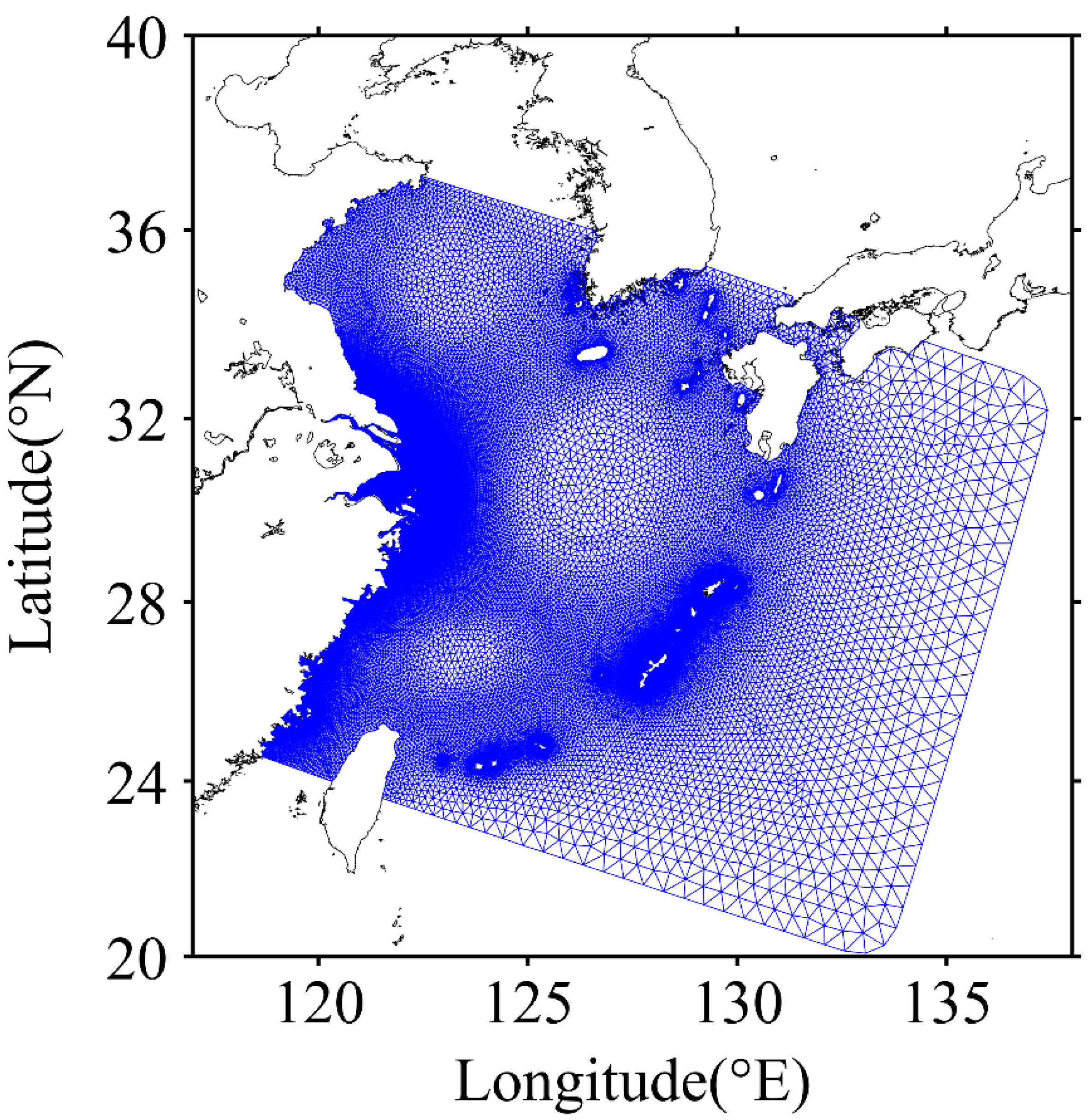
2.1. Study Area
2.2. Model Description
2.3. Diagnostic Typhoon Model
2.4. Extreme Value Analysis
3. Model Assessment
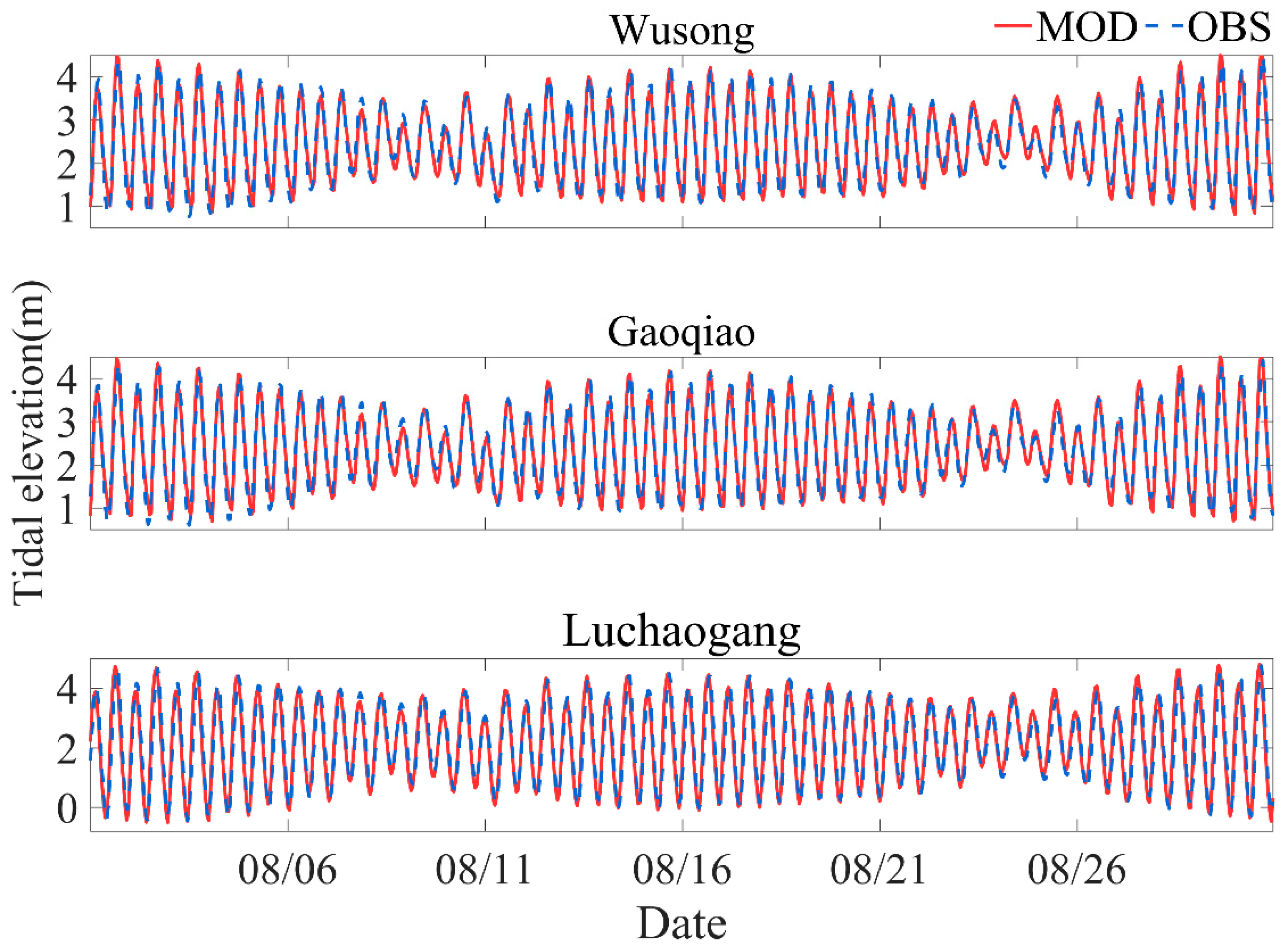
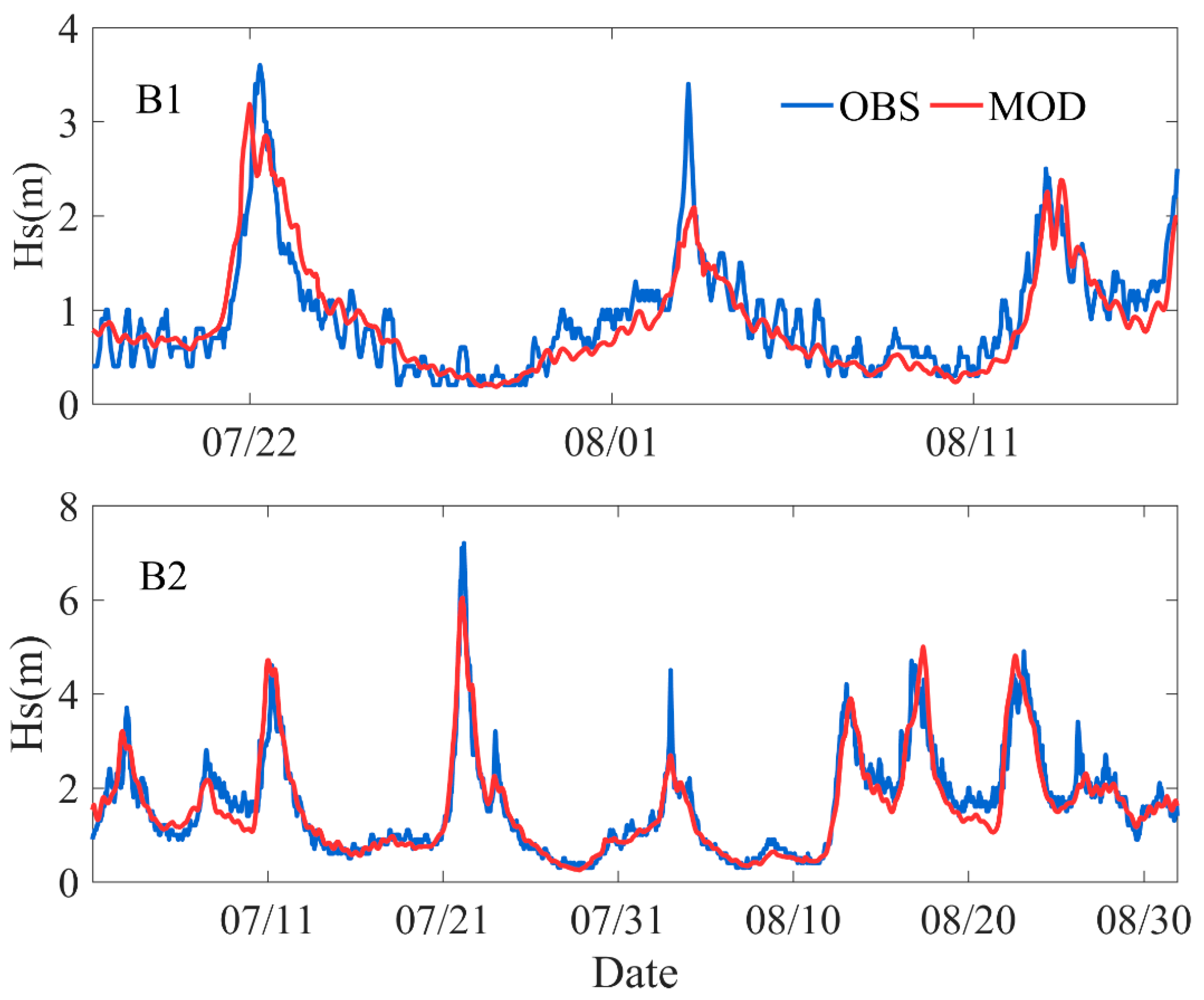
3.1. Tide and Wave Validation
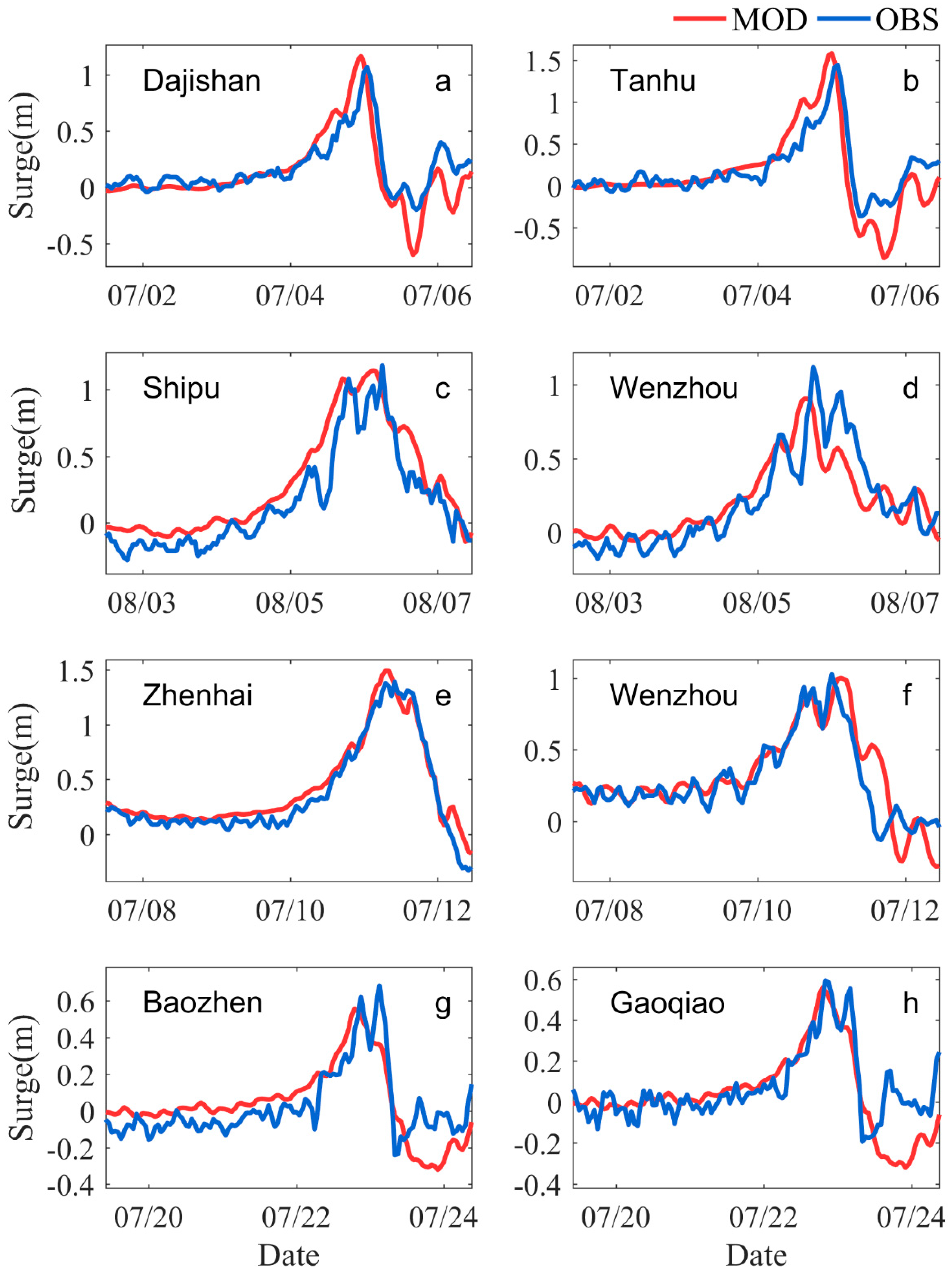
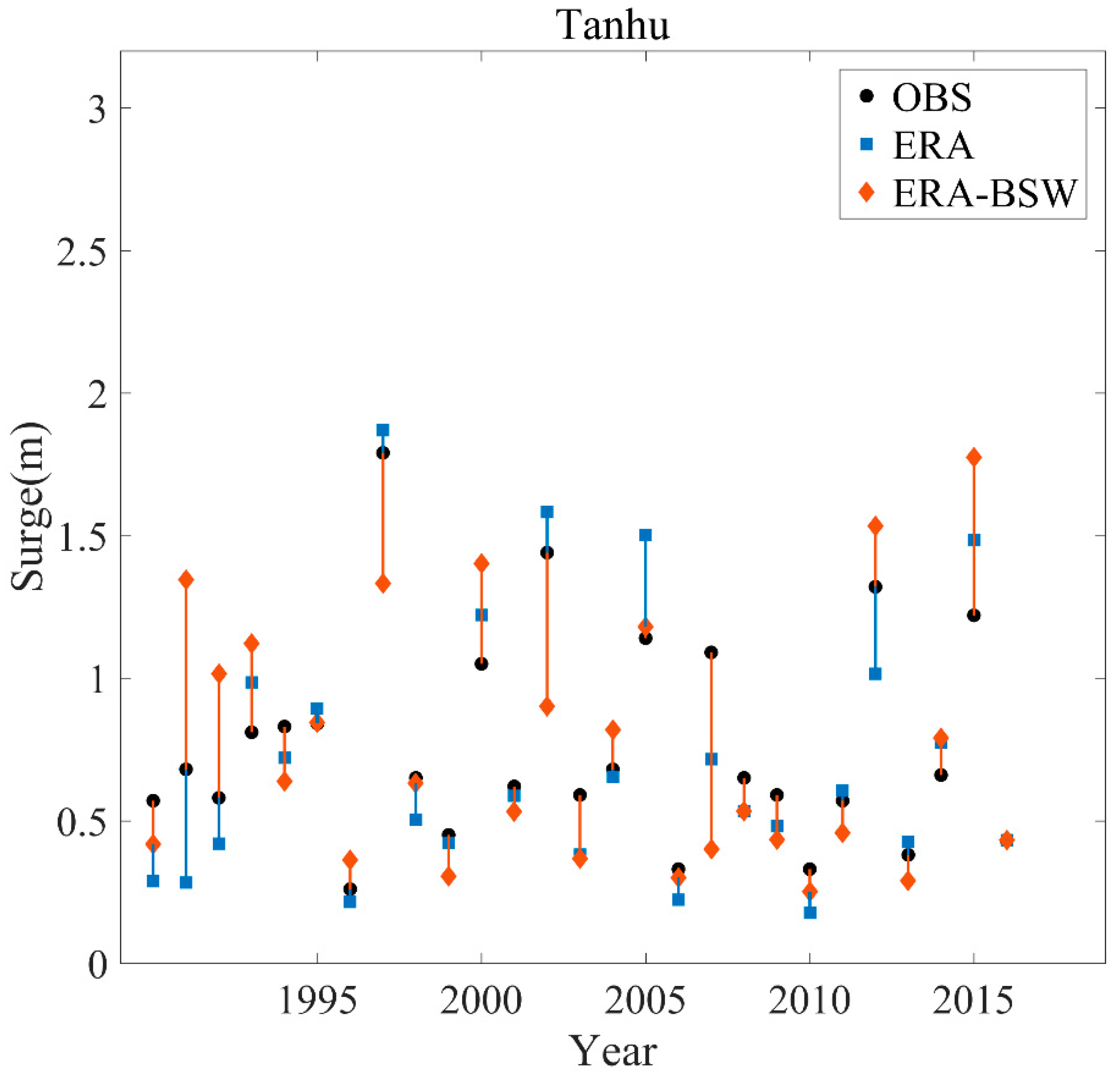
3.2. Storm Surges Validation
4. Result
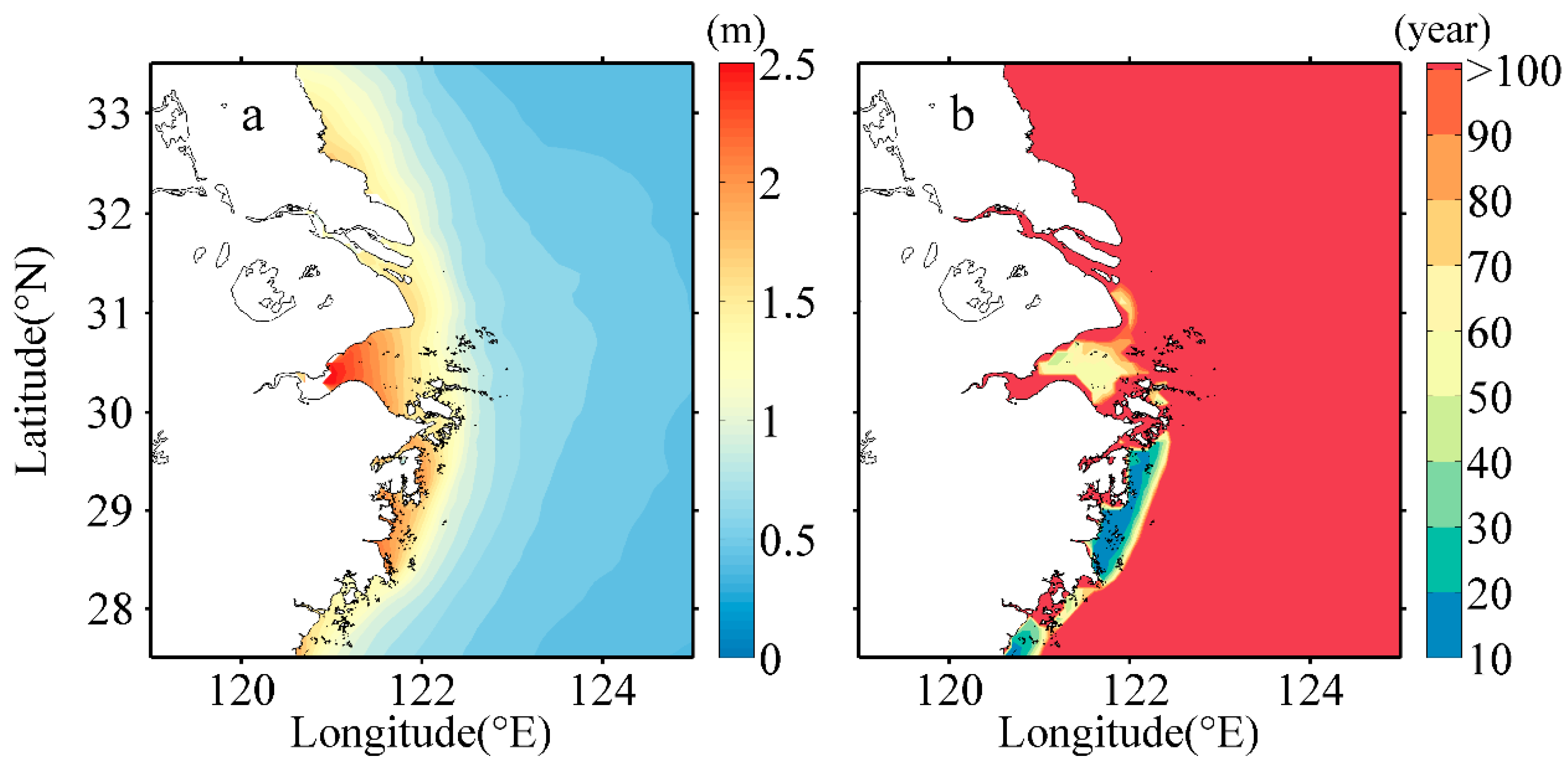
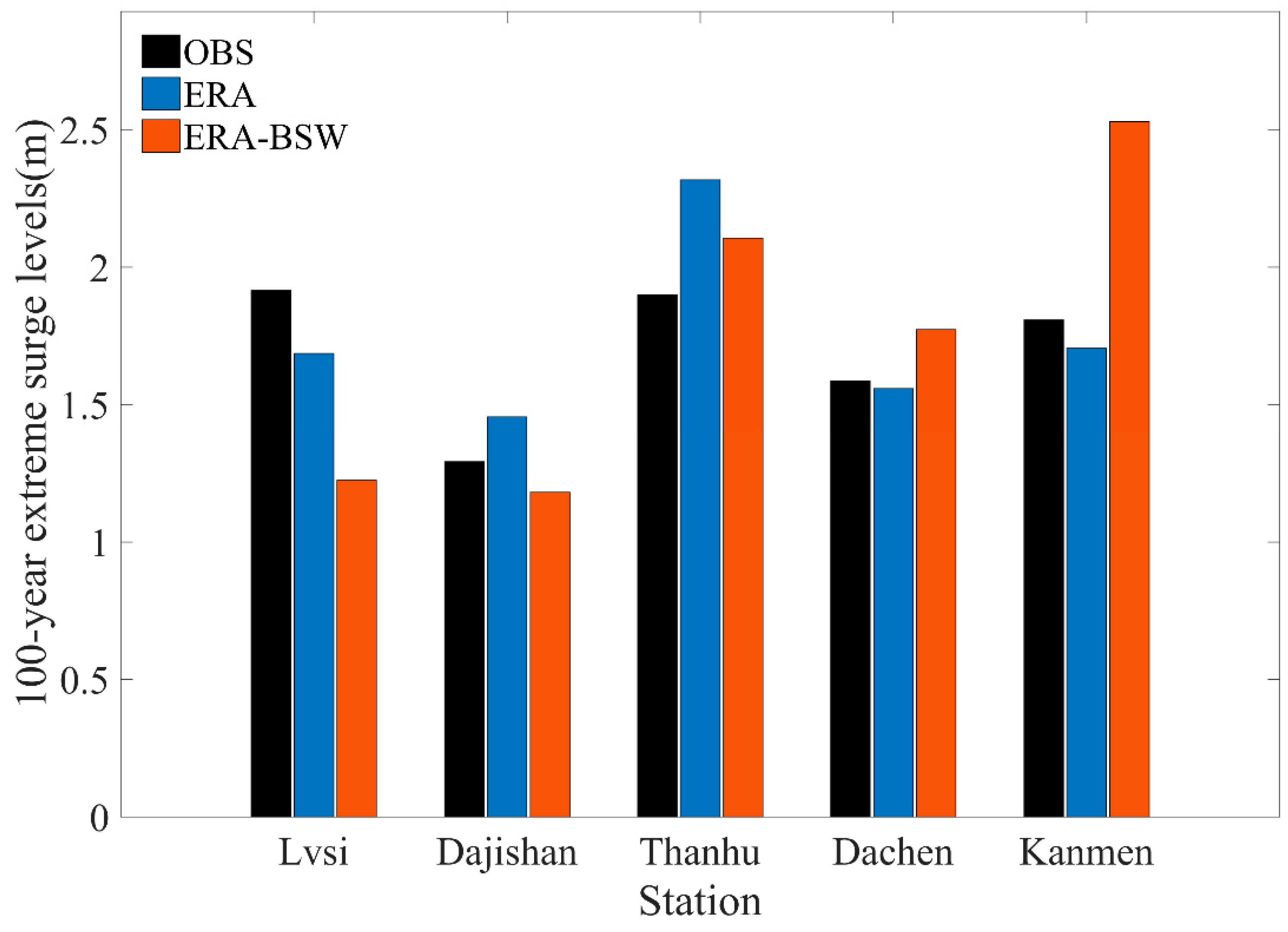
4.1. Extreme Surge Levels
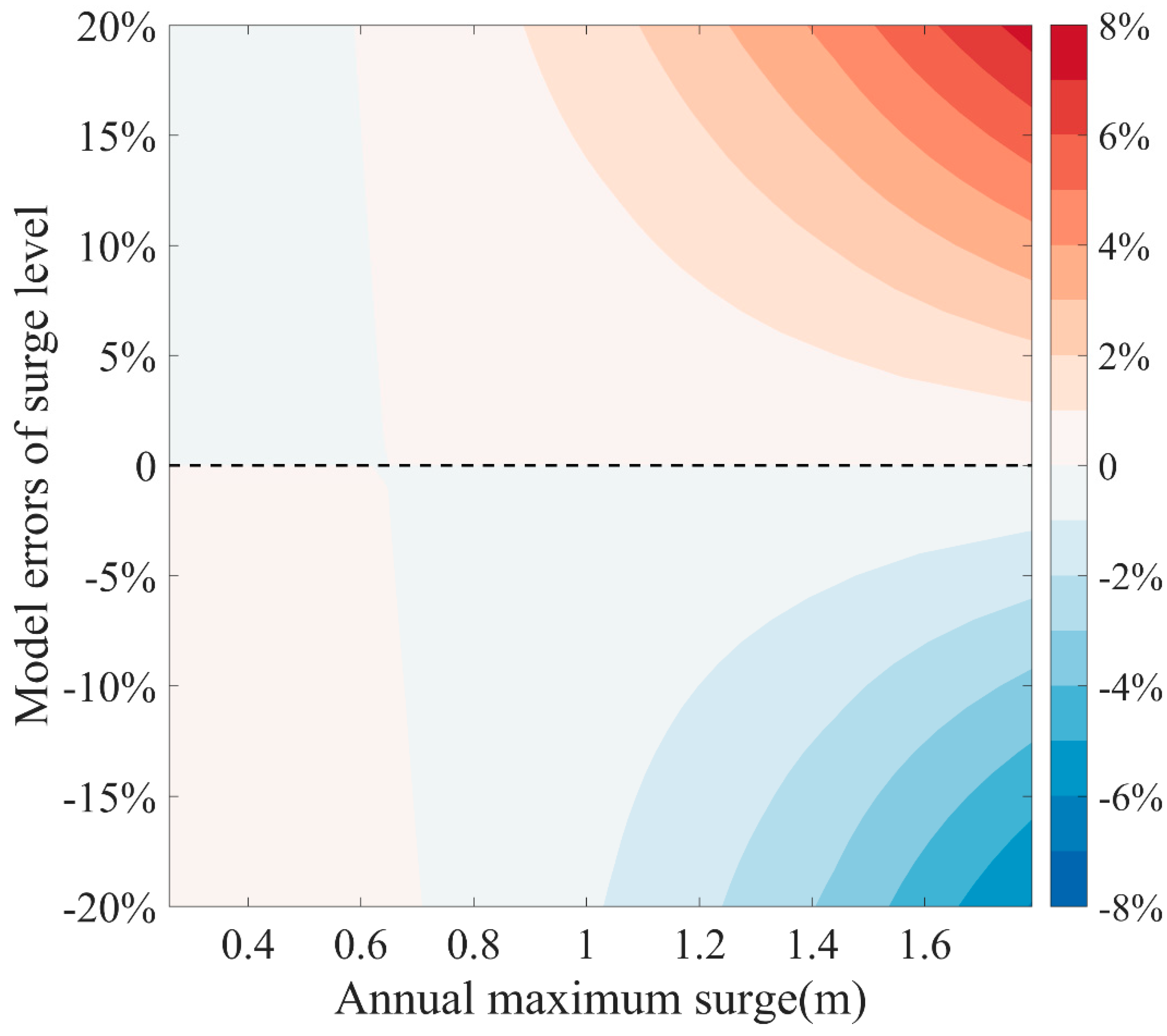
4.2. Wave Effects on Evaluation of Extreme Surge Levels
4.3. Joint Probability Analysis of Extreme Wave Heights and Surges
5. Discussion
6. Conclusions
Author Contributions
Funding
Institutional Review Board Statement
Informed Consent Statement
Data Availability Statement
Acknowledgments
Conflicts of Interest
References
- Xu, D.; Shu, A.; Shen, F. Effects of Clear-Sky Assimilation of GPM Microwave Imager on the Analysis and Forecast of Typhoon “Chan-Hom”. Sensors 2020, 20, 2674. [Google Scholar] [CrossRef]
- Chen, H.; Hua, F.; Yuan, Y. Seasonal characteristics and temporal variations of ocean wave in the Chinese offshore waters and adjacent sea areas. Adv. Mar. Sci. 2006, 24, 407–415. (In Chinese) [Google Scholar]
- Muis, S.; Apecechea, M.I.; Dullaart, J.; Lima, R.J.; Madsen, K.S.; Su, J.; Yan, K.; Verlaan, M. A high-resolution global dataset of extreme sea levels, tides, and storm surges, including future projections. Front. Mar. Sci. 2020, 7, 263. [Google Scholar] [CrossRef]
- Bloemendaal, N.; Muis, S.; Haarsma, R.J.; Verlaan, M.; Apecechea, M.I.; de Moel, H.; Ward, P.J.; Aerts, J.C. Global modeling of tropical cyclone storm surges using high-resolution forecasts. Clim. Dyn. 2019, 52, 5031–5044. [Google Scholar] [CrossRef] [Green Version]
- Zhang, H.; Sheng, J. Examination of extreme sea levels due to storm surges and tides over the northwest Pacific Ocean. Cont. Shelf Res. 2015, 93, 81–97. [Google Scholar] [CrossRef]
- Pan, Z.-h.; Liu, H. Extreme storm surge induced coastal inundation in Yangtze Estuary regions. J. Hydrodyn. 2019, 31, 1127–1138. [Google Scholar] [CrossRef]
- Sahoo, B.; Bhaskaran, P.K. A comprehensive data set for tropical cyclone storm surge-induced inundation for the east coast of India. Int. J. Climatol. 2018, 38, 403–419. [Google Scholar] [CrossRef]
- Sahoo, B.; Sahoo, T.; Bhaskaran, P.K. Wave–current-surge interaction in a changing climate over a shallow continental shelf region. Reg. Stud. Mar. Sci. 2021, 46, 101910. [Google Scholar]
- Gayathri, R.; Murty, P.; Bhaskaran, P.K.; Kumar, T.S. A numerical study of hypothetical storm surge and coastal inundation for AILA cyclone in the Bay of Bengal. Environ. Fluid Mech. 2016, 16, 429–452. [Google Scholar]
- Bhaskaran, P.K.; Gayathri, R.; Murty, P.; Bonthu, S.; Sen, D. A numerical study of coastal inundation and its validation for Thane cyclone in the Bay of Bengal. Coast. Eng. 2014, 83, 108–118. [Google Scholar] [CrossRef]
- Murty, P.; Sandhya, K.; Bhaskaran, P.K.; Jose, F.; Gayathri, R.; Nair, T.B.; Kumar, T.S.; Shenoi, S. A coupled hydrodynamic modeling system for PHAILIN cyclone in the Bay of Bengal. Coast. Eng. 2014, 93, 71–81. [Google Scholar] [CrossRef]
- Murty, P.; Bhaskaran, P.K.; Gayathri, R.; Sahoo, B.; Kumar, T.S.; SubbaReddy, B. Numerical study of coastal hydrodynamics using a coupled model for Hudhud cyclone in the Bay of Bengal. Estuar. Coast. Shelf Sci. 2016, 183, 13–27. [Google Scholar] [CrossRef]
- Poulose, J.; Rao, A.; Bhaskaran, P.K. Role of continental shelf on non-linear interaction of storm surges, tides and wind waves: An idealized study representing the west coast of India. Estuar. Coast. Shelf Sci. 2018, 207, 457–470. [Google Scholar]
- Wang, K.; Hou, Y.; Li, S.; Du, M.; Lu, J. A comparative study of storm surge and wave setup in the East China Sea between two severe weather events. Estuar. Coast. Shelf Sci. 2020, 235, 106583. [Google Scholar] [CrossRef]
- Kuang, C.; Chen, K.; Wang, J.; Wu, Y.; Liu, X.; Xia, Z. Responses of Hydrodynamics and Saline Water Intrusion to Typhoon Fongwong in the North Branch of the Yangtze River Estuary. Appl. Sci. 2021, 11, 8986. [Google Scholar] [CrossRef]
- Funakoshi, Y.; Hagen, S.C.; Bacopoulos, P. Coupling of Hydrodynamic and Wave Models: Case Study for Hurricane Floyd (1999) Hindcast. J. Waterw. Port Coast. Ocean Eng. 2008, 134, 321–335. [Google Scholar]
- Xie, D.M.; Zou, Q.P.; Cannon, J.W. Application of SWAN+ADCIRC to tide-surge and wave simulation in Gulf of Maine during Patriot’s Day storm. Water Sci. Eng. 2016, 9, 33–41. [Google Scholar] [CrossRef] [Green Version]
- Yu, X.; Pan, W.; Zheng, X.; Zhou, S.; Tao, X. Effects of wave-current interaction on storm surge in the Taiwan Strait: Insights from Typhoon Morakot. Cont. Shelf Res. 2017, 146, 47–57. [Google Scholar] [CrossRef]
- Hu, K.; Ding, P.; Ge, J. Modelling of Storm Surge in the Coastal Waters of Yangtze Estuary and Hangzhou Bay, China. J. Coast. Res. 2007, 50, 527–533. [Google Scholar]
- Guo, Y.; Zhang, J.; Zhang, L.; Shen, Y. Computational investigation of typhoon-induced storm surge in Hangzhou Bay, China. Estuar. Coast. Shelf Sci. 2009, 85, 530–536. [Google Scholar] [CrossRef]
- Pan, Z.; Liu, H. Impact of human projects on storm surge in the Yangtze Estuary. Ocean Eng. 2020, 196, 106792. [Google Scholar] [CrossRef]
- Haselsteiner, A.F.; Thoben, K.D. Predicting wave heights for marine design by prioritizing extreme events in a global model. Renew. Energy 2020, 156, 1146–1157. [Google Scholar] [CrossRef]
- Dong, S.; Gao, J.; Xue, L.I.; Wei, Y.; Wang, L. A Storm Surge Intensity Classification Based on Extreme Water Level and Concomitant Wave Height. J. Ocean Univ. China 2015, 14, 237–244. [Google Scholar] [CrossRef]
- Feng, J.; Jiang, W. Extreme water level analysis at three stations on the coast of the Northwestern Pacific Ocean. Ocean Dyn. 2015, 65, 1383–1397. [Google Scholar] [CrossRef]
- Mazas, F.; Hamm, L. An event-based approach for extreme joint probabilities of waves and sea levels. Coast. Eng. 2017, 122, 44–59. [Google Scholar] [CrossRef]
- Bruun, J.T.; Tawn, J.A. Comparison of approaches for estimating the probability of coastal flooding. J. R. Stat. Soc. Ser. C 1998, 47, 405–423. [Google Scholar] [CrossRef]
- Resio, D.T.; Irish, J.; Cialone, M. A surge response function approach to coastal hazard assessment—Part 1: Basic concepts. Nat. Hazards 2009, 51, 163–182. [Google Scholar] [CrossRef]
- Toro, G.R.; Resio, D.T.; Divoky, D.; Niedoroda, A.W.; Reed, C. Efficient joint-probability methods for hurricane surge frequency analysis. Ocean Eng. 2010, 37, 125–134. [Google Scholar] [CrossRef]
- Yin, K.; Xu, S.; Huang, W. Estimating extreme sea levels in Yangtze Estuary by quadrature Joint Probability Optimal Sampling Method. Coast. Eng. 2018, 140, 331–341. [Google Scholar] [CrossRef]
- Wang, Y.; Mao, X.; Jiang, W. Long-term hazard analysis of destructive storm surges using the ADCIRC- SWAN model: A case study of Bohai Sea, China. Int. J. Appl. Earth Obs. Geoinf. 2018, 73, 52–62. [Google Scholar]
- Li, J.; Pan, S.; Chen, Y.; Fan, Y.M.; Pan, Y. Numerical estimation of extreme waves and surges over the northwest Pacific Ocean. Ocean Eng. 2018, 153, 225–241. [Google Scholar]
- Chen, Y.; Li, J.; Pan, S.; Gan, M.; Pan, Y.; Xie, D.; Clee, S. Joint probability analysis of extreme wave heights and surges along China’s coasts. Ocean Eng. 2019, 177, 97–107. [Google Scholar] [CrossRef]
- Yoon, J.-J.; Jun, K.-C. Coupled storm surge and wave simulations for the Southern Coast of Korea. Ocean Sci. J. 2015, 50, 9–28. [Google Scholar] [CrossRef]
- Rong, Z.; Li, M. Tidal effects on the bulge region of Changjiang River plume. Estuar. Coast. Shelf Sci. 2012, 97, 149–160. [Google Scholar]
- Yuan, R.; Wu, H.; Zhu, J.; Li, L. The response time of the Changjiang plume to river discharge in summer. J. Mar. Syst. 2016, 154, 82–92. [Google Scholar]
- Luan, H.L.; Ding, P.X.; Wang, Z.B.; Ge, J.Z.; Yang, S.L. Decadal morphological evolution of the Yangtze Estuary in response to river input changes and estuarine engineering projects. Geomorphology 2016, 265, 12–23. [Google Scholar] [CrossRef]
- Guo, L.; van der Wegen, M.; Jay, D.A.; Matte, P.; Wang, Z.B.; Roelvink, D.; He, Q. River-tide dynamics: Exploration of nonstationary and nonlinear tidal behavior in the Y angtze R iver estuary. J. Geophys. Res. Ocean. 2015, 120, 3499–3521. [Google Scholar] [CrossRef] [Green Version]
- Jiang, X.; Guan, C.; Wang, D. Rogue waves during Typhoon Trami in the East China Sea. J. Oceanol. Limnol. 2019, 37, 1817–1836. [Google Scholar] [CrossRef]
- Zhang, M.; Townend, I.; Cai, H.; He, J.; Mei, X. The influence of seasonal climate on the morphology of the mouth-bar in the Yangtze Estuary, China. Cont. Shelf Res. 2018, 153, 30–49. [Google Scholar] [CrossRef] [Green Version]
- Ding, Y.H.; Chan, J.C. The East Asian summer monsoon: An overview. Meteorol. Atmos. Phys. 2005, 89, 117–142. [Google Scholar]
- Wu, Y.; Bao, H.; Yu, H.; Zhang, J.; Kattner, G. Temporal variability of particulate organic carbon in the lower Changjiang (Yangtze River) in the post-Three Gorges Dam period: Links to anthropogenic and climate impacts. J. Geophys. Res. Biogeosci. 2015, 120, 2194–2211. [Google Scholar] [CrossRef] [Green Version]
- Ke, Q.; Jonkman, S.N.; Van Gelder, P.H.; Bricker, J.D. Frequency Analysis of Storm-Surge-Induced Flooding for the Huangpu River in Shanghai, China. J. Mar. Sci. Eng. 2018, 6, 70. [Google Scholar] [CrossRef] [Green Version]
- Luettich, R.A.; Westerink, J.J. Formulation and NumericalIimplementation of the 2D/3D ADCIRC Finite Element Model Version 44.XX; University of North Carolina at Chapel Hill: Morehead City, NC, USA, 2004. [Google Scholar]
- Westerink, J.J.; Luettich, R.A.; Baptists, A.; Scheffner, N.W.; Farrar, P. Tide and storm surge predictions using finite element model. J. Hydraul. Eng. 1992, 118, 1373–1390. [Google Scholar]
- Demissie, H.K.; Bacopoulos, P. Parameter estimation of anisotropic Manning’s n coefficient for advanced circulation (ADCIRC) modeling of estuarine river currents (lower St. Johns River). J. Mar. Syst. 2017, 169, 1–10. [Google Scholar] [CrossRef]
- Booij, N.; Ris, R.C.; Holthuijsen, L.H. A third-generation wave model for coastal regions 1. Model description and validation. J. Geophys. Res. Atmos. 1999, 104, 7649–7666. [Google Scholar] [CrossRef] [Green Version]
- Dietrich, J.C.; Zijlema, M.; Westerink, J.J.; Holthuijsen, L.H.; Dawson, C.; Luettich, R.A.; Jensen, R.E.; Smith, J.M.; Stelling, G.S.; Stone, G.W. Modeling hurricane waves and storm surge using integrally-coupled, scalable computations. Coast. Eng. 2011, 58, 45–65. [Google Scholar]
- Yin, J.; Lin, N.; Yang, Y.; Pringle, W.J.; Tan, J.; Westerink, J.J.; Yu, D. Hazard Assessment for Typhoon-Induced Coastal Flooding and Inundation in Shanghai, China. J. Geophys. Res. Ocean. 2021, 126, e2021JC017319. [Google Scholar] [CrossRef]
- Nayak, S.; Bhaskaran, P.K.; Venkatesan, R. Near-shore wave induced setup along Kalpakkam coast during an extreme cyclone event in the Bay of Bengal. Ocean Eng. 2012, 55, 52–61. [Google Scholar]
- Egbert, G.D.; Erofeeva, S.Y. Efficient Inverse Modeling of Barotropic Ocean Tides. J. Atmos. Ocean. Technol. 2002, 19, 183–204. [Google Scholar] [CrossRef] [Green Version]
- Komen, G.; Hasselmann, S.; Hasselmann, K. On the existence of a fully developed wind-sea spectrum. J. Phys. Oceanogr. 1984, 14, 1271–1285. [Google Scholar] [CrossRef]
- Jelesnianski, C.P. A numerical calculation of storm tides induced by a tropical storm impinging on a continental shelf. Mon. Weather Rev. 1965, 93, 343–358. [Google Scholar] [CrossRef] [Green Version]
- Jelesnianski, C.P. SLOSH: Sea, Lake, and Overland Surges from Hurricanes; US Department of Commerce, National Oceanic and Atmospheric Administration: Washington, DC, USA, 1992; Volume 48.
- Dong, S.; Hao, X.L.; Fan, D.Q. Joint probability distribution of wind velocity and wave height in ocean engineering design. Acta Oceanol. Sin. 2005, 27, 85–89. (In Chinese) [Google Scholar]
- JMA. Operational Tropical Cyclone Analysis by the Japan Meteorological Agency. In Proceedings of the International Workshop on Satellite Analysis of Tropical Cyclones, Honolulu, HI, USA, 13–16 April 2011. [Google Scholar]
- Atkinson, G.D.; Holliday, C.R. Tropical Cyclone Minimum Sea Level Pressure-Maximum Sustained Wind Relationship for Western North Pacific. Mon. Weather Rev. 1977, 105, 421–427. [Google Scholar] [CrossRef] [Green Version]
- Willoughby, H.E.; Rahn, M.E. Parametric Representation of the Primary Hurricane Vortex. Part I: Observations and Evaluation of the Holland (1980) Model. Mon. Weather Rev. 2004, 134, 1102–1120. [Google Scholar] [CrossRef] [Green Version]
- Murty, P.; Srinivas, K.S.; Rao, E.P.R.; Bhaskaran, P.K.; Shenoi, S.; Padmanabham, J. Improved cyclonic wind fields over the Bay of Bengal and their application in storm surge and wave computations. Appl. Ocean Res. 2020, 95, 102048. [Google Scholar] [CrossRef]
- Zhang, J.; Xiong, M.; Yin, C.; Gan, S. Inner shelf response to storm track variations over the east LeiZhou Peninsula, China. Int. J. Appl. Earth Obs. Geoinf. 2018, 71, 56–69. [Google Scholar]
- Liu, D.; Pang, L.; Xie, B.; Wu, Y. Study of typhoon disaster zoning in China: Double layer nested multi-objective probability model. Sci. China 2008, 38, 698–707. (In Chinese) [Google Scholar]
- Yang, X.C.; Zhang, Q.H. Joint probability distribution of winds and waves from wave simulation of 20 years (1989–2008) in Bohai Bay. Water Sci. Eng. 2013, 3, 296–307. [Google Scholar]
- Pinheiro, E.C.; Ferrari, S. A comparative review of generalizations of the extreme value distribution. J. Stat. Comput. Simul. 2015, 86, 2241–2261. [Google Scholar] [CrossRef] [Green Version]
- Castillo, E. Extreme Value Theory in Engineering; Academic Press: New York, NY, USA, 1988. [Google Scholar]
- Yue, S. The Gumbel logistic model for representing a multivariate storm event. Adv. Water Resour. 2000, 24, 179–185. [Google Scholar] [CrossRef]
- Tawn, J.A. Bivariate extreme value theory: Models and estimation. Biometrika 1988, 75, 397–415. [Google Scholar] [CrossRef]
- Wang, N.; Hou, Y.; Mo, D.; Li, J. Hazard assessment of storm surges and concomitant waves in Shandong Peninsula based on long-term numerical simulations. Ocean Coast. Manag. 2021, 213, 105888. [Google Scholar] [CrossRef]
- Li, M.; Zhong, L. Tidal energy fluxes and dissipation in the Chesapeake Bay. Cont. Shelf Res. 2006, 26, 752–770. [Google Scholar]
- Fang, G.; Wang, Y.; Wei, Z.; Choi, B.H.; Wang, X.; Wang, J. Empirical cotidal charts of the Bohai, Yellow, and East China Seas from 10 years of TOPEX/Poseidon altimetry. J. Geophys. Res. Ocean. 2004, 109, C11006. [Google Scholar] [CrossRef]
- Yin, C.; Zhang, W.; Xiong, M.; Wang, J.; Zhang, J. Storm surge responses to the representative tracks and storm timing in the Yangtze Estuary, China. Ocean Eng. 2021, 233, 109020. [Google Scholar]
- Lai, F.; Liu, L.; Liu, H. Wave Effects on the Storm Surge Simulation: A Case Study of Typhoon Khanun. J. Disaster Res. 2016, 11, 964–972. [Google Scholar] [CrossRef]
- Li, A.; Guan, S.; Mo, D.; Hou, Y.; Liu, Z. Modeling wave effects on storm surge from different typhoon intensities and sizes in the South China Sea. Estuar. Coast. Shelf Sci. 2019, 235, 106551. [Google Scholar] [CrossRef]
- Li, S.; Sha, W.; Qi, Y. Joint Probability Analysis of Numerical Simulation Results of Typhoon Wave and Storm Surge of the Wulei Station at the Beibu Bay. Mar. Sci. Bull. 2006, 25, 23–28. [Google Scholar]
- Kim, S.; Anh, T.N.; Nguyen, K.C.; Thc, P.T.; Thuy, N.B. The influence of moving speeds, wind speeds, and sea level pressures on after- runner storm surges in the Gulf of Tonkin, Vietnam. Ocean Eng. 2020, 212, 107613. [Google Scholar]


| Station | ERA | ERA-BSW |
|---|---|---|
| LVSI | −14.82% | −18.17% |
| DAJISHAN | −3.92% | −10.86% |
| TANHU | 1.52% | −0.65% |
| DACHEN | −13.60% | 4.73% |
| KANMEN | −1.61% | 12.52% |
Publisher’s Note: MDPI stays neutral with regard to jurisdictional claims in published maps and institutional affiliations. |
© 2021 by the authors. Licensee MDPI, Basel, Switzerland. This article is an open access article distributed under the terms and conditions of the Creative Commons Attribution (CC BY) license (https://creativecommons.org/licenses/by/4.0/).
Share and Cite
Chi, Y.; Rong, Z. Assessment of Extreme Storm Surges over the Changjiang River Estuary from a Wave-Current Coupled Model. J. Mar. Sci. Eng. 2021, 9, 1222. https://doi.org/10.3390/jmse9111222
Chi Y, Rong Z. Assessment of Extreme Storm Surges over the Changjiang River Estuary from a Wave-Current Coupled Model. Journal of Marine Science and Engineering. 2021; 9(11):1222. https://doi.org/10.3390/jmse9111222
Chicago/Turabian StyleChi, Yutao, and Zengrui Rong. 2021. "Assessment of Extreme Storm Surges over the Changjiang River Estuary from a Wave-Current Coupled Model" Journal of Marine Science and Engineering 9, no. 11: 1222. https://doi.org/10.3390/jmse9111222
APA StyleChi, Y., & Rong, Z. (2021). Assessment of Extreme Storm Surges over the Changjiang River Estuary from a Wave-Current Coupled Model. Journal of Marine Science and Engineering, 9(11), 1222. https://doi.org/10.3390/jmse9111222