A Study on the Effectiveness of the Heading Control on the Mooring Line Tension and Position Offset for an Arctic Floating Structure under Complex Environmental Loads

Abstract

Even though interest in developing the Arctic region is increasing continuously, the standard procedure to be used to analyze the station-keeping performance of a floater considering ice loads has not been established yet. In this paper, the effectiveness of heading control with a dynamic positioning system is analyzed to evaluate the improvement of the performance of the station-keeping system in the ice conditions. Complex environmental loads with ice-induced forces were generated and applied to a ship type floater with dynamic positioning and mooring systems. Three-hour time-domain simulations were conducted for the two different station-keeping systems with mooring only and mooring with a dynamic positioning system. Position offsets and mooring line tensions for the two scenarios were compared with maximum values and most probable maxima (MPM) values. The results of the simulation showed that the heading control can reduce 8.2% of MPM values for the mooring lines and improve the station-keeping performance by about 16.3%. The validity of the station-keeping system that was designed was confirmed, and it is expected that the specification of mooring lines can be relaxed with the heading control.

1. Introduction

Floating offshore structures must have station-keeping capability to conduct the requested work in stable conditions. The position of a floating-type production platform is required to be within 10% of the installed water depth for the safety of risers. Generally, mooring systems and dynamic positioning (DP) systems are used for the station-keeping of floating structures. Two types of mooring systems have been used extensively, i.e., spread mooring and single point mooring with turret. Turret systems commonly are installed in severe environments. In the Arctic region, the ice induced load must be considered in designing a station-keeping system.

One of the most serious problems for a turret system in ice conditions is the difficulty in weathervaning, which is the main advantage of the system. The turret makes the floater align with the direction of the significant environmental load. However, when the attack angle of the ice field is over a certain range, the restoration force is not enough to rotate, and the floater begins to drift in the direction that the ice field is moving. This results in excessive tension on the mooring lines, and they may break [1].

To prevent this situation, either a DP assisted mooring (DPAM) system or a thruster-assisted mooring (TAM) system can be used. DPAM has been used in severe environments for station-keeping purposes. Ice conditions are one such environment, and DPAM can be considered as a solution. Thrusters can give enough moment to turn the floating structure to the direction of the wind or the directions of other significant forces. This leads to the reduction of the tension in the mooring lines.

In designing DPAM, the designs of the mooring line and the DP system are considered at the same time. There are two main approaches in designing a mooring system, i.e., the static frequency-domain approach and the dynamic time-domain approach. The frequency-domain analysis has advantages in time and the possible combination of various environmental conditions. These characteristics are useful in the initial basic design stage. However, due to the limitation of the accuracy of nonlinear coupled analysis, the time-domain analysis also must be conducted [2]. After the analyses of the equilibrium position analysis and the linear frequency response, variations in the tension of the mooring lines are monitored in a time-domain analysis. The results are used to predict the fatigue damage during the design life and to decide the final arrangement of the mooring line [3]. The performance of DPAM in the time domain can be evaluated by observing the offset of the position and monitoring the variation in the tension of the mooring line. The location of the floater must be within the allowable radius, and the statistically processed tensions on the designed mooring lines must be less than 60% of the maximum breaking load (MBL) [4]. The previous research on the station-keeping of a floater in the Arctic region is inadequate for considering complex environmental loads that include ice forces as well as the loads associated with the wind, waves, and currents.

In the time domain, the station-keeping performance considers the operational and survival conditions in which the designed structure will be operated. The wind, current, and wave conditions are defined well in the many rules and standards of the classification societies. However, to date, evaluation methods and design standards that consider the ice load have not been provided. The most difficult thing in considering the ice load is to assess the effect of the load on the station-keeping performance.

There are three major methods that are used to evaluate the station-keeping performance in ice-covered waters, i.e., on-site operations, ice tank tests, and computer simulations. In 2004, the International Ocean Drilling Program (IODP) conducted 302 arctic coring expedition, and collected data concerning the difficulties associated with maintaining a given position in the ice [5,6,7]. As a part of the project entitled dynamic positioning in ice condition, i.e., the DYPIC project, a model test was conducted for an Arctic drilling vessel in 2014 [8,9]. In addition, Canada’s National Research Council (NRC) also conducted an ice tank test for a drilling vessel [10]. However, these on-site tests and ice tank tests are expensive and have limitations when it comes to changing the test conditions.

To overcome these limitations, there are active research programs related to the simulation of ice–structure interactions. The numerical methods generally use the discrete element method (DEM), and simulations are being conducted on station-keeping in ice conditions, ice-structure interactions, and the navigation of ships in ice-covered waters [11,12,13]. To reduce the time required for the simulations, researchers used the graphical processing unit (GPU) to develop the GPU event mechanics (GEM) for use in acquiring a good floating-point calculation [14,15]. Such software still has limitations, i.e., the direction in which the ice is drifting cannot be changed, and other environmental loads, such as the wave load, have not been incorporated in the program.

Recently, ice load generation methods that consist of complex environmental loads have been suggested for the evaluation of station-keeping performance in the time domain. In [16], an ice load generation method was proposed by combining the mean values of the ice load from the ice tank test and the spectrum values from GEM. Another similar method that generates ice forces on the structure at an arbitrary heading angle was introduced for use in the time-domain analysis [17].

This paper is focused on the evaluation of the station-keeping performance of a floating production structure using the ice load generation module. The DP system is added for the heading control to the mooring system, and simulations are conducted to appraise the effectiveness of the DP system. A complex environmental condition was set by considering the target site. Then, time-domain simulations are conducted for two scenarios, i.e., mooring only and DPAM. The results are processed, and the effectiveness of the DPAM is examined over the mooring system. The rest of the paper is organized as follows.

The fundamentals in analyzing the performance of the station-keeping are summarized in Section 2. The third section describes the information about the target floater, the ice load generation module, and settings for the time-domain simulation. The results are reviewed in Section 4. The variations of the position offset and mooring tension are observed, and the performance was evaluated using the most probable maxima values. The results are summarized in Section 5, and the advantage of the heading control is described. Additionally, the limitations of the research and future works are discussed.

2. Dynamics in Ice Condition and Procedure to Evaluate the Station-Keeping Performance

2.1. Frequency-Domain Analysis

An analysis of the motion of an offshore floater is to get a solution of the Laplace equation, which is composed of velocity potentials. The pressure acting on the surface of the floater in a fluid field is derived from the following Equation (1):

$$P_{Fluid}=-\rho gz-\rho \frac{\partial \Phi }{\partial t}=-\rho gz-\rho \left(\frac{\partial {\Phi }_I}{\partial t}+\frac{\partial {\Phi }_D}{\partial t}+\frac{\partial {\Phi }_R}{\partial t}\right)=P_{Static}+P_{F.K.}+P_D+P_R,$$

(1)

where $\rho$ is the density of water, $g$ is the gravitational acceleration, $z$ is the depth, and $t$ is the time. ${\Phi }_I,{\Phi }_D,{\Phi }_R$ are the incident, diffraction, and radiation potentials, respectively. In the rightmost term, $P_{Static}$ is the static pressure, $P_{F.K.}$ is the Froude–Krylrov pressure, $P_D$ is the diffraction pressure, and $P_R$ is the radiation pressure. By integrating the pressure for the entire submerged area of the floater, the pressure terms in Equation (1) can be converted to forces and expressed as Equation (2) by Newton’s law of motion.

$$M\ddot{x}=F_{Gravity}+F_{static}+F_{F.K.}+F_D+F_R$$

(2)

After calculating hydrostatic and hydrodynamic coefficients with the incident angles and frequencies of the waves acting on the structure, the motion ratio amplitude operator (RAO) of the floater is computed in the frequency-domain analysis. The results are used to evaluate the motion characteristics of the floater designed to be operated at the target site.

2.2. Time-Domain Analysis

Since the floater was modeled and designed as a linear system, the characteristics of the nonlinear elements are not represented well in the frequency-domain analysis. To resolve these limitations, time-domain analysis is required [18]. Generally, the equation of motion for a floater can be expressed as shown in Equation (3) for the time-domain analysis.

$$M\ddot{x}=-Kx+F_{exciting}-A\ddot{x}-C\dot{x}+F_{External}$$

(3)

For a floater with mass M, $F_{Gravity}$ is the body force, and $F_{static}, F_{F.K},F_D,\mathrm{and}{F}_R$ are the surface forces by the fluid. $F_{Gravity}$ and $F_{static}$ compose the restoration force ($Kx$). $F_{F.K}$ and $F_D$ are wave excitation forces ($F_{exciting}$). The radiation force, $F_R$, is composed of mass and damping terms ($F_R=-A\ddot{x}-B\dot{x}$), where A is the added mass, and B is the damping coefficient. $F_{External}$ means all other environmental forces in the Arctic region, which include wind, current, and ice loads. After transpositioning the added mass term, the damping and restoration terms on the right side of Equation (3) can be expressed as shown in the following Equation (4):

$$\left(M+A\right)\ddot{x}+C\dot{x}+Kx=F_{exciting}+F_{wind}+F_{current}+F_{DP}+F_{mooring}+F_{ice}$$

(4)

where $F_{wind}$, $F_{current}$, and $F_{ice}$ denote the wind, current, and ice forces, respectively. $F_{DP}$ and $F_{mooring}$ are the forces by the station-keeping system with DP and mooring.

2.3. Forces by the Station Keeping System

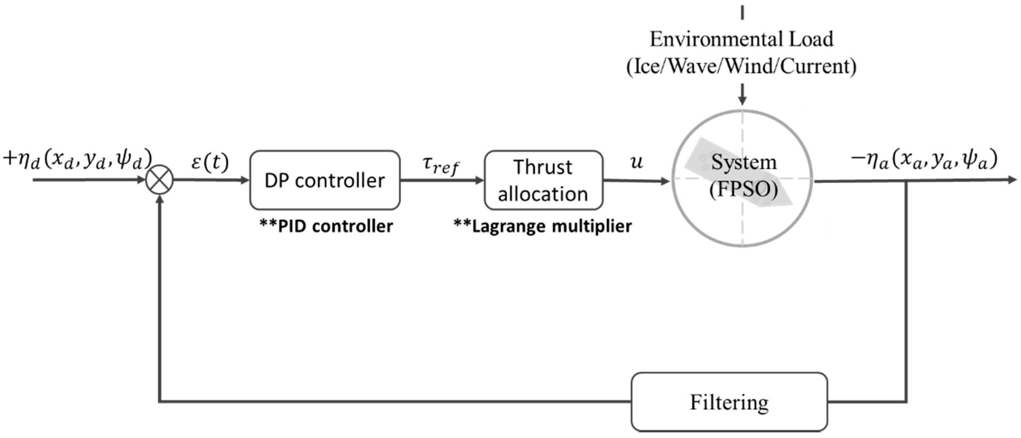
2.3.1. Force by the DP System

Generally, PID control logic is used for a DP system on a floating offshore structure. Figure 1 shows the general form of a DP control system. The logic uses the error and the rate of change of the error from the target state (${\eta }_d$) and the current state (${\eta }_a$). Considering the proportional gain ($K_P$), derivative gain ($K_d$), and integral gain ($K_i$), the required thrust can be derived from the following Equation (5):

$${\mathit{\tau }}_{ref}\left(t\right)=K_P\epsilon \left(t\right)+K_I{{\displaystyle \int }}_0^t\epsilon \left(\tau \right)d\tau +K_D\dot{\epsilon }\left(t\right)$$

(5)

$F_{x,ref}$, $F_{y,ref}$, and $M_{z,ref}$ are the forces required to restore the surge, sway, and yaw motion of the floater. Then, the required thrust can be summarized as shown in Equation (6):

$${\mathit{\tau }}_{ref}={\left[F_{x,ref},F_{y,ref},M_{z,ref}\right]}^T$$

(6)

For a DP system with n thrusters, the thrust vector for each propulsion system can be expressed as follows:

$${\mathit{u}}_i=\left(u_i{,}_x,u_i{,}_y\right),$$

(7)

where $u_{i,x}$ and $u_{i,y}$ are the forces of the ith propulsion system acting in the x-direction and y-direction in the body-fixed coordinate. The moment is calculated based on the center of gravity $\left(x_{CoG},y_{CoG}\right)$ and the locations of the thruster $\left(x_{CoG},y_{CoG}\right)$, i.e.,:

$$\begin{gathered} L_{i,x}=x_i-x_{CoG}, \\ {L}_{i,y}=y_i-y_{CoG}. \end{gathered}$$

(8)

Forces on the floater by $u_i$ can be summarized as:

$$\begin{gathered} F_{i,x}=u_{i,x}, \\ {F}_{i,y}=u_{i,y}, \\ {M}_{i,z}=L_{i,x}{u}_{i,y}-L_{i,y}{u}_{i,x}, \end{gathered}$$

(9)

which can be formularized as the following;

$$\left[\begin{array}{cc}1& 0\\ 0& 1\\ -L_{i,y}& L_{i,x}\end{array}\right]\left[\begin{array}{c}{u}_{i,x}\\ u_{i,y}\end{array}\right]=\left[\begin{array}{c}{F}_{i,x}\\ F_{i,y}\\ M_{i,z}\end{array}\right]\leftrightarrow B_i{\mathit{u}}_i=F_i$$

(10)

To keep the floater at the desired position, n thrusters are required to generate the required thrust, as shown in Equation (11):

$$B\mathit{u}={\mathit{\tau }}_{ref}$$

(11)

where

$$B=\left[B_1\dots B_i\dots B_n\right], u={\left[u_1\dots u_i\dots u_n\right]}^T$$

(12)

The Lagrange multiplier method is the most popular method for the allocation of the thrust for each propulsion system, and it can be stated as follows:

$$\underset{u}{\min }{u}^{T}Wu\mathrm{s}.\mathrm{t}.B\mathit{u}={\mathit{\tau }}_{ref}$$

(13)

where $W$ is the weight matrix ($W\in {ℝ}^{2n\times 2n},B\in {ℝ}^{3\times 2n}\mathrm{and}u\in {ℝ}^{2n}$). Using the Karush–Kuhn–Tucker (KKT) conditions provides the following optimal solution:

$$u=W^{-1}{B}^T{\left(B{W}^{-1}{B}^T\right)}^{-1}{\mathit{\tau }}_{ref}$$

(14)

2.3.2. Force by the Mooring Lines

For a motion analysis in the time domain, mooring lines are modeled with the lumped mass method or the Morison elements method. In this paper, the Morison elements method is used to consider the drag force. As shown in Figure 2a, a mooring line is assumed to be the combination of circular slender cylinders [19]. Figure 2b shows the hydrodynamic force ($\stackrel{\rightharpoonup }{F_h})$, inertial load ($\stackrel{\rightharpoonup }{W}$), and structural loads ($\overrightarrow{T}, \overrightarrow{V}, \overrightarrow{T})$ that are applied to each element (cylinder). $\nabla S_e$ and $D_e$ are the length and diameter of the cylinder, respectively. Each element has two nodes, i.e., one at the anchor side (first node) and one at the floater side (second node). At the first node, $\overrightarrow{T}$ is the tension vector, $\overrightarrow{M}$ is the bending moment vector, and $\overrightarrow{V}$ is the shear force vector. Then, the equation of motion for the circular cylinder can be expressed as:

$$\begin{gathered} \frac{\partial \overrightarrow{T}}{\partial s_e}+\frac{\partial \overrightarrow{V}}{\partial s_e}+\stackrel{\rightharpoonup }{W}+\stackrel{\rightharpoonup }{F_h}=m\frac{{\partial }^2\overrightarrow{R}}{\partial t^2} \\ \frac{\partial \overrightarrow{M}}{\partial s_e}+\frac{\partial \overrightarrow{R}}{\partial s_e}\times \overrightarrow{V}=-\overrightarrow{q} \end{gathered}$$

(15)

where $m$ is the mass per unit length, $\overrightarrow{q}$ is the distributed moment, and $\overrightarrow{R}$ is the position vector. Hydrodynamic force is the combination of buoyance force, drag force, and the acceleration terms at nodes $N_j$ and $N_{j+2}$ with added mass, and it can be expressed as follows:

$$F_h=F_b+F_d-m_a{\left[{\overrightarrow{a}}_j,{\overrightarrow{a}}_{j+2}\right]}^T$$

(16)

where $m_a{\left[{\overrightarrow{a}}_j,{\overrightarrow{a}}_{j+2}\right]}^T$ is the radiation force. The buoyance force is expressed as:

$$F_b={\{0,0,\frac{1}{2}{\rho }_w{A}_{cj}{L}_{j}g,0,0,\frac{1}{2}({\rho }_w{A}_{cj}{L}_j+M_b)g\}}^T$$

(17)

where ${\rho }_w$ is the density of water, $A_{cj}$ is the cross-sectional area at jth node, $L_j$ is the length of the jth element, and $M_b$ is the mass of the displaced water. Drag force is expressed in terms of the relative velocity between the current velocity ($U_{j+1}$) and the element ($V_{j+1}$), drag coefficient and projected area, as follows:

$$F_d\left(t\right)=\left\{\begin{array}{c}{f}_d\left(j\right)\\ f_d\left(j+1\right)-\frac{1}{2}{C}_{db}{S}_b{\rho }_w\left|U_{j+1}\left(t\right)-V_{j+1}\left(t\right)\right|\left\{U_{j+1}\left(t\right)-V_{j+1}\left(t\right)\right\}\end{array}\right\}$$

(18)

2.4. Ice-Induced Load

The ice-induced load on the structure is related to mass and acceleration. To calculate the load, the direction of the ice drift and the angle of attack must be determined. According to the research associated with the long-term tracking of ice, the movement is influenced by both the wind and currents [20]. Generally, the acceleration of the pack ice is determined by the items such as the velocity of the ice, the Coriolis parameter, the air–ice drag acceleration, and the water–ice drag acceleration. The air–ice drag acceleration is computed based on the wind speed, the density of the seawater, the density of air, and the air–ice drag coefficient. The velocity of the current, the thickness of the ice, the density of the seawater, and the water–ice drag coefficient are considered for the water–ice drag coefficient.

The drift direction of an ice pack is regarded to be similar to the direction of the current. Sensors were installed on the ice flow, and the metocean data were compared with the movement of the ice. However, the wind effect must be considered in designing a floating offshore structure because the severe wind is one of the key causes of the motion of a vessel. Therefore, in this research, the drift of the ice is assumed to be influenced by both the wind and the current. The ice load is generated from the experimental data from the ice tank, and it is used in the analysis of the motion in the time domain. In the ice tank test, a model floater is towed while being restrained for 6D movement, and the resistance forces are measured. For this research, experiments were repeated for nine different heading angles at 10° intervals from −40° to 40° at the ice tank of the Korea Research Institute of Ships and Ocean Engineering (KRISO). The data were post-processed with the statistical method, and the ice load was calculated at an arbitrary heading angle in the time-domain simulation. This method cannot precisely represent the motion of a floater in an actual ice-covered sea with a large initial heading angle. However, meaningful results can be derived if the heading is kept within small angles, as was carried out in this research.

2.5. Procedure for the Statistical Analysis on the Performance

The mooring system that was designed is evaluated by observing the tension on the mooring lines and the offset of the position. Tension is generally observed at the fairlead and the anchor. However, simulation results for the maximum line tension on the mooring lines and the position offset have different values based on the seed number of irregular waves used in the 3-h simulation [4,21,22]. The decision to judge whether the system passed or failed at satisfying the design standard, including the safety factor, can be different for different seed numbers. Regarding these difficulties, classification societies request that statistical analysis be conducted. API requires statistical treatment for 10 different seeds. For BV, the evaluation should be carried out by multiplying the given factor based on the mooring analysis method and the number of repetitions. DNVGL requests that the evaluation be carried out by using the most probable maximum value (MPM) in the time-domain analysis for 20 different seeds. MPM is derived from the 3-parameter Weibull distribution and the Gumbel extreme value distribution.

In this paper, the station-keeping performance is evaluated using the statistical procedure suggested by DNVGL. Position offset and the line tensions are processed to analyze the effect of the DP system on the mooring system.

The statistical process is shown in Figure 3. This process is applied both to the line tensions and position offset. This is summarized briefly in the following five steps:

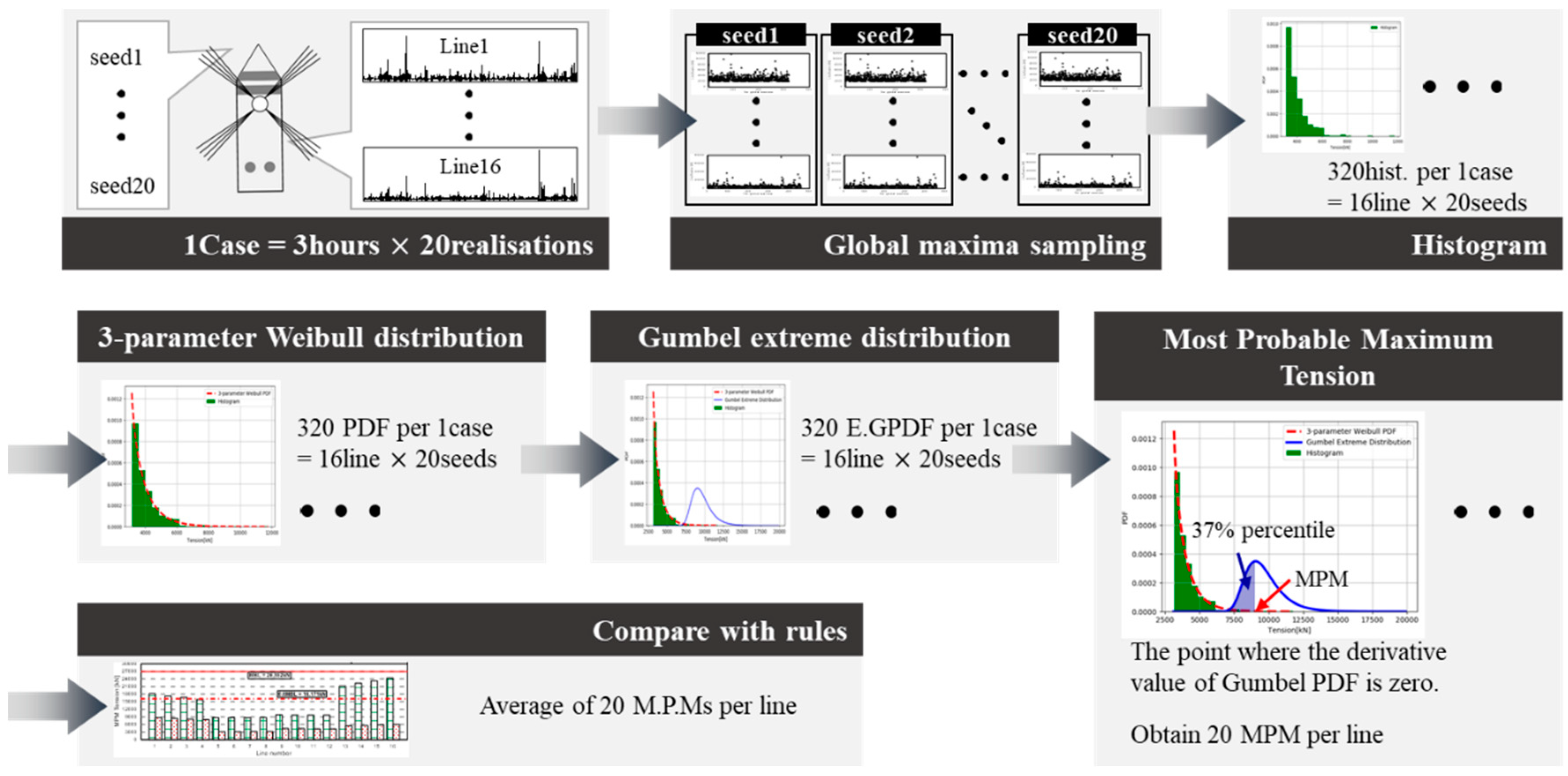
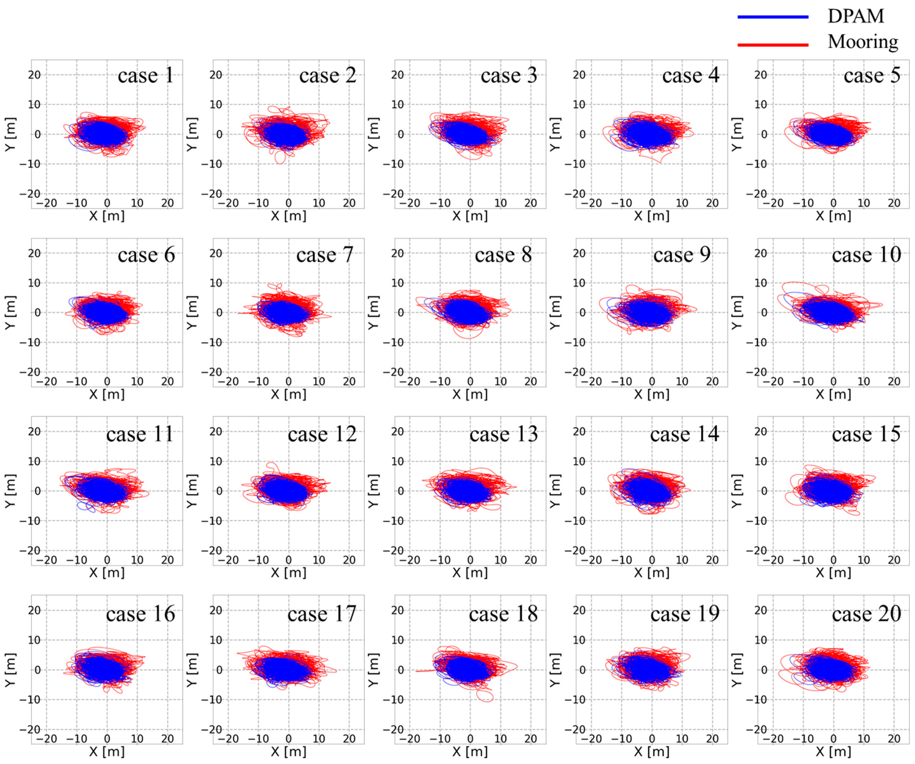
• Time-domain simulations are conducted for 20 different cases with different irregular wave seed under survival or operational condition.
• Global maxima data (mean-up crossing peak value) are sampled from each simulation result.
• The sampled data are rearranged as a probability density function with the 3-parameter Weibull model.
• Since the sampled data are statistically independent, the data are expressed as an extreme distribution by assuming a cumulative distribution function to the power of n. The Gumbel distribution model is recommended for extreme distribution.
• The point at which the tangential slope of the probability density function of the Gumbel extreme distribution is zero is defined as the most MPM value. Twenty MPM values are averaged and compared with the standard of the classification societies, which generally is 60% of MBL.

3. Conditions for the Environment and Simulation

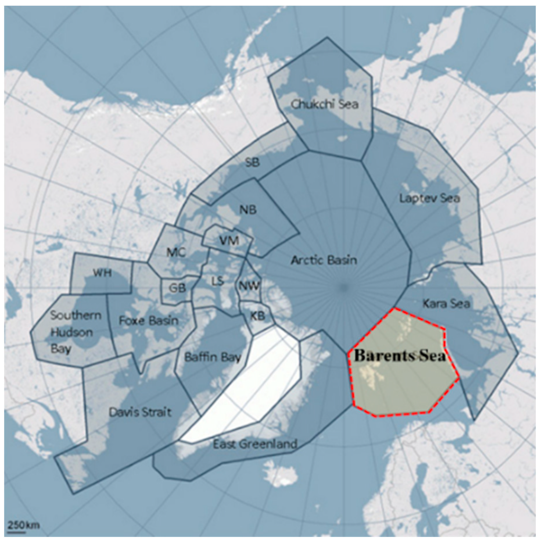
3.1. Information for the Target Site

The Arctic floater in this research is targeted to be used in the Barents Sea, as shown in Figure 4 [23]. The site is selected based on the analysis of the prospects concerning future possible oil and gas development. Even though the average depth of the seawater is about 230 m, the depth is assumed to be 200 m, and it is assumed that the seafloor is flat. The environmental conditions are analyzed from the ocean wave 2012 (GROW2012) data by Ocean Weather, Inc., and the parameters are shown in

Table 1. Environmental parameters for waves, wind, and currents in the Barents Sea by return period.

Return Period (yrs)	Wave			Wind (m/s)	Current (m/s)
	Significant Wave Height (m)	Peak Period (s)	Peakedness Parameter
1	10.30	13.71	2.31	26.03	0.66
10	12.45	14.97	2.39	29.10	0.78
20	13.08	15.34	2.39	29.96	0.82
50	13.91	15.82	2.39	31.06	0.87
100	14.54	16.18	2.39	31.86	0.90

. Metocean data are treated with the extreme value analysis with the 3-parameter Weibull distribution [24]. Regarding the simulation of the survival condition, DNVGL recommends that the return periods for wave, wind, and current be 100, 100, and 110 years, respectively.

3.2. Information on the Floater and DP-Assisted Mooring System

Figure 5 shows the shape of the floater and the approximate arrangement of the station-keeping system used in the research. Both the collision with ice and the production of the hull are considered in the design. Two tunnel type thrusters are located on the bow side, and two azipod type thrusters are placed on the stem side. Considering the environment, an internal turret was selected, and the mooring system consists of four bundles and four lines for each bundle.

Table 2. Particulars for the floater.

Description	Magnitude	Unit
LPP	244	$\left[\mathrm{m}\right]$
Breath	50	$\left[\mathrm{m}\right]$
Draft	18.6	$\left[\mathrm{m}\right]$
Displacement	169614	$\left[{\mathrm{m}}^3\right]$
VCG	19.5	$\left[\mathrm{m}\right]$

provides the details concerning the floater, and the specifications used in the heading control are listed in

Table 3. Specification of DP thrusters.

Turret No.	Type of Thruster	Thrust (kN)	x (m)	y (m)	z (m)
①	tunnel	330	98.3	0	0
②	tunnel	330	93.3	0	0
③	azipod	1600	−105.7	6.5	0
④	azipod	1600	−105.7	−6.5	0

.

The floater had 16 mooring lines with identical characteristics. Each line consists of a chain–wire–chain, and the maximum breaking load (MBL) is 26,952 kN. The pretension is set as 10% of the MBL. The inner bundle angle within a bundle is 2°, and the outer bundle angle is set to be 42°. The radius of the footprint is five times the depth of the water, and the diameter of the turret is 16 m.

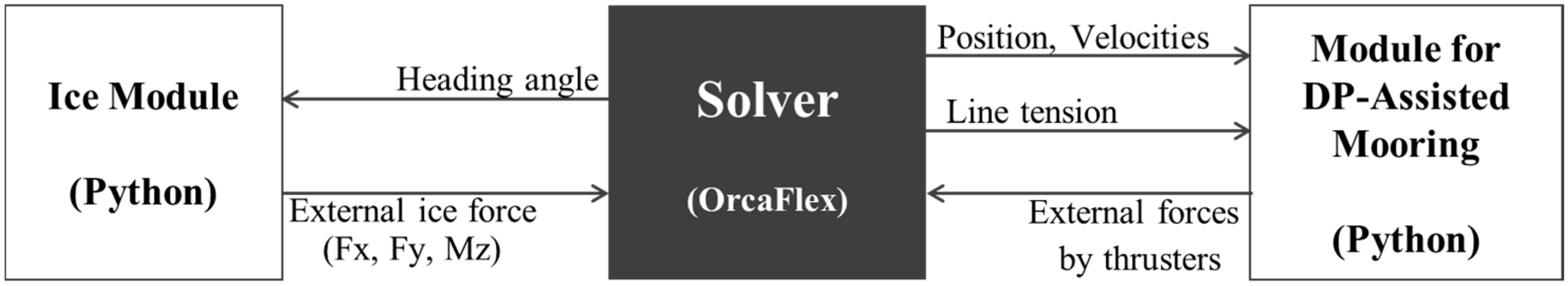
3.3. Simulator Design for the Time-Domain Analysis

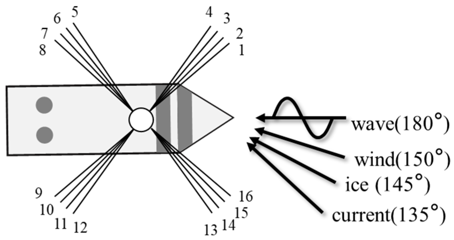
Figure 6 shows the basic concept of time-domain analysis. The ice load and the restoring forces from the DP system are sent to the main solver as external forces. The external modules are made with Python. OrcaFlex is used as the main solver for the time-domain equation of motion. For the DP module, the main solver sends the current position and velocity information. Line tensions are also sent for further investigation. Then, the DP module generates the DP forces to keep the floater within the boundary of the desired position or heading. The procedure to generate the ice load using the ice model is as follows:

• Current heading angle ($\psi$) of the floater is sent from the solver to the ice module for each time step as an input.
• Mean ($\mu \left(\psi \right)$) and standard deviation ($\sigma \left(\psi \right)$) values for $F_x$, $F_y$ and $M_z$ are interpolated for the given angle based on the nine sets of experimental data described in Section 2.3.
• The random value is generated from the probability density function as $X\sim N\left(\mu \left(\psi \right),\sigma {\left(\psi \right)}^2\right)$.
• Remove the resistance term included in the measurement data.
• The ice load that is generated is sent back to the solver and applied to the center of gravity.

The modern trends assume that the ice load against a structure has a form of Weibull distribution [25,26]. Unlike these trends, the results of the experiment were not similar to any type of distribution. Except for some outliers, more than 60% of the data matched normal distribution (See [17] for more details about the dataset.).

3.4. Setup of the Environmental Conditions for the Time-Domain Analysis

The environmental conditions for the simulation are shown in

Table 4. Simulated conditions of the waves, wind, current, and ice.

Wave			Wind	Current	Ice
Hs (m)	Tp (s)	${\rm Y}$	Velocity (m/s)	Velocity (m/s)	Thickness (m)	Length (m)	Speed (m/s)	Concentration	Shape
10.30	13.71	2.31	31.86	0.78	1.4	12	0.514	0.8	irregular

and Figure 7. Generally, the time-domain analysis for the station-keeping system is performed assuming the survival condition, which has a 100-year return period for waves. However, in the Arctic region, harsh waves do not coexist with highly concentrated ice. Therefore, the general survival conditions for waves, winds, and currents with ice are conditions too severe for the floater. This is because of the damping effect that the covered ice has on the wave [27]. Not much research has been completed on how to apply the ice–wave interaction in the motion simulation. In this research, a 1-year return period of the ocean wave selected, and it has the smallest value in Table 1 and is used in the simulation. The 10-year and 100-year return periods are applied for the current and wind, respectively, as directed by DNVGL. The ice parameters are the same values used in the ice tank experiment. The ARC 7 condition of the Russian Maritime Register of Shipping is considered in deciding the parameters.

The directions of the loads are set according to the DNVGL standard for the non-collinear condition. Waves are from the head sea, and the wind and current are applied to the floater at 30° and 45° angles with respect to the wave. The direction of the ice is not well defined for the time-domain simulation. As mentioned earlier, it is assumed that the ice drifts between the current and wind directions.

4. Simulation Results

Simulation is conducted for the floater using the system described in Section 3.3 based on the environmental conditions in Section 3.4. The heading control mode is selected for the DP system in order to reflect the difficulties associated with the on-site operation of the DP vessel in the ice-covered sea. The target heading is set to be against the direction of the ice drift. According to the DNVGL standard, 20 seeds are selected randomly for the irregular waves, and a 3-h time-domain simulation is conducted for each seed.

Figure 8 is an example to show the effect of ice loads on the station-keeping performance. Simulation results were compared for a total of four cases, with and without ice and DP for the same environmental conditions. As mentioned earlier, the MPM value is the point at which the cumulative value is 37% of the Gumbel probability density function. Therefore, the smaller circles indicate that the floater stays mostly within a smaller boundary. The maximum offset under no ice condition is 9.9 m, whereas the one under ice condition is 16.8 m. With the ice, the MPM value is 10.1 m without ice and 15.1 m with ice. The result indicates the significance of ice-induced forces on the station-keeping of the given floating structure in an ice-covered sea.

Figure 9 shows the trajectories of the floater in 3-h simulations for both the DPAM and mooring only scenarios. Since the same seed gives the same phases and consequently the same train of waves, two simulations are run for a single seed, i.e., one for DPAM and another for the mooring-only scenario. This was repeated 20 times with 20 different seeds. Since the actual number of seeds was selected randomly in this research, the results were organized as case 1 to case 20 for easy identification.

The allowable offset was set as 20 m, which was 10% of the depth of the water. For the mooring-only system, in some cases, the position approached the limit boundary (i.e., case 18, case 20, and others). With the heading control by DPAM, the trajectory of the floater remained stably within the allowable offset.

Figure 10 shows circles by setting the radius to be the maximum offset during the 3-h simulation. This enables the identification and comparison of the performances of the two scenarios. The circles in Figure 11 are the MPM values after the statistical process for the performance evaluation for three hours.

In some cases, the difference in the maximum offset is small (case 3, case 6). This is because the environment is relatively mild, and the mooring-only system works fine. In some cases, i.e., when the offset is large due to the severe environmental loads, the difference is relatively small. This is due to a freak wave, which is a much larger wave than the height of a significant wave. With such a rogue wave, the DP system cannot work effectively against the environment.

Table 5. Reduction rate of the difference values of maximum offset and MPM values between DPAM and mooring-only systems ((DPAM value—mooring-only value)/20 $\times$ 100%).

Case No.	1	2	3	4	5	6	7	8	9	10	11	12	13	14	15	16	17	18	19	20
maximum offset (%)	9	19	5	12	13	3	30	15	13	9	9	19	22	9	23	13	29	29	10	17
MPM (%)	14	25	11	11	17	9	20	15	17	17	14	18	23	16	16	12	23	19	11	19

shows the improvement in the performance of DPAM over the mooring-only system. The numbers show the rate of improvement with respect to the allowable offset of 20 m. The mean value in terms of the maximum offset is 15.4% (3.1 m).

Figure 12 shows the MPM values of line tension for each simulation case. The environmental loads are applied to the top, left direction as shown in Figure 7, and the mooring lines in bundle 2 show the least values in the mooring only scenario. Since the angle of the inner bundle is small, the tensions in that bundle have similar values, and the MPM values also are almost identical. Therefore, the average value of the mooring lines in the same bundle can be used as a representative MPM value, and the mean MPM values are computed for each bundle in each of the simulation cases.

Table 6. Reduction rate ¹ of tension MPM with respect to the maximum breaking loads.

Case No.	1	2	3	4	5	6	7	8	9	10	11	12	13	14	15	16	17	18	19	20
Bundle 1	9	25	5	5	21	15	12	16	14	12	15	12	16	22	16	5	12	7	19	22
Bundle 2	9	9	7	5	5	4	4	3	3	6	3	1	5	4	4	−1	9	3	4	7
Bundle 3	29	24	26	21	26	23	26	27	24	30	23	21	30	22	23	20	18	19	15	19
Bundle 4	20	28	19	11	24	11	21	19	20	27	22	19	26	23	22	13	31	19	20	27

¹$\left(MooringMPM-DPAMMPM\right)÷0.6MBL\times 100[\%]$.

summarizes the reduction rate and shows how much the MPM values were reduced for the two scenarios. The difference of the MPM values for mooring-only and DPAM is divided by the allowable load, which is 60% of MBL. The results are shown schematically in Figure 13.

The reduction rates for bundles 1, 2, 3, and 4 were 6.7%, 1.8%, 9.2%, and 8.8%, respectively. Bundle 2 had the smallest reduction rate, i.e., 1.8%, but the other three bundles had an average reduction rate of 8.3%, so the average reduction rate for all four bundles was 6.6%. Regarding the direction of complex environmental loads, severe situations occurred mainly in the left-half plan. Therefore, the reduction rate for bundle 2 was relatively small, and the heading control can reduce the tension significantly for the lines in bundle 4. Bundle 3 also had a large reduction rate. This was due to the restoring forces provided by the mooring lines, which induced significant movement to the right side and resulted in the tendency of the environmental loads moving to the north side. Note that the values show the improvement that was made by the heading control of DPAM. Therefore, heading control can reduce the severe tensions significantly for bundle 3 and bundle 4.

Figure 14 shows the variation of the heading angles for each case. The target heading was set at −35°, which is the opposite direction from the drifting ice. The simulation results show that the heading control worked well and maintained the desired heading angle for the DPAM while showing a large fluctuation of the heading angle in the case of the scenario of mooring-only. Therefore, heading control can contribute both to tension control and position control by reducing the fluctuation of the heading angle, thereby resulting in a small drift against complex environmental loads, including ice-induced forces.

5. Conclusions and Future Work

The effect of the heading control by the DP system was investigated for an Arctic floating structure. Based on the experimental data acquired using the ice tank at KRISO, an ice load was generated using a statistical process. Then, the ice force that was generated and applied to the specially designed structure, along with waves, winds, and currents, as components of complex environmental loads. The motion of the floater was analyzed for the conditions at the target site. Two scenarios were tested, i.e., the DPAM and the mooring-only system, and the results were compared. The heading control mode was set for DPAM, and 3-h time-domain simulations were conducted. The MPM values of the position offset and the line tension for both scenarios were derived from the results and compared to verify the effectiveness of the heading control. The main observations are summarized below:

• The functionalities of the ice load generation module and the DP force generation module were verified and applied to the time-domain analysis with a motion solver. These modules can be used to further assess various scenarios in harsh environmental conditions.
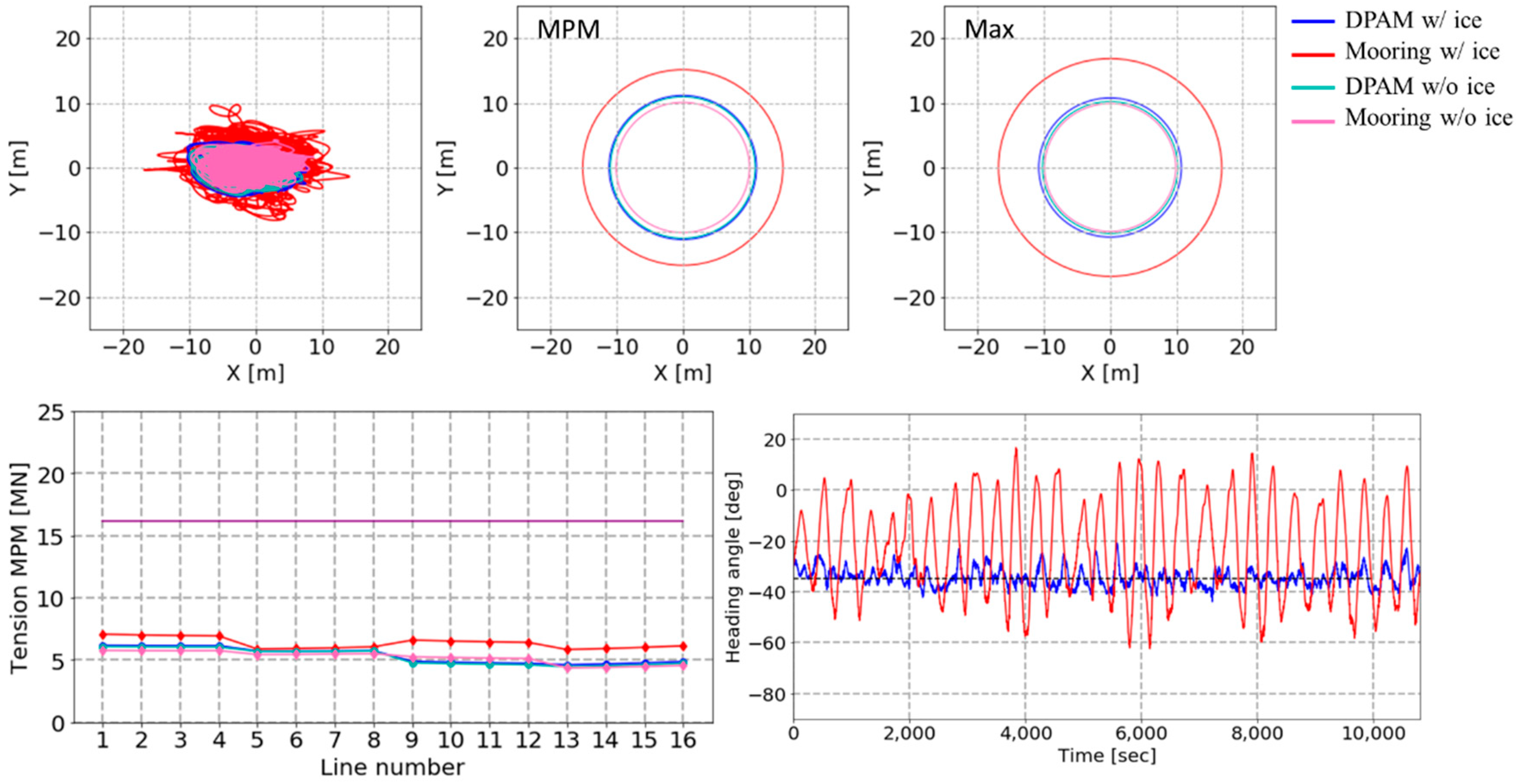
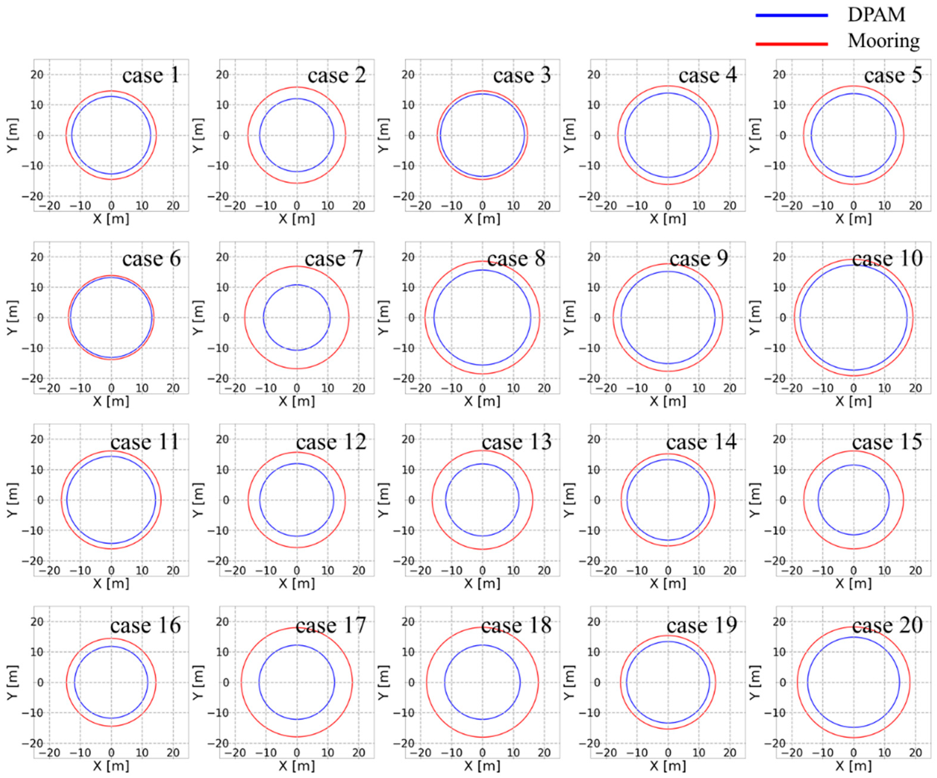
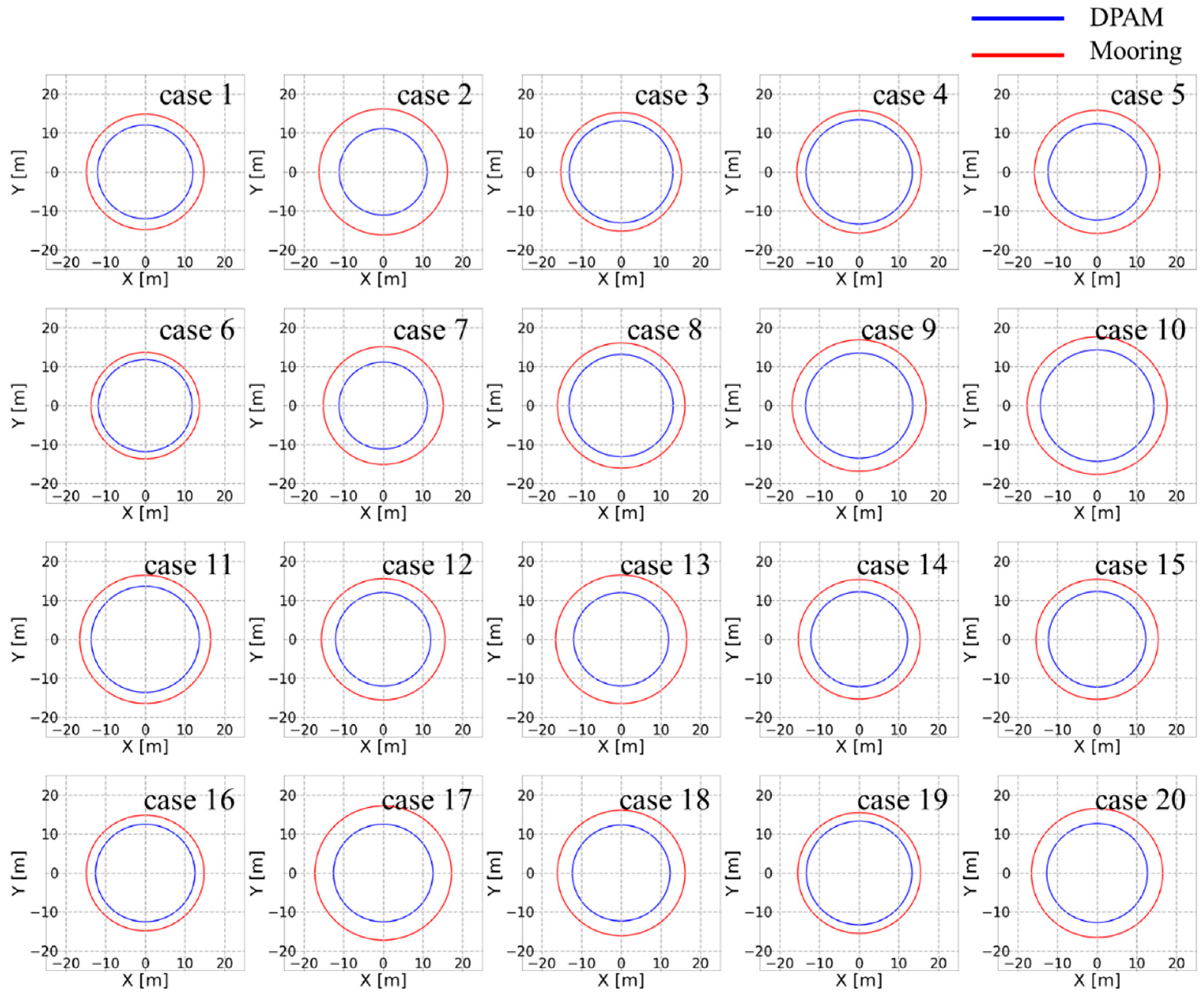
• With the DPAM heading control, the maximum position offset was reduced to 3.1 m (15.4% of the allowable maximum offset of 20 m) based on the average of the 20 cases. The mean value for the reduction of MPM was about 3.3 m (16.3%). The target heading angle was set in the ice drift direction, which was between the wind and current directions. Therefore, the station-keeping performance was enhanced by reducing the drift of complex environmental loads.
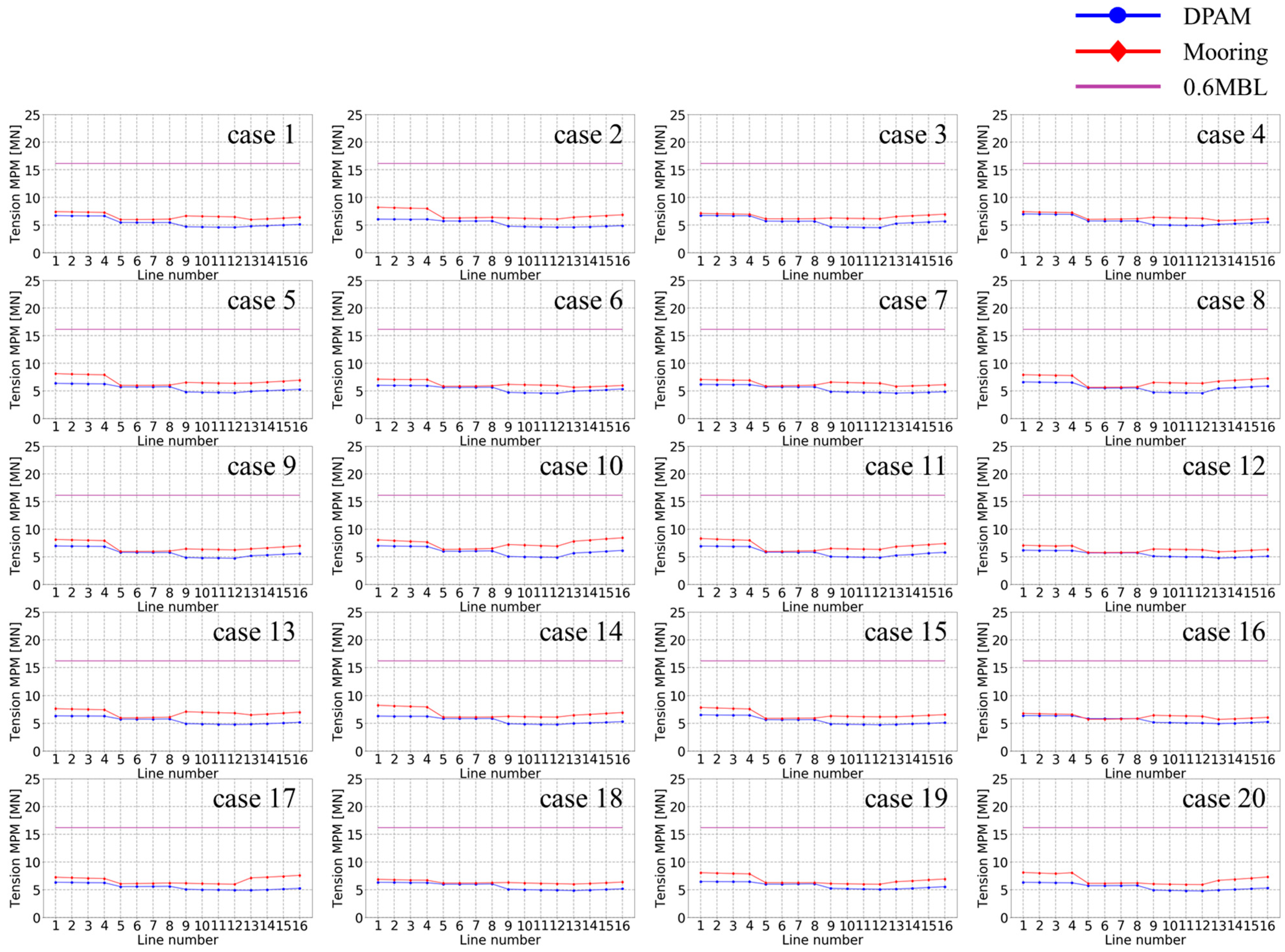
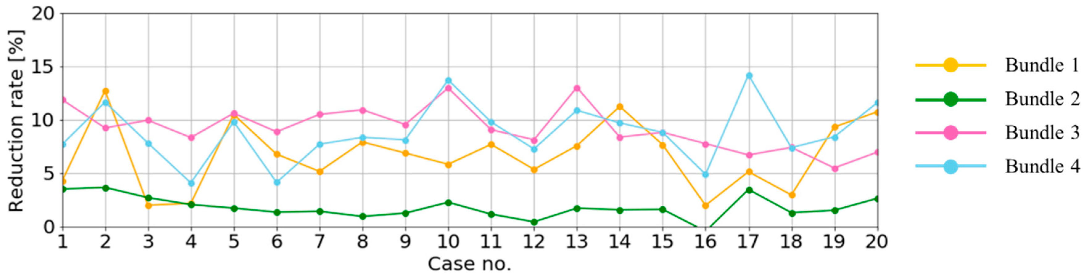
• Except for bundle 2, which had the smallest tensions due to its configuration, the MPM values were reduced by 8.2% with respect to the 0.6 MBL, which was the design criterion Heading control reduces the beam sea situation and lowers the tension on the mooring lines due to the smaller floater motion.

The results of this research are expected to be used in redesigning the mooring lines when the Arctic floater is equipped with a DP system. The following items will be investigated further:

• It is necessary to consider the coupled effect between an ice load and other environmental loads. When the heading angle is larger than a certain limit, the DP thrusters cannot generate an adequate restoring force. This effect cannot be considered by the current module used to generate the ice load. Therefore, a more precise ice module will be developed.
• The direction of the heading control is set such that it is the opposite of the drift direction of the ice floe. This is to consider the significance of the ice load, but the direction may not be the dominant direction in which the floater must be controlled. PID control may have limitations on this issue, and more-complicated, active-type controllers will be studied.
• Further investigation is necessary to determine the relationship between the condition of the ice and a wave. This study considered a 1-year return period (for a significant wave height of 10.3 m), but the condition is still too harsh for the ice field with 80% concentration. Feasible environmental conditions will be analyzed for realistic motion analysis in the time domain.
• As data related to structural design have yet to be prepared, no analysis of vibration was conducted. Further research is necessary because vibration studies related to natural frequencies are essential for the designed floater.

References

1. Zhou, L.; Moan, T.; Riska, K. Heading control for turret-moored vessel in level ice based on Kalman filter with thrust allocation. J. Mar. Sci. Tech. 2013, 18, 460–470. [Google Scholar] [CrossRef]
2. Ansari, K.A. Effect of vessel hydrodynamic mass on the station-keeping response of a moored offshore vessel. Trans. ASME 1989, 108, 52–58. [Google Scholar] [CrossRef]
3. Choung, J.; Jeon, G.-Y.; Kim, Y. Study on Effective Arrangement of Mooring Lines of Floating-Type Combined Renewable Energy Platform. J. Ocean Eng. Tech. 2013, 27, 22–32. [Google Scholar] [CrossRef] [Green Version]
4. API, D. Analysis of Stationkeeping Systems for Floating Structures; API-RP-2SK.; American Petroleum Institute: Washington, DC, USA, 2005. [Google Scholar]
5. Moran, K.; Backman, J.; Farrell, J.W. Deepwater drilling in the Arctic Ocean’s permanent sea ice. Proc. Int. Ocean Drill. Program 2006, 302, 2. [Google Scholar]
6. Liferov, P.; Serre, N.; Kerkeni, S.; Bridges, R.; Guo, F. Station-Keeping Trials in Ice: Test Scenarios. In Proceedings of the ASME 2018 37th International Conference on Ocean, Offshore and Arctic Engineering, Madrid, Spain, 17–22 June 2018; American Society of Mechanical Engineers: New York, NY, USA, 2018. [Google Scholar]
7. Kerkeni, S.; Liferov, P.; Serre, N.; Bridges, R.; Jorgensen, F. Station-Keeping Trials in Ice: Dynamic Positioning in Ice-Results and Learnings. In Proceedings of the ASME 2018 37th International Conference on Ocean, Offshore and Arctic Engineering, Madrid, Spain, 17–22 June 2018; American Society of Mechanical Engineers: New York, NY, USA, 2018. [Google Scholar]
8. Jenssen, N.A.; Hals, T.; Jochmann, P.; Haase, A.; dal Santo, X.; Kerkeni, S.; Doucy, O.; Gürtner, A.; Støle Hetschel, S.; Moslet, P.O.; et al. DYPIC—A Multi-National R&D Project on DP Technology in Ice. In Proceedings of the Dynamic Positioning Conference, Houston, TX, USA, 9 October 2012. [Google Scholar]
9. Kerkeni, S.; Santo, X.D.; Doucy, O.; Jochmann, P.; Haase, A.; Metrikin, I.; Løset, S.; Jenssen, N.A.; Hals, T.; Gürtner, A.; et al. DYPIC project: Technological and scientific progress opening new perspectives. In Proceedings of the OTC Arctic Technology Conference, Houston, TX, USA, 13 February 2014. [Google Scholar]
10. Wang, J.; Sayeed, T.; Millan, D.; Gash, R.; Islam, M.; Millan, J. Ice Model Tests for Dynamic Positioning Vessel in Managed Ice. In Proceedings of the Arctic Technology Conference, St. John’s, NL, Canada, 24–26 October 2016. [Google Scholar]
11. Lubbad, R.; Løset, S.; Lu, W.; Tsarau, A.; van den Berg, M. An overview of the Oden Arctic Technology Research Cruise 2015 (OATRC2015) and numerical simulations performed with SAMS driven by data collected during the cruise. Cold Reg. Sci. Technol. 2018, 156, 1–22. [Google Scholar] [CrossRef]
12. Lubbad, R.; Løset, S.; Lu, W.; Tsarau, A.; Van Den Berg, M. Simulator for arctic marine structures (SAMS). In Proceedings of the ASME 2018 37th International Conference on Offshore Mechanics and Arctic Engineering—OMAE, Madrid, Spain, 17 June 2018. [Google Scholar]
13. Raza, N.; van der Berg, M.; Lu, W.; Lubbad, R. Analysis of Oden Icebreaker Performance in Level Ice using Simulator for Arctic Marine Structures (SAMS). In Proceedings of the 25th International Conference on Port and Ocean Engineering under Arctic Conditions, Delft, The Netherlands, 9–13 June 2019. [Google Scholar]
14. Daley, C.; Alawneh, S.; Peters, D.; Quinton, B.; Colbourne, B. GPU Modeling of Ship Operations in Pack Ice. In Proceedings of the International Conference and Exhibition on Performance of Ships and Structures in Ice, Banff, AB, Canada, 17–20 September 2012. [Google Scholar]
15. Daley, C.G.; Alawneh, S.; Peters, D.; Blades, G.; Colbourne, B. Simulation of Managed Sea Ice Loads on a Floating Offshore Platform using GPU-Event Mechanics. In Proceedings of the International Conference and Exhibition on Performance of Ships and Structures in Ice IceTech, Banff, AB, Canada, 28–31 July 2014. [Google Scholar]
16. Kim, Y.-S.; Kim, J.-H.; Kang, K.-J.; Han, S.; Kim, J. Ice Load Generation in Time Domain Based on Ice Load Spectrum for Arctic Offshore Structures. J. Ocean Eng. Tech. 2018, 32, 411–418. [Google Scholar] [CrossRef]
17. Kang, H.H.; Lee, D.; Lim, J.; Lee, S.J.; Jang, J.; Jung, K.; Lee, J. Development of Ice Load Generation Module to Evaluate Station Keeping Performance for Arctic Floating Structures in Time Domain. J. Ocean Eng. Tech. 2020, 34, 394–405. [Google Scholar] [CrossRef]
18. Ghafari, H.; Dardel, M. Parametric study of catenary mooring system on the dynamic response of the semi-submersible platform. Ocean Eng. 2018, 153, 319–332. [Google Scholar] [CrossRef]
19. Orcaflex Morison Elements. Available online: https://www.orcina.com/webhelp/OrcaFlex/Content/html/Morisonelements.htm (accessed on 20 December 2020).
20. Trunbull, I.D.; Torbati, R.Z.; Taylor, R.S. Relative influences of the metocean forcings on the drifting ice pack and estimation of internal ice stress gradients in the Labrador Sea. J. Geophys. Res. Oceans 2017, 122, 5970–5997. [Google Scholar] [CrossRef]
21. DNV, G.L. Offshore Standard: Position Mooring; DNVGL-OS-E301; DNV GL: Oslo, Norway, 2015. [Google Scholar]
22. Veritas, B. Classification of Mooring Systems for Permanent and Mobile Offshore Units; NR-493-DT-R03-E; BV: Neuilly sur Seine, France, 2015. [Google Scholar]
23. IUCN/SSC PBSH Barents Sea (BS). Available online: http://pbsg.npolar.no/en/status/populations/barents-sea.html (accessed on 20 December 2020).
24. Park, S.B.; Shin, S.Y.; Shin, D.G.; Jung, K.H.; Choi, Y.H.; Lee, J.; Lee, S.J. Extreme Value Analysis of Metocean Data for Barents Sea. J. Ocean Eng. Technol. 2020, 34, 26–36. [Google Scholar] [CrossRef]
25. Kujala, P.; Suominen, M.; Riska, K. Statistics of Ice Loads Measured on Mt Uikku in the Baltic. In Proceedings of the 20th International Conference on Port and Ocean Engineering under Arctic Conditions, Luleå, Sweden, 9–12 June 2009. [Google Scholar]
26. Suominen, M.; Kujala, P.; Romanoff, J.; Remes, H. Influence of load length on short-term ice load statistics in full-scale. Mar. Struct. 2017, 52, 153–172. [Google Scholar] [CrossRef]
27. Sutherland, B.R.; Balmforth, N.J. Damping of surface waves by floating particles. Phys. Rev. Fluids 2019, 4, 010804. [Google Scholar] [CrossRef]
Figure 1. General form of a dynamic positioning (DP) control system.
Jmse 09 00102 g001
Figure 2. (a) Model of a dynamic mooring line; (b) free body diagram for a Morison element.
Jmse 09 00102 g002
Figure 3. Statistical process to calculate most probable maxima (MPM) from the time history of line tensions.
Jmse 09 00102 g003
Figure 4. Location of Barents Sea in the Arctic.
Jmse 09 00102 g004
Figure 5. (a) Shape of the hull of the floating structure; (b) arrangement of the DP thrusters and mooring lines for the DP assisted mooring system.
Jmse 09 00102 g005
Figure 6. Dynamic motion analysis with ice and DP modules in the time domain with a motion solver.
Jmse 09 00102 g006
Figure 7. Directions of the complex environmental loads.
Jmse 09 00102 g007
Figure 8. The comparison of station-keeping performance to analyze the effects of ice loads.
Jmse 09 00102 g008
Figure 9. Trajectories of the floater for a 3-h simulation. Dynamic positioning assisted mooring (DPAM) and mooring only systems were compared with the same seed. Simulations were repeated for 20 different seeds.
Jmse 09 00102 g009
Figure 10. Circles with radii representing the maximum offset for each simulation.
Jmse 09 00102 g010
Figure 11. Circles representing MPM values for the offset of the structure.
Jmse 09 00102 g011
Figure 12. MPM values of the tensions of the mooring lines; the 60% maximum breaking load (MBL) lines are drawn as a criterion.
Jmse 09 00102 g012
Figure 13. Graphical representation of the rate of reduction of the tension.
Jmse 09 00102 g013
Figure 14. Time history of the heading angles for a 3-h simulation.
Jmse 09 00102 g014