Abstract
Machine learning tools are increasingly adopted in various industries because of their excellent predictive capability, with high precision and high accuracy. In this work, analytical equations to predict the failure pressure of a corroded pipeline with longitudinally interacting corrosion defects subjected to combined loads of internal pressure and longitudinal compressive stress were derived, based on an artificial neural network (ANN) model trained with data obtained from the finite element method (FEM). The FEM was validated against full-scale burst tests and subsequently used to simulate the failure of a pipeline with various corrosion geometric parameters and loadings. The results from the finite element analysis (FEA) were also compared with the Det Norske Veritas (DNV-RP-F101) method. The ANN model was developed based on the training data from FEA and its performance was evaluated after the model was trained. Analytical equations to predict the failure pressure were derived based on the weights and biases of the trained neural network. The equations have a good correlation value, with an R2 of 0.9921, with the percentage error ranging from −9.39% to 4.63%, when compared with FEA results.
1. Introduction
Pipelines are the most economical means of transport between gas wells, storage facilities, refinery plants and power plants. Failure of pipelines may pose catastrophic consequences to their surroundings, on top of economic losses from production interruption. Pipelines are susceptible to compressive longitudinal loads due to hoop stress from internal pressure and thermal stress induced by thermal expansion and pipe–soil friction resistance [1]. Corrosion is a significant cause of pipeline failure as it thins the pipe wall, weakening the structural integrity of the pipeline by reducing the load-carrying capacity of the pipeline due to stress concentration at the corrosion region [2].
Formation of corrosion in a pipeline is often irregular and unpredictable, with different types of corrosion formation having different structural effects on a pipeline. A corrosion defect disrupts the stress and strain field of a pipeline beyond the defect. A single corrosion defect has zero or negligible interactions with other corrosion defects, provided that the distance between these defects is outside of the interaction limit. Corrosion defects usually occur as clusters of corrosion pits, with a complex defect geometry rather than a single uniform defect. Interacting defects are more detrimental towards the structural integrity of a pipeline than single defects, as they may interact with each other and reduce the failure capacity of the pipeline [3]. Therefore, they need to be considered differently when assessing corroded pipelines. Corrosion defects are commonly categorised and assessed by the type of interaction. For example, longitudinally aligned groups of corrosion defects have a Type 2 interaction, where defects lie on the same axial line and are separated by a length of pipe wall thickness. DNV defines the interaction limit of longitudinal interacting defects as per Equation (1), as a function of the outer diameter D and thickness t of a pipe [4]. Defect spacing s equal or greater than the interaction limit will be treated as a single defect, due to the negligible interaction effect [5].
Residual strength assessment of a corroded pipeline can be assessed based on different complexities. ASME B31G classifies the complexity of assessment from Level 0 to Level 3 [6]. Level 0 assessment relies on the tables of allowable defect depth and length. Level 1 assessment is a simple calculation based on defect depth and length, usually used by personnel in the field. The Level 2 assessment method is a calculation that incorporates a greater detail of information than Level 1 to produce a more accurate estimate of the failure pressure. It relies on detailed measurements of the corroded surface profile and involves repetitive calculations. The Level 3 assessment method requires the specifics of the corrosion defects such as their geometries, loadings, boundary conditions, material properties and failure criteria.
Considerable progress has been made recently to improve Level 2 and Level 3 assessments. It is known that Level 2 assessments based on established standards and codes, such as ASME B31G [6], RSTRENG Effective Area [7] and DNV RP-F101 [4], are conservative in their estimation [8]. These assessment standards are limited in their capabilities and most of them are applicable to a corroded straight pipeline with a single corrosion defect subjected to internal pressure only. Numerous works have been conducted to improve their predictions and expand their limited scope. Khalajestani et al. revised DNV’s equation and expanded its capability to assess single-defect corrosion at the intrados, crown and extrados of pipe elbows [9]. FEA results from Level 3 assessment were utilised to develop a new assessment model that considered different defect geometries and configurations [10,11], boundary conditions and loadings [12] and different material properties [13]. The reliability of conventional assessment methods such as DNV was improved by redefining the defect depth of DNV’s equations [14]. A new assessment model was developed by using numerical tools such as Monte Carlo simulation (MCS) to establish and solve limit state equations [15]. A proprietary program, PIPEFLAW, is able to quickly assess the integrity of corroded pipelines. The programme is considered a Level 4 assessment method as it can automatically generate and analyse corroded pipeline models subjected to internal pressure and axial compressive force [16,17].
Of all the established residual strength assessment standards, DNV RP-F101 is the most comprehensive method, as it is applicable to corroded pipelines with a single defect (subjected to internal pressure and longitudinal compressive stress) and longitudinally interacting defects (subjected to internal pressure only). Equation (2) from the DNV guidelines is used to determine the failure pressure of a pipe with a single corrosion defect under combined loads of internal pressure and longitudinal compressive stress. Equation (2) is the product of Equations (3) and (4), where Equation (3) is used to determine the failure pressure of a pipe with a single corrosion defect under internal pressure only and Equation (4) gives the factor for longitudinal compressive stresses.
However, Level 2 assessment methods have varying degrees of accuracy in their prediction of the failure pressure when compared to Level 3 assessment methods such as numerical analysis using the finite element method [18]. Level 3 assessment methods involve advance analysis techniques and require a higher level of information such as boundary conditions and material properties for the analysis. Numerical methods such as the finite element method (FEM) have been widely employed to verify and validate the failure behaviour and failure pressure of corroded pipelines [17,19,20,21]. FEM is especially useful for parametric studies with varying corrosion geometries, which otherwise would be too costly to be carried out experimentally. Despite the advantages of Level 3 assessment methods, numerical methods are computationally expensive. One FEM simulation with upwards of thirty thousand nodes in a model may take up to two to three hours. A comprehensive parametric study for varying corrosion defect geometries through FEM can be computationally and time-intensive.
Machine learning has been increasingly adopted for assessing the integrity and reliability of corroded pipelines. Machine learning models have been developed to predict the burst pressure of corroded pipelines, trained with a database of corroded pipeline burst pressures determined experimentally [22,23,24]. Machine learning techniques could be used to develop a new assessment method that combines the advantages of both Level 2 and Level 3 assessment methods. Data-driven machine learning frameworks such as artificial neural networks (ANNs) have been used in the past to predict the failure pressure of straight pipes and pipe bends with a single corrosion defect [9,25], as well as interacting corrosion defects [5,10]. The dataset used to train the ANN models was derived from the FEM and full-scale burst test of pipelines with machined defects. These ANN models were used to understand the non-linear relationship between the corrosion geometries and failure pressure of corroded pipelines when subjected to internal pressure only. Tohidi and Sharifi [26] found that the weights and biases from a trained ANN can be used to formulate an equation for the ultimate strength of locally corroded plate girder ends. The formula has a high degree of accuracy and can be used readily.
This paper proposes the application of an ANN together with the FEM to formulate an equation to predict the failure pressure of a corroded pipeline with varying longitudinally interacting corrosion defect geometries, subjected to internal pressure and longitudinal compressive stress.
2. Materials and Methods
In this paper, finite element analysis (FEA) was conducted on an API 5L X65 grade steel pipeline with longitudinal corrosion defects, subjected to combined loads of internal pressure and longitudinal compressive stress. The FEM was validated with experimental results from full-scale burst tests to ensure an accurate representation of the material property, element types and mesh configurations. A database of FEA results was generated with various corrosion geometric parameters and load applications and used to train an ANN model. The weight and biases of the trained ANN were subsequently used as a basis to formulate an equation to predict the failure pressure of a corroded pipeline with varying longitudinally interacting corrosion defect geometries, subjected to internal pressure and longitudinal compressive stress.
2.1. Finite Element Method
The FEA was conducted using ANSYS (19.1) Mechanical APDL. The base pipe model had an external diameter De of 300 mm, a wall thickness t of 10 mm and a length L of 2000 mm. The shape of the corrosion defect was rectangular, with varying defect depths, defect lengths and defect widths, as shown in Table 1. The corrosion defects were spaced longitudinally, as shown in Table 1. The range of longitudinal compressive stress (as a ratio of API 5L X65’s yield strength) considered is shown in Table 1.

Table 1.
Parameters of corrosion defect geometries and external load.
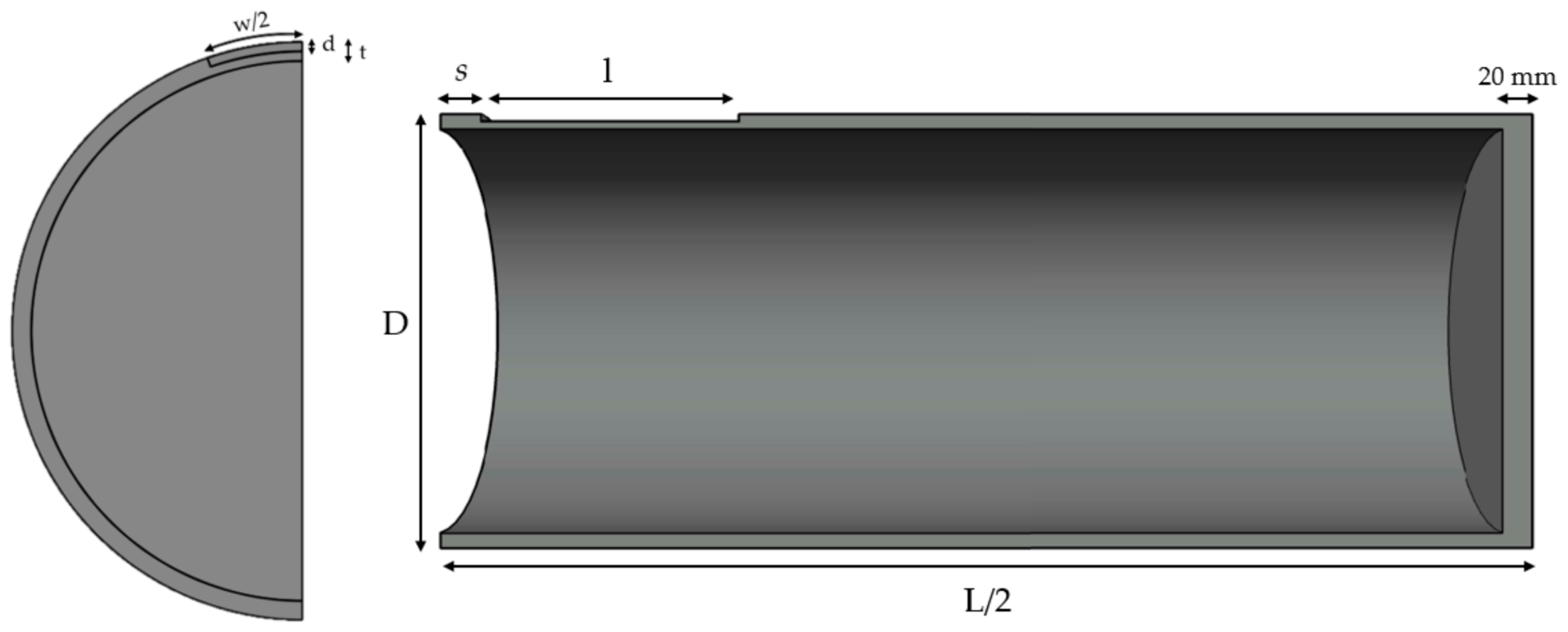
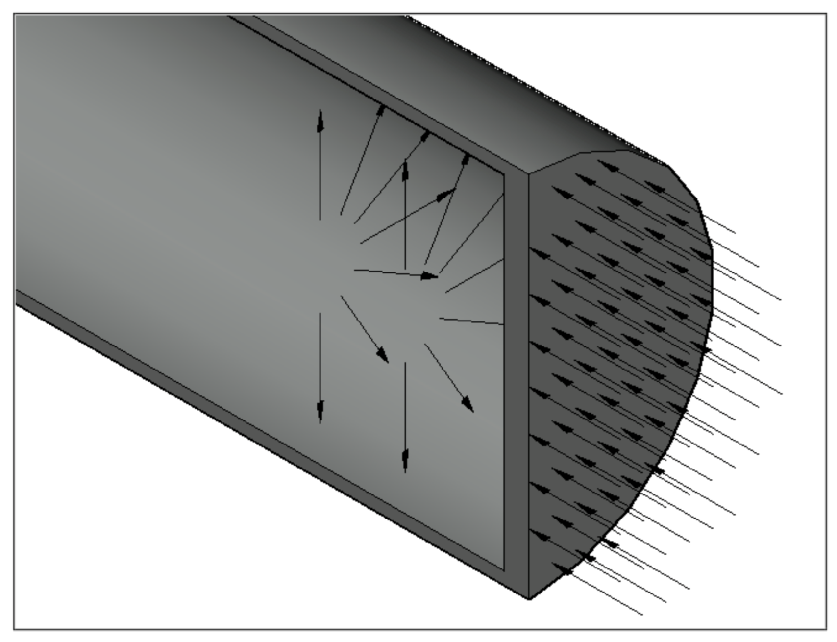
Only a quarter model was simulated in the FEA, as the pipe and corrosion defects were assumed to be symmetrical, therefore reducing the computational time. Figure 1 illustrates the quarter pipe and its dimensions. Internal pressure was applied on the inner surface of the pipe and end cap, whereas longitudinal compressive stress was applied on the surface of the end cap, as shown in Figure 2. The longitudinal compressive stress was applied incrementally through ramped loading in ANSYS from the first timestep. An internal pressure was then applied in the second timestep, while the longitudinal compressive stress was maintained.
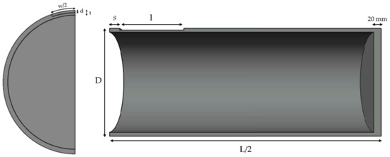
Figure 1.
Dimensions of the quarter pipe model.
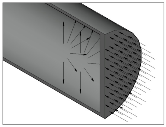
Figure 2.
Loads applied on the pipe model.
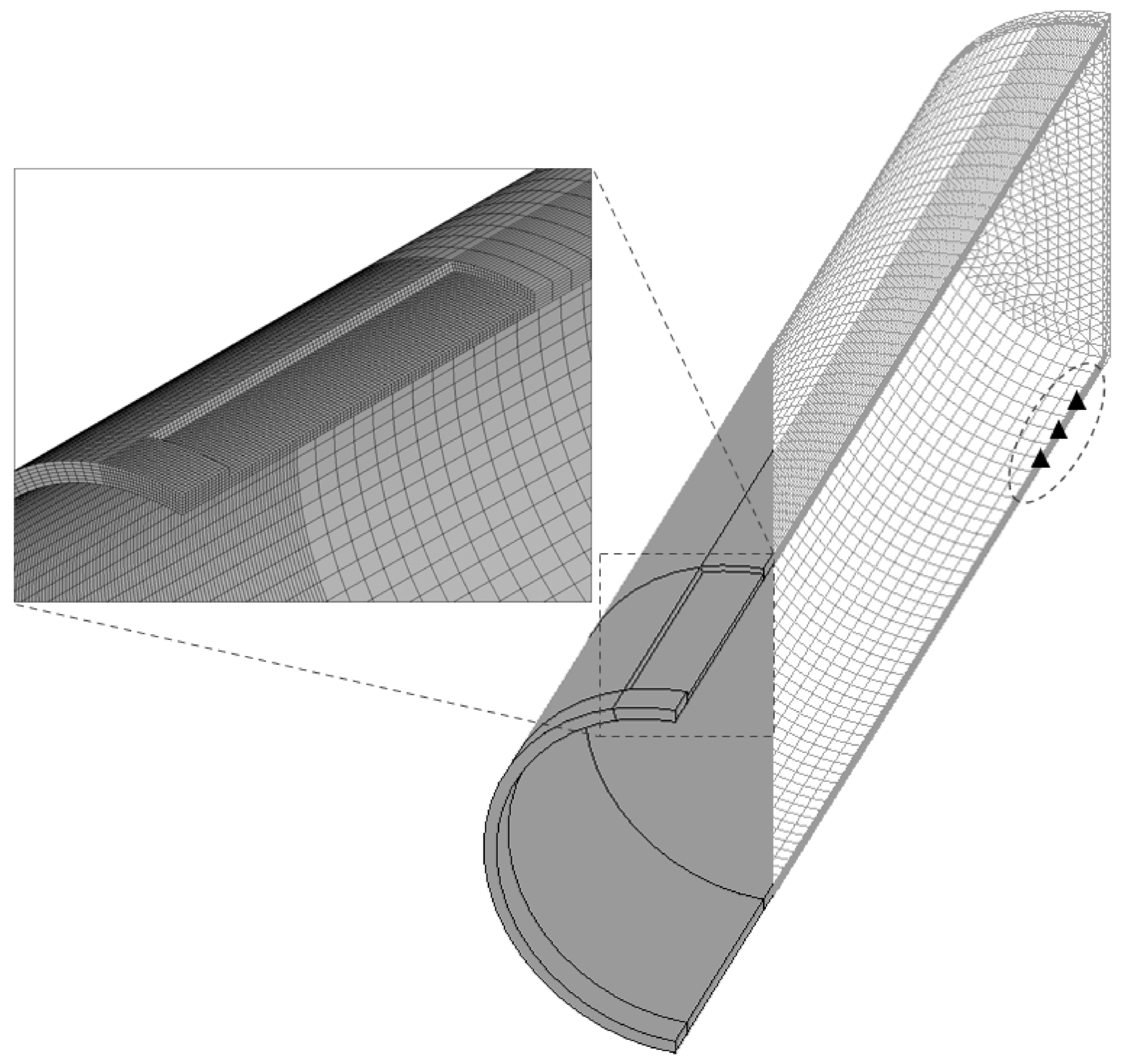
The pipe body was brick meshed with an 8-node SOLID185 element in ANSYS, while the end cap was free meshed with a 20-node SOLID186 element. Both elements support plasticity, stress stiffening, large deflection and large strain capabilities, and thus they are suitable for simulating deformations of elastoplastic materials such as API 5L X65 steel pipelines. However, SOLID186 is more suited for modelling irregular meshes of curved boundaries at the end cap. Three layers of elements were meshed at the corrosion defect, as per the British Standards Institution recommendation [27]. The model was constrained in its position to prevent rigid motion during FEA. The movement of three nodes near the end cap was restricted, as indicated in Figure 3 [28]. The corrosion defect was densely packed with elements. The density of elements reduced gradually away from the corrosion defect, as shown in Figure 3. Mesh convergence was performed to determine the optimal mesh density.
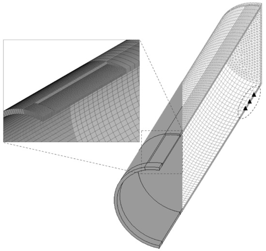
Figure 3.
Pipe model with a longitudinally interacting corrosion defect.
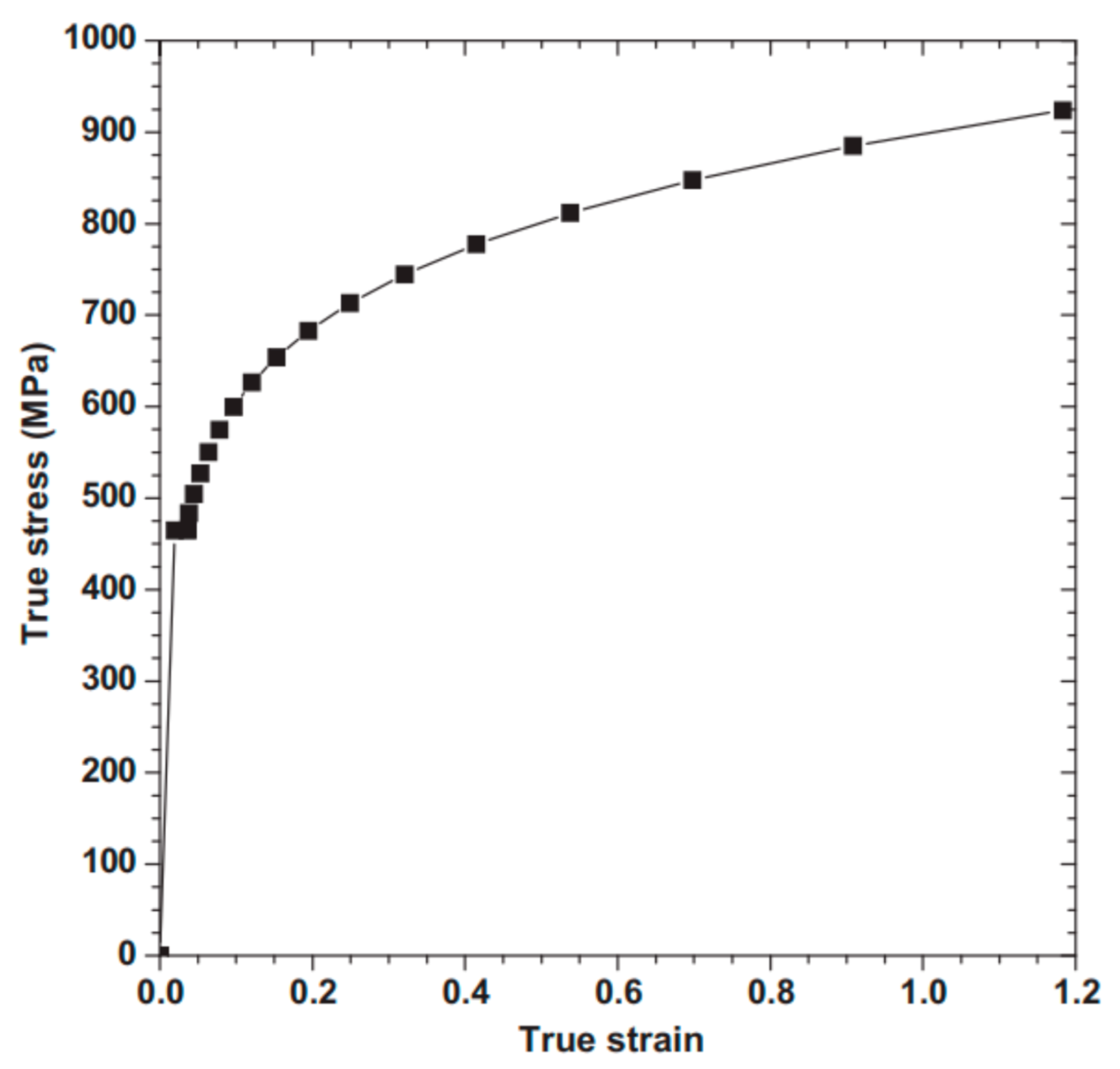
The material property of the API 5L X65 grade steel pipe from Baek et al.’s work [29] was adapted for this study, as shown in Figure 4. The non-linear true stress–strain curve of API 5L X65 was used as the material property of the pipe body in SOLID185 elements. Static non-linear structural analysis (Newton–Raphson) was used in the FEM to account for the non-linearity of API 5L X65. SOLID186 elements were used for the end cap, as a rigid body to transfer the longitudinal compressive stress to the pipe body. The mechanical properties of the pipe body and end cap are tabulated in Table 2. The high stiffness of the end cap was to prevent unwanted deformation.
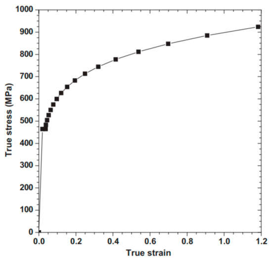
Figure 4.
True stress–strain curves of API 5L X65 steel pipe [29].

Table 2.
Mechanical property of API 5L X65 steel pipe.
The failure criterion was based on true ultimate tensile strength (UTS) of API 5L X65. [12,30]. When the von Mises stress at the corrosion defect region reaches the ultimate tensile strength (across the entire wall thickness), the steel pipe has undergone plastic collapse. If the failure criterion is reached, the internal pressure applied at the timestep is the failure pressure.
2.2. Finite Element Method Validation
Full-scale burst test results by Kim et al. [31] were used for validation of the FEM. The burst test was conducted on an API 5L X65 pipe with a single corrosion defect subjected to internal pressure only. The pipe had an outer diameter of 762 mm, a wall thickness of 17.5 mm and a pipe length of 2.3 m, enclosed with end caps. To ensure proper boundary conditions and correct application of longitudinal compressive stress, the FEM was also validated based on a full-scale burst test by Bjørnøy et al. [32]. Bjørnøy et al.’s burst tests were conducted on API 5L X52 steel pipes with an outer diameter of 324 mm, a wall thickness of 10.3 mm and a pipe length of 1.0 m. The pipe had a single corrosion defect and was subjected to internal pressure and longitudinal compressive stress. The results of the validation are tabulated in Table 3. The difference in failure pressure predicted in FEA and failure pressure from burst tests was less than 5%. As such, the FEM accurately determined the failure pressure of a corroded pipeline subjected to combined loads of internal pressure and longitudinal compressive stress.

Table 3.
Failure pressure from burst tests compared with failure pressure predicted in FEA.
2.3. Machine Learning and Artificial Neural Network
Computer-programmed learning algorithms can learn to make predictions based on information they were trained with. This method is commonly referred to as machine learning (ML). An ML technique such as artificial neural networks (ANNs) can be used to solve regression problems. An ANN can be used to correlate the non-linear relationship between corrosion parameters and the failure pressure of a pipe. For supervised learning, the dataset is labelled for training and the corrosion parameters are labelled with the target failure pressure. The dataset was obtained from FEA of an API 5L X65 pipeline with interacting corrosion defects. A supervised learning algorithm was employed in training a feedforward neural network (FFNN). To prevent overtraining, the architecture of the neural network was pruned through trial and error to improve the prediction accuracy. Hyperparameters such as the number of hidden layers and the number of hidden neurons were adjusted according to the error between the target failure pressure and the predicted target failure pressure (MSE < 1 × 10⁻⁵). The ANN framework is illustrated in a flowchart in Figure 5.
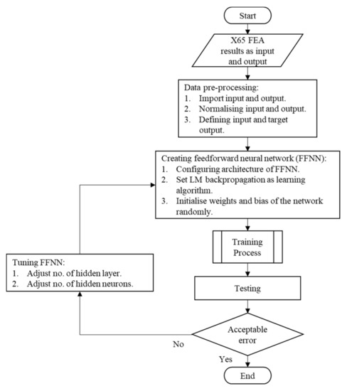
Figure 5.
ANN framework.
The Levenberg–Marquardt backpropagation (LMBP) algorithm was used to train the neural network. The algorithm performs more efficiently when compared with other learning algorithms, as LMBP uses a second-order convergence rate, which requires less time and epochs for convergence [33]. The training process of the neural network is illustrated in Figure 6. The inputs of FFNN were propagated forward through weights and biases toward hidden layers and then an output layer. The performance of the neural network was calculated by a cost function, in order to measure the error between the target output and the predicted output. The LMBP then backpropagated to update the weights and biases to minimise the cost function.
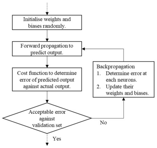
Figure 6.
Training process of the artificial neural network.
While the optimum numbers of hidden layers and hidden neurons are generally determined through trial and error, as the architecture of the neural network is heavily dependent on the size and shape (number of features and labels) of the database it is trained with, Equation (5) was used to determine the number of hidden neurons [34]:
where Nh is the number of hidden neurons and p is the number of features of the neural network. This equation was used as a reference to prune the hyperparameters, together with a trial-and-error method.
The performance of the trained ANN was evaluated through three measurements: coefficient of determination (R2), mean squared error (MSE) and mean absolute error (MAE).
where and are the actual and predicted output values for the ith output, respectively. and are the average of the actual and predicted outputs, and N is the number of samples. R2, or the squared correlation coefficient, is the evaluation of the goodness of fit for the predicted value against the actual value, where an R2 value of 1.00 corresponds to a perfect fit. The MSE is the sum of squared differences between the predictions and actual values. The MAE is the average absolute error between predictions and actual values, which measures the accuracy for the predictions.
3. Results and Discussion
3.1. Preliminary Finite Element Analysis
A preliminary study was conducted to investigate the effects of corrosion defects and load parameters on the failure pressure of a corroded API 5L X65 pipe. The parameters and their range for formulation of an equation to predict the failure pressure were subsequently determined. A corroded pipe with single and longitudinally interacting corrosion defects was studied to determine the effect of corrosion defect depth, length, width and spacing and the effect of longitudinal compressive stress on the failure pressure of the pipe. Prior literature studies considered the effect of corrosion defects subjected to internal pressure only [35,36]. The FEAs for corroded API 5L X65 pipes with a single corrosion defect were designated with the prefix SDOFAT, while the FEAs for corroded pipes with longitudinally interacting corrosion defects were designated with the prefix LIDOFAT. The results of the preliminary FEA were tabulated and compared with the failure pressure prediction by DNV’s method in Table 4. The results are expressed as the normalised failure pressure which is the ratio of the estimated failure pressure to the theoretical failure pressure of the pristine pipe, . The theoretical failure pressure of the pristine pipe is 44.93 MPa, calculated with the hoop stress equation based on the true UTS failure criterion, expressed in Equation (9):
where is the true UTS of API 5L X65, t is the thickness of the pipe and is the radius of the inner pipe.

Table 4.
FEA on a corroded pipeline with single and longitudinally interacting corrosion defects subjected to internal pressure and longitudinal compressive stress with various defect parameters.
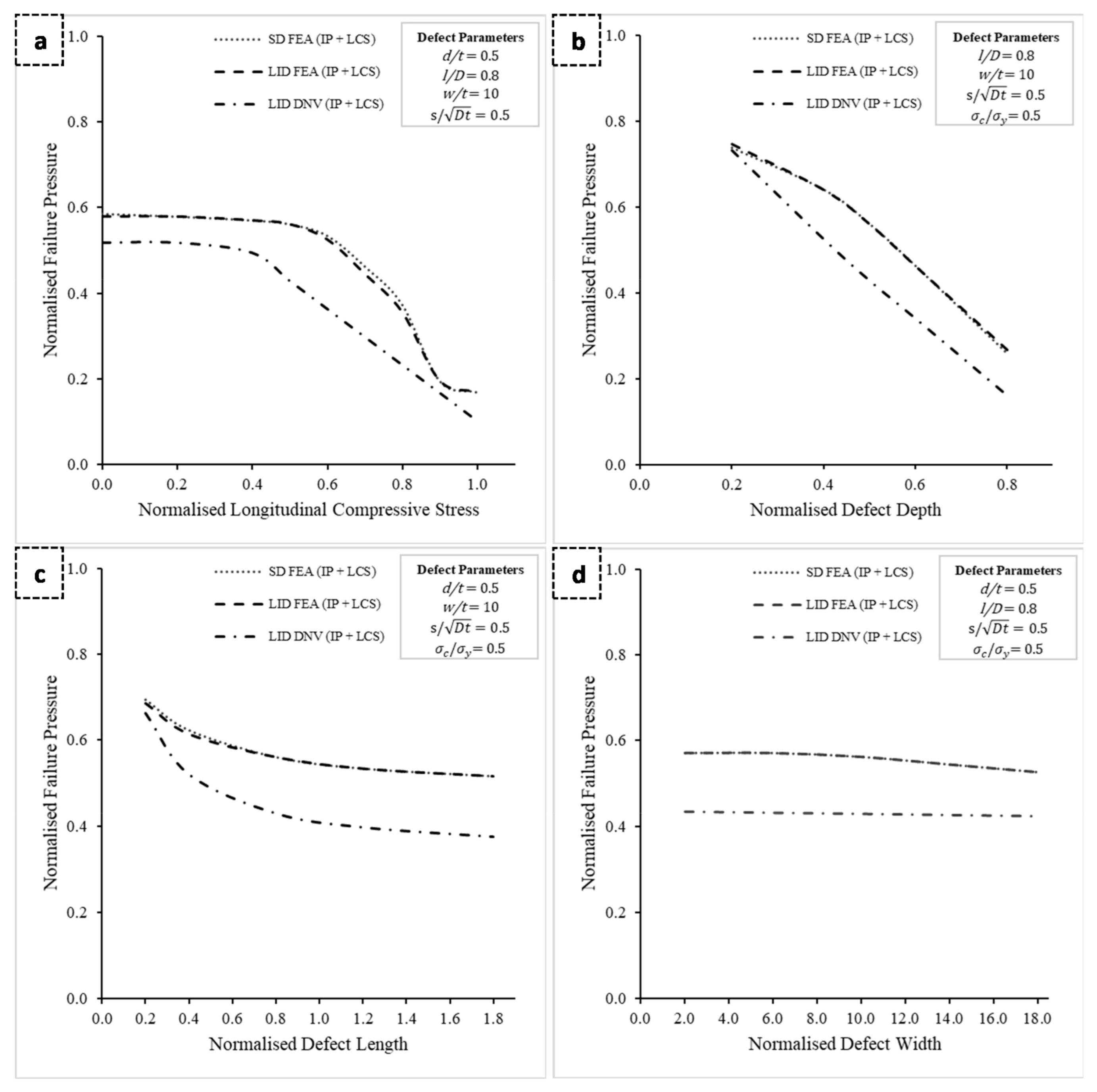
The preliminary FEA results are presented in Figure 7, where the various parameters and the corresponding failure pressure of a corroded pipeline are plotted and the differences between the predictions made by FEA and DNV for a corroded pipeline with longitudinally interacting corrosion defects (LIDs) are compared. The trends from FEA on a pipeline with a single corrosion defect (SD) were included as a control. The effect of combined loads of internal pressure (IP) and longitudinal compressive stress (LCS) on the failure pressure of a pipeline with corrosion is shown in Figure 7a. The FEA trends show a minor effect of longitudinal compressive stress on the failure pressure of pipelines with an SD and LID when the load was less than 0.4 . Longitudinal compressive stress beyond 0.4 has an adverse effect on the failure of corroded pipelines, with the failure pressure reducing exponentially for SD and LID FEA trends and linearly for the LID DNV trend. Figure 7b shows the trends for various defect depths on the failure pressure when subjected to combined loads of IP and LCS. The plot shows that the failure pressure decreases linearly when the defect depth increases. The ability of the pipeline to resist hoop stress was reduced, as the pipe wall was thinned due to corrosion [2,37,38]. The effect of the defect length on the failure pressure of a corroded pipeline is presented in Figure 7c. The failure pressure dropped with increasing corrosion defect length up to 1.2 l/D. Beyond this, the failure pressure remained relatively the same, even though the defect extended in length. This result is consistent with the previous literature for a corroded pipeline with load configurations of internal pressure only and combined loads [35,37]. The effect of the defect width on the failure pressure of a corroded pipeline is negligible, as shown in Figure 7d. The LID DNV trendline suggests that the failure pressure of a corroded pipeline remains the same regardless of the defect width. Both SD and LID FEA trendlines showed a slight decrease in failure pressure when the defect width increased, with a difference of 7.81% in the normalised failure pressure for defect widths of 2.0 and 18.0 w/t.
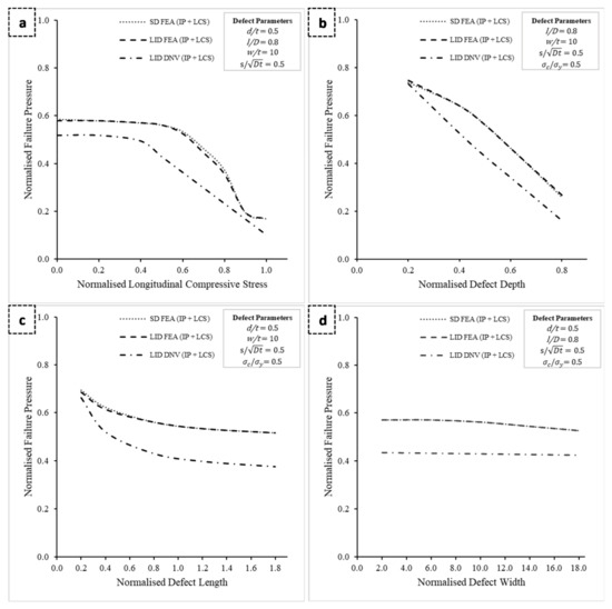
Figure 7.
FEA and DNV predictions of normalised failure pressure predictions versus normalised corrosion defect parameters and load applied: (a) normalised failure pressure versus normalised longitudinal compressive stress, (b) normalised failure pressure versus normalised defect depth, (c) normalised failure pressure versus normalised defect length, (d) normalised failure pressure versus normalised defect width.
For all the plots in Figure 7, the LID DNV trend shows the conservatism of the DNV method for estimating the failure pressure of a corroded pipeline. The DNV method predicted a lower failure pressure when compared with FEA trendlines of SD and LID. The mean average percentage difference between the failure pressure from LID FEA and LID DNV is −23.34% in Figure 7a, −21.82% in Figure 7b, −19.05% in Figure 7c and −22.44% in Figure 7d. The DNV method generally underestimated the failure pressure by 20% when compared with the more accurate FEA predictions.
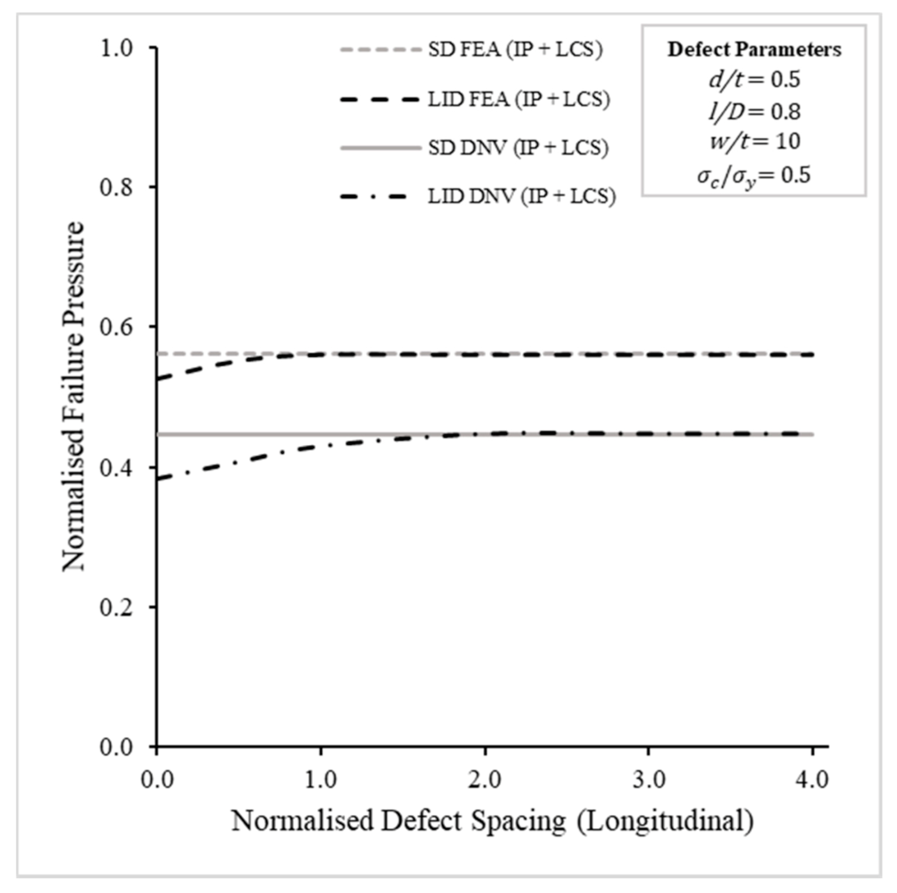
In most of the plots of Figure 7, the SD FEA trendlines were slightly above the LID FEA trendlines, which shows that an LID has a minimal effect on the failure pressure when compared with an SD. The effect of LIDs becomes evident in Figure 8, with the failure pressure affected the most when the defects were spaced closely together. As the spacing between the defects increased in the longitudinal direction, the failure pressure increased up to the failure pressure of single-defect corrosion. The trend was visible in both FEA and DNV trendlines, where the spacing was sufficiently far apart and the interaction between the defects became negligible. Defects spaced beyond the interaction limit act as single corrosion defects, with the failure pressure determined by the most severe corrosion defect [5]. From the FEA trendline, the interaction limit is at 1.0 , while the interaction limit is 2.0 for the DNV trendline.
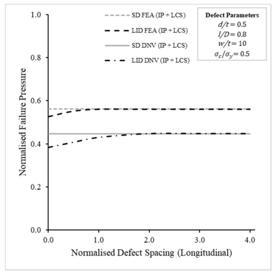
Figure 8.
FEA and DNV predictions of normalised failure pressure predictions versus normalised longitudinal defect spacing.
3.2. Further Finite Element Analysis
The preliminary FEA provided insights to select the appropriate parametric bound for the formulation of an equation to predict the failure pressure for a pipeline with longitudinal interacting corrosion defects. The significance of the effect of the corrosion defect geometry and longitudinal compressive stress was ranked according to their trendline gradient in Figure 7, where their influence on the failure pressure of the pipeline was plotted. The corrosion defect depth has the most significance, with an average gradient of −0.81 in Figure 7a, followed by longitudinal compressive stress with an average gradient of −0.43, the corrosion defect length with an average gradient of −0.097, the corrosion defect spacing with an average gradient of 0.0062 and the corrosion defect width with an average gradient of −0.0029. Only significant parameters and their limits were considered for further FEA, as limits where the failure pressure starts to plateau were redundant. The appropriate limits of the corrosion defect depth are 0.2 and 0.8 d/t and 0.2 and 0.7 for longitudinal compressive stress. Loads beyond these upper limits risk buckling failure. Defect lengths from 0.2 to 1.2 l/D influence the failure pressure, and beyond this range, the failure pressure plateaus. Defect spacing from 0 to 3.0 was selected, while the defect width has a negligible influence on the failure pressure of corroded pipelines; therefore, the parameter was excluded in further FEA. The parameters selected were investigated in full factorial and the results of further FEA were tabulated in Table 5, Table 6, Table 7, Table 8, Table 9 and Table 10.

Table 5.
FEA on corroded pipeline with longitudinally interacting corrosion defect (LID) subjected to internal pressure and 0 longitudinal compressive stress.

Table 6.
FEA on corroded pipeline with LID subjected to internal pressure and 0.2 longitudinal compressive stress.

Table 7.
FEA on corroded pipeline with LID subjected to internal pressure and 0.4 longitudinal compressive stress.

Table 8.
FEA on corroded pipeline with LID subjected to internal pressure and 0.5 longitudinal compressive stress.

Table 9.
FEA on corroded pipeline with LID subjected to internal pressure and 0.6 longitudinal compressive stress.

Table 10.
FEA on corroded pipeline with LID subjected to internal pressure and 0.7 longitudinal compressive stress.
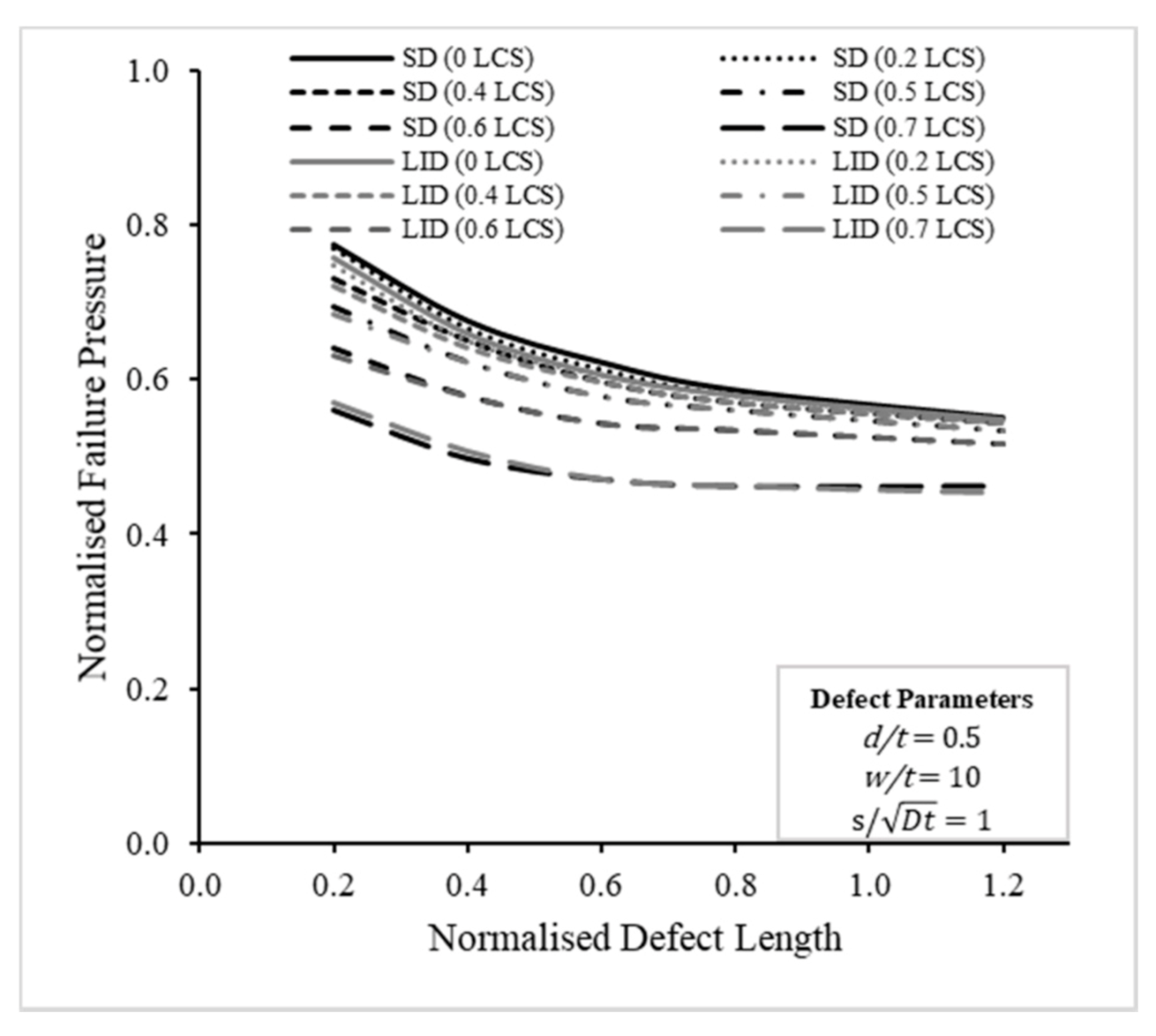
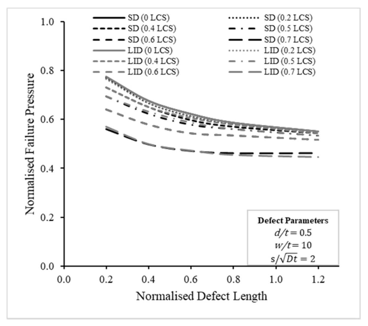
A full factorial design to investigate the relationship between the corrosion defect parameters and load was performed and gave insightful results on the interaction limit of the longitudinal interacting corrosion defects. When the spacing between interacting corrosion defects was within the interaction limit, the failure pressure was lower than single corrosion defects, as shown in Figure 9, Figure 10 and Figure 11. The failure pressures of LIDs and SDs with defect lengths for all longitudinal compressive stresses were considered for different defect spacings, where Figure 9 shows the failure pressure at a defect spacing of 0.5, Figure 10 shows the failure pressure at a defect spacing of 1.0 and Figure 11 shows the failure pressure at a defect spacing of 2.0. When the defects were close to each other (defect spacing of 0.5 in Figure 9), the failure pressures of most LID trendlines were lower than the failure pressures for SD trendlines. As the spacing increased between the defects, the failure pressure of most LID trendlines increased, approaching the failure pressure of SD trendlines, as seen in Figure 10. When the LID defect spacings were sufficiently far apart, the failure pressures were the same as the failure pressures of SD trendlines, as seen in Figure 11. The interaction limit for the API 5L X65 pipeline with longitudinal interacting defects is therefore 2.0 , consistent with DNV.
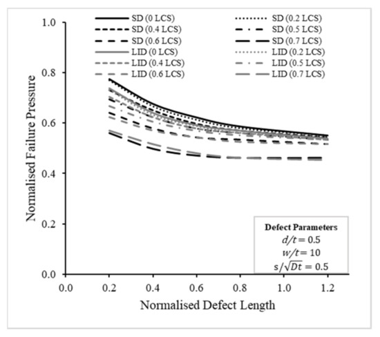
Figure 9.
Single corrosion defect (SD) and LID comparison of normalised failure pressure predictions versus normalised longitudinal defect spacing across different longitudinal compressive stresses for defect spacing of 0.5.

Figure 10.
SD and LID comparison of normalised failure pressure predictions versus normalised longitudinal defect spacing across different longitudinal compressive stresses for defect spacing of 1.

Figure 11.
SD and LID comparison of normalised failure pressure predictions versus normalised longitudinal defect spacing across different longitudinal compressive stresses for defect spacing of 2.
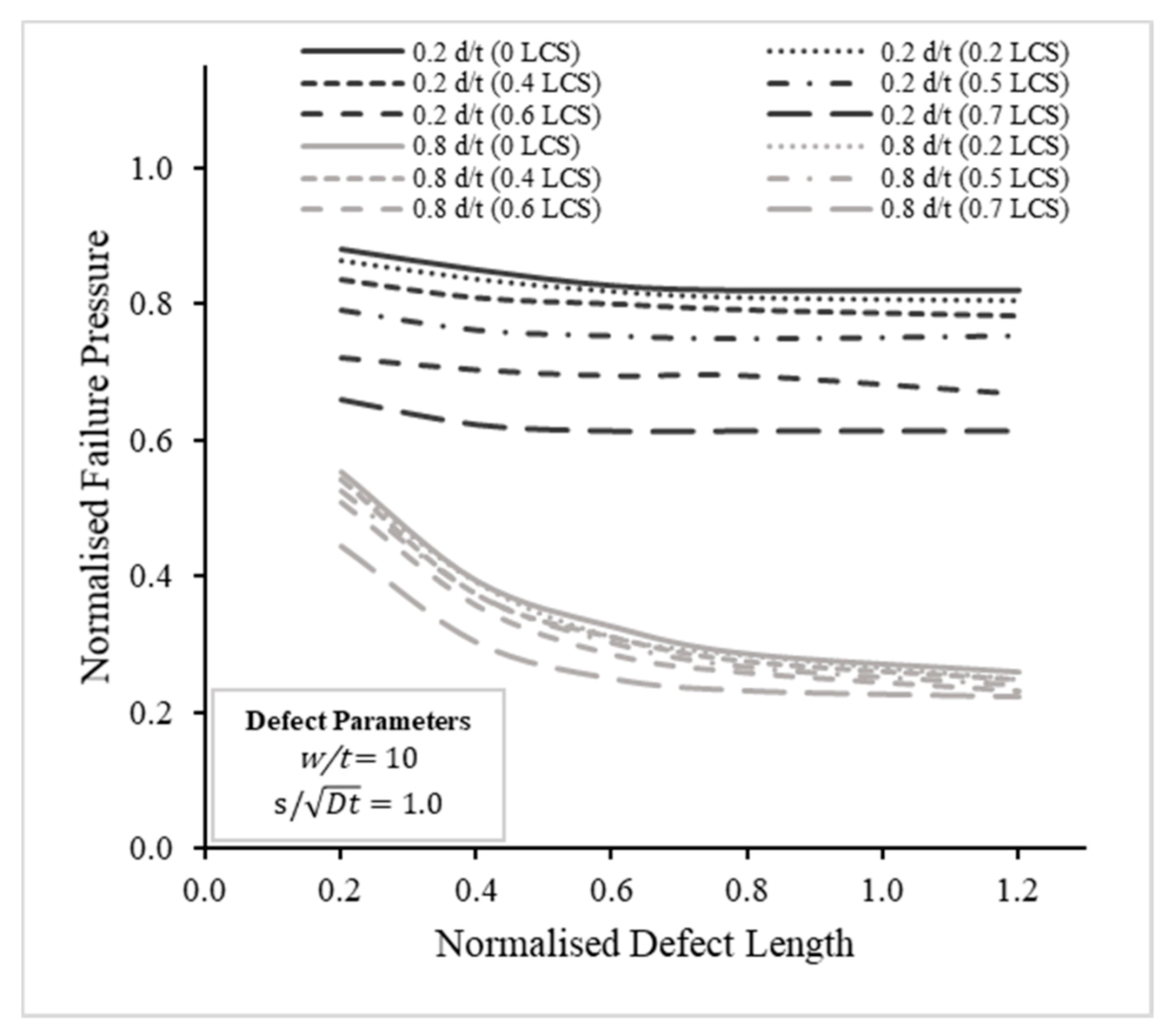
The full factorial FEA also highlighted the detrimental effect of the corrosion defect depth when a corroded pipeline with LIDs was subjected to a combined load of internal pressure and longitudinal compressive stress. In Figure 12, the failure pressures of a pipeline with shallow (0.2 d/t) and deep (0.8 d/t) defect depths are plotted against defect depths for various longitudinal compressive stresses. From the figure, increasing defect depth causes the failure pressure to increase significantly when the defect length increases. The gradients of both defect depths’ trendlines remained relatively unchanged for various longitudinal compressive stresses, with the trendline gradients for the deep defect being greater than those for the shallow defect. The gradients show that the defect depth has a greater effect on the failure pressure.
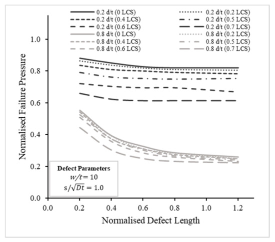
Figure 12.
Comparison of normalised failure pressure predictions versus normalised longitudinal defect spacing across different longitudinal compressive stresses for defect depths of 0.2 and 0.8.
3.3. Development of New Assessment Equation Using ANN
The ANN model was developed with MathWorks MATLAB R2019b. The architecture of the ANN model was based on the feedforward neural network (FFNN) with the Levenberg–Marquardt backpropagation (LMBP) learning algorithm. The network structure visualised in MATLAB is shown in Figure 13. Corrosion defect depth d/t, corrosion defect length l/D, corrosion defect spacing and axial compressive stress were used as inputs for the ANN model and the target output was the failure pressure . The inputs and output were normalised to be between the range of −1 and 1 using Equation (10), so that they were within the data range that the sigmoid activation functions lie in.
where is the normalisation value ranging from −1 to 1 and is the de-normalisation value, which ranges according to its dataset.

Figure 13.
Architecture of the ANN model as represented in MATLAB.
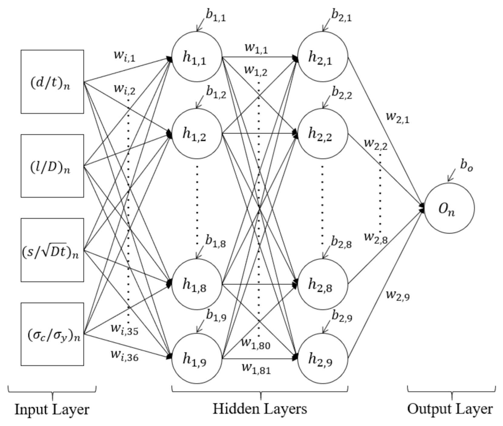
The database for training was based on the full factorial design of the FEA results. The best performing neural network configuration was determined through trial and error. After numerous prunings, the network with two hidden layers with five hidden neurons in each hidden layer was finalised. Hyperbolic tangent sigmoid transfer functions were utilised in the hidden layers, while a linear transfer function was applied in the output layer. To formulate the failure pressure prediction equation, the trained neural network was expressed in mathematical form.
The components of the ANN model can be visualised as Figure 14, where the input, hidden and output neurons are connected through links between their layers. The links were weighted, and values passed from neurons to neurons were amplified or dampened depending on the weights of the links. denotes weights linking the input layer to hidden layer 1 . denotes weights linking to hidden layer 2 . denotes weights linking to the output layer. Biases () are constant non-zero values of hidden neurons which were then summed with the product of inputs and weights. The result was then transferred through the transfer function of the neuron as its output.

Figure 14.
Architecture of FFNN model employed.
The weights and biases of the links were constantly updated until the training stopped when the predictions from the ANN achieved the target error difference with an R2 of 0.9997, MSE of 7.067 × 10⁻⁵ and MAE of 0.0067. Weights and biases from the trained ANN model were expressed in mathematical form from Equations (11)–(13) to formulate the failure pressure prediction equation.
where is the hyperbolic tangent sigmoid transfer function,
and is the linear transfer function,
The ANN model used to develop the equation was based on the results of FEA on an API 5L X65 corroded pipeline with LIDs subjected to combined loads of internal pressure and longitudinal compressive stress. Therefore, the equations are recommended for parameters within the investigated range only.
3.4. Performance of New Assessment Equation
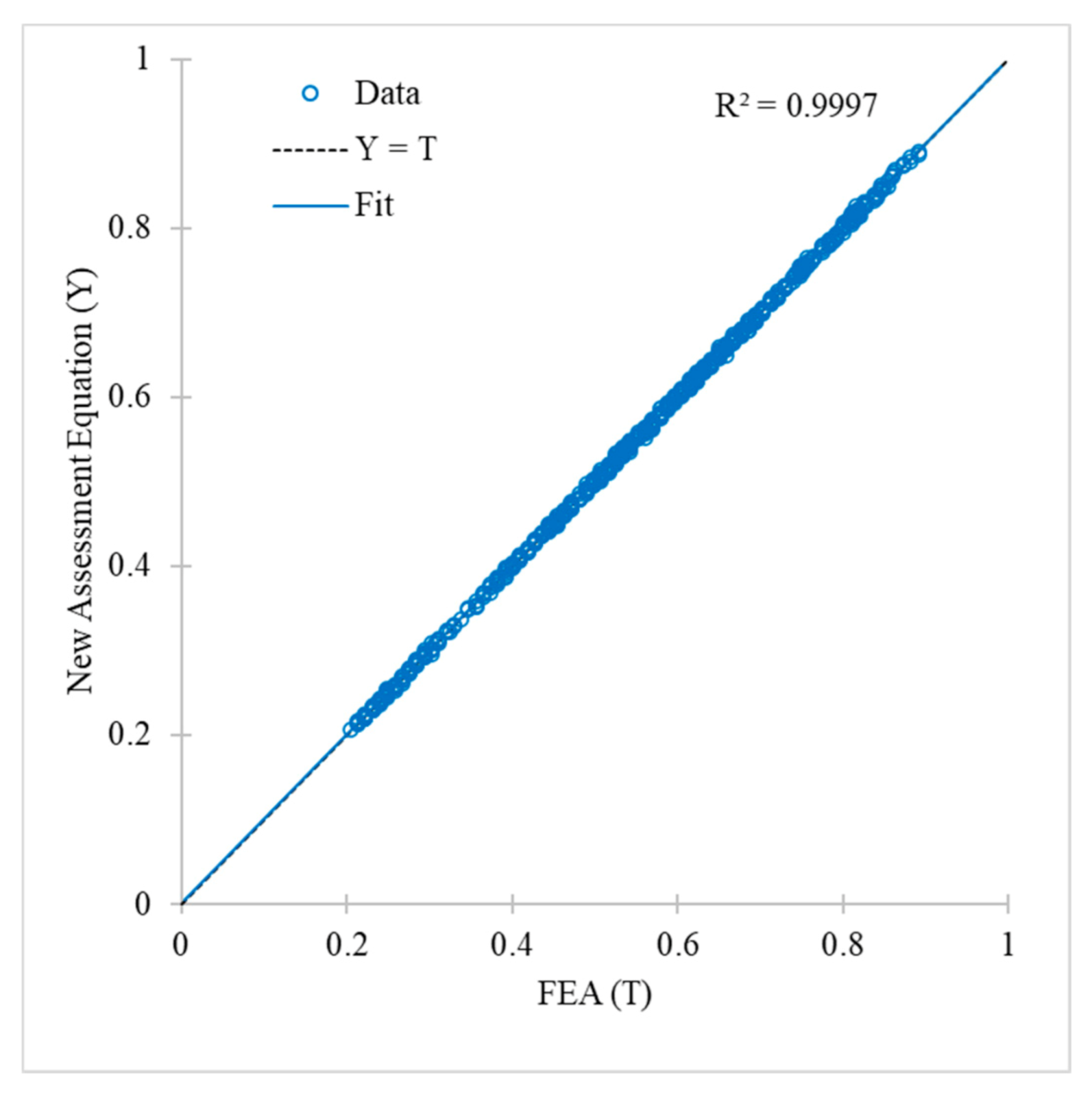
The newly developed equations were checked to ensure satisfactory performance. The predictions from the new equations were compared with results from FEA, which were the target outputs of the ANN. They were plotted as a regression plot in Figure 15. The corresponding R2 value is 0.9997, the MSE is 8.335 × 10⁻⁶ and the MAE is 2.315 × 10⁻³. The percentage error of the predictions from new equations ranged from −2.26% to 2.07%, with a standard deviation of 0.49.
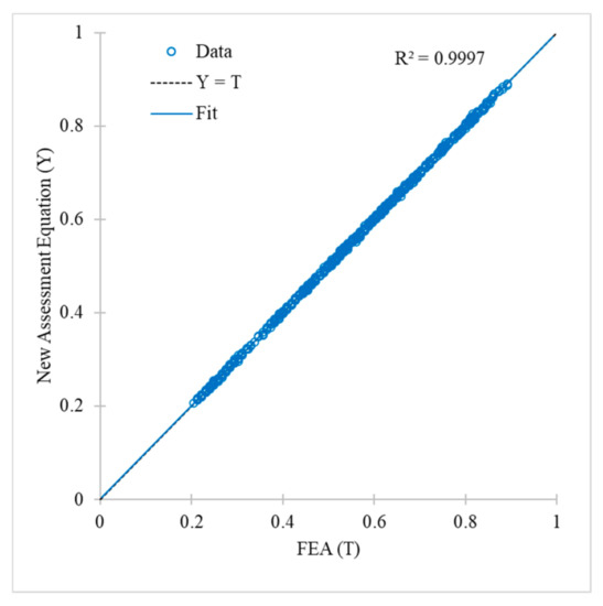
Figure 15.
Regression plot of failure pressure predictions made by the new assessment equations and FEA.
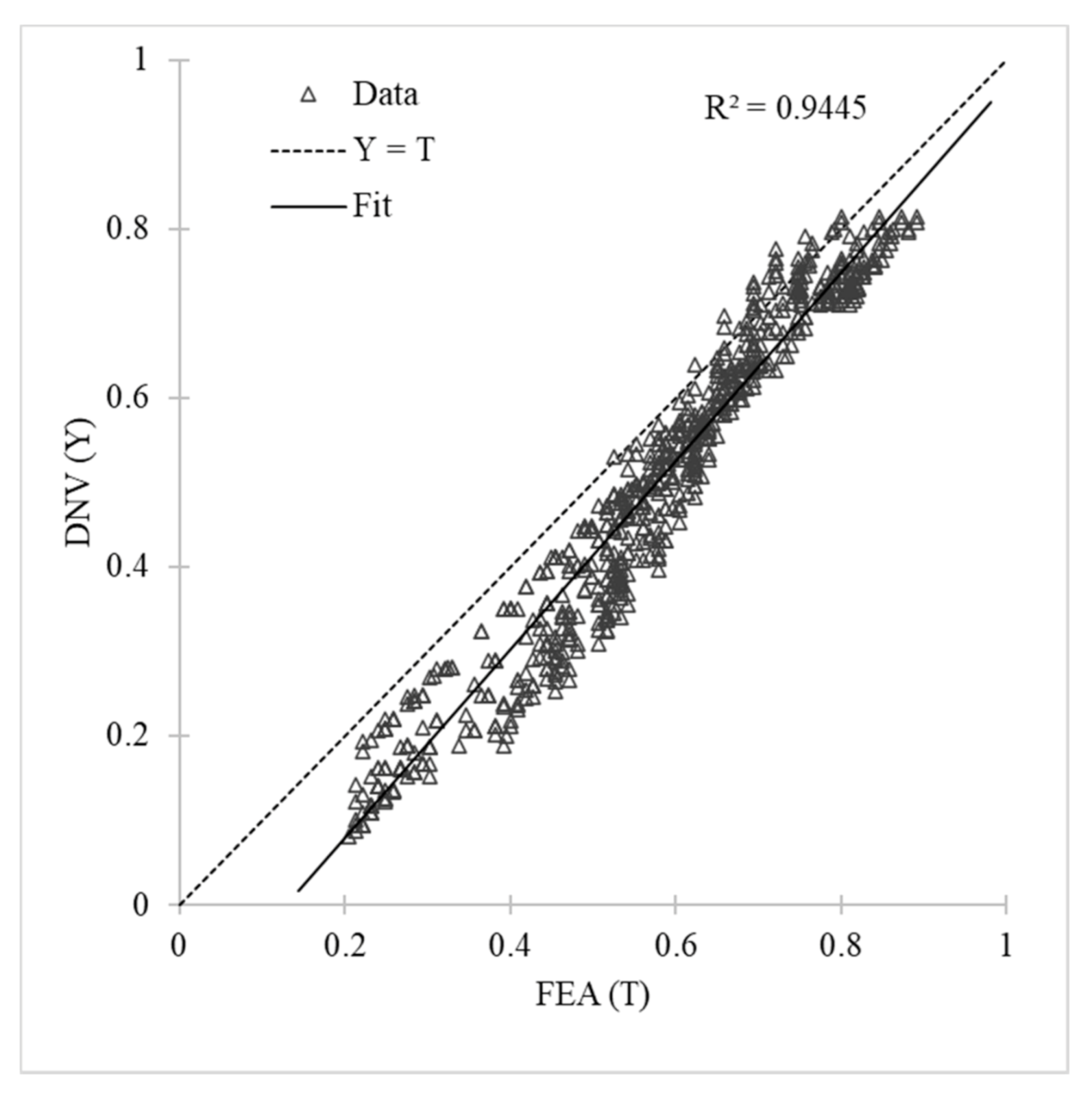
For comparison, the predictions from the DNV assessment method were compared with the results of the FEA as well, as shown in Figure 16. The R2 value for predictions made with the DNV method is 0.9445, with an MSE of 8.973 × 10⁻³ and an MAE of 8.242 × 10⁻². The conservatism of the DNV method is apparent through its lower failure pressure predictions, with the percentage error ranging from −60.13% to 7.70%, with a standard deviation of 13.90. The conservative predictions may result in premature maintenance and shutdowns.

Figure 16.
Regression plot of failure pressure predictions made using DNV method and FEA results.
The equations were tested with an unseen dataset for validation and to determine their performance. Table 11 tabulates the unseen FEA results and the predictions from the equations.

Table 11.
Failure pressure predictions using FEA and predictions made based on the equations on unseen dataset.
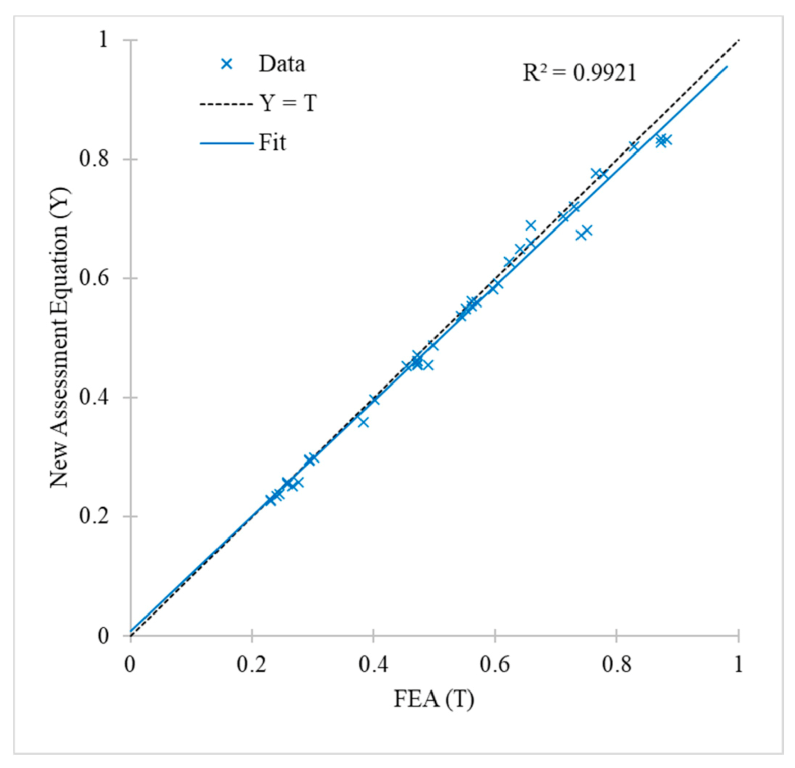
The comparison of failure pressure predictions from the equations and unseen FEA dataset are plotted as a regression plot in Figure 17. The R2 value is 0.9921, the MSE is 4.746 × 10⁻⁴ and the MAE is 1.374 × 10⁻². The percentage error of the predictions based on the equations ranges from −9.39% to 4.63%, with a standard deviation of 2.83. Based on their performance, the predictions based on the equations are within ±10% of the failure pressure predicted by FEA.
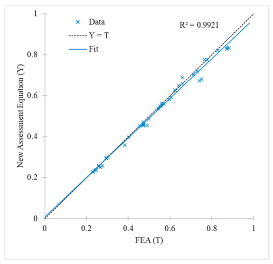
Figure 17.
Regression plot of the predicted normalised failure pressures based on the equations and FEA results from unseen dataset.
3.5. Recommendations on the Failure Pressure Prediction Equations
Predictions from an ANN depend greatly on the dataset it was trained with. Therefore, the scope and range of its predictive ability could be expanded to include more parameters such as the material’s UTS. A more robust equation could then be formulated from the trained ANN. Nonetheless, the equations formulated in this study achieved their intended goal of improving failure pressure prediction. They are comparable to the DNV assessment method using the FEM based on the material’s true UTS as the failure criterion. The equations could be used to calculate the failure pressure of corroded API 5L X65 pipelines quickly when set up correctly in a spreadsheet. However, the equations are recommended for parameters within the investigated range only. Nevertheless, all factors should be considered when assessing corroded pipelines, including the failure pressure prediction equations and established assessment method for a comprehensive pipeline integrity management.
4. Conclusions
An equation for the failure pressure prediction of a corroded pipeline subjected to combined loads was formulated from an ANN trained with a database generated by FEA. FEA was performed on an API 5L X65 grade steel pipe with longitudinal interacting corrosion defects and subjected to internal pressure and longitudinal compressive stress. The pipe was considered to have failed when the von Mises stress of its wall exceeded the true UTS in the FEA. The FEM was validated with burst tests to ensure an accurate representation of an actual pipeline failure pressure. Preliminary FEA was conducted to better understand the influence of the corrosion defect parameters and loading applied on the failure pressure of a pipe. The results from this preliminary FEA were compared with the DNV method, which revealed conservative failure pressure estimations by the DNV method. Further FEA was carried out in full factorial design for significant parameters only. Defect depth limits of 0.2 and 0.8 d/t; defect length limits of 0.2 and 1.2 l/D; defect spacing limits of 0 to 3 ; and longitudinal compressive stress limits of 0 to 0.7 were considered. In the full factorial design FEA, the interaction limit of longitudinally interacting defects was found to be 2.0 .
The results from FEA were used to train an ANN to formulate a failure pressure prediction equation. The training of the ANN was stopped when the error of its predictions achieved a satisfactory level of MSE < 1 × 10⁻⁵. The weights and biases from the trained ANN were expressed in mathematical form to formulate the failure pressure prediction equations. The failure pressure equations were compared with the DNV method and tested with an unseen FEA dataset. The predictions from the failure pressure prediction equations were accurate with an R2 value of 0.9921, an MSE of 4.746 × 10⁻⁴ and an MAE of 1.374 × 10⁻², with the percentage error ranging from −9.39% to 4.63%, with a standard deviation of 2.83. All factors should be considered when assessing the failure pressure of a corroded pipeline, and the equations should complement, rather than replace, an established assessment method for a comprehensive and rigorous pipeline assessment.
Author Contributions
Conceptualization, M.L. and S.K.; methodology, M.L. and S.K.; software, M.L.; validation, M.L.; formal analysis, M.L.; investigation, M.L. and S.K.; resources, M.L., S.K. and M.O.; data curation, M.L.; writing—original draft preparation, M.L., S.K. and M.O.; writing—review and editing, M.L., S.K. and M.O.; visualization, M.L., S.K. and M.O.; supervision, S.K. and M.O.; project administration, S.K. and M.O.; funding acquisition, S.K. and M.O. All authors have read and agreed to the published version of the manuscript.
Funding
This research was funded by Ministry of Higher Education, Malaysia (FRGS/1/2018/TK03/UTP/02/1).
Institutional Review Board Statement
Not applicable.
Informed Consent Statement
Not applicable.
Data Availability Statement
The data presented in this study are available within the article.
Conflicts of Interest
The authors declare no conflict of interest.
References
- Taylor, N.; Clubb, G.; Matheson, I. The effect of bending and axial compression on pipeline burst capacity. In Proceedings of the SPE Offshore Europe Conference & Exhibition; Society of Petroleum Engineers (SPE), Aberdeen, Scotland, UK, 8–11 September 2015; Society of Petroleum Engineers: Richardson, TX, USA, 2015. [Google Scholar]
- Han, C.J. Failure Pressure Analysis of the Pipe with Inner Corrosion Defects by FEM. Int. J. Electrochem. Sci. 2016, 11, 5046–5062. [Google Scholar] [CrossRef]
- Benjamin, A.C.; Freire, J.L.F.; Vieira, R.D.; Diniz, J.L.C.; De Andrade, E.Q. Burst tests on pipeline containing interacting corrosion defects. In Proceedings of the 24th International Conference on Offshore Mechanics and Arctic Engineering, Halkidiki, Greece, 12–17 June 2005; American Society of Mechanical Engineers: New York, NY, USA, 2005; Volume 3, pp. 403–417. [Google Scholar]
- DNV GL. Recommended Practice—Corroded Pipelines (DNVGL-RP-F101); DNV GL: Oslo, Norway, 2017. [Google Scholar]
- Silva, R.; Guerreiro, J.; Loula, A. A study of pipe interacting corrosion defects using the FEM and neural networks. Adv. Eng. Softw. 2007, 38, 868–875. [Google Scholar] [CrossRef]
- ASME. Manual for Determining the Remaining Strength of Corroded Pipelines: B31G; American Society of Mechanical Engineers: New York, NY, USA, 2012. [Google Scholar]
- Kiefner, J.F.; Vieth, P.H. New Method Corrects Criterion for Evaluating Corroded Pipe. Oil Gas J. 1990, 88, 56–59. [Google Scholar]
- Amandi, K.; Diemuodeke, E.; Briggs, T.; Pham, D. Model for remaining strength estimation of a corroded pipeline with interacting defects for oil and gas operations. Cogent Eng. 2019, 6, 1663682. [Google Scholar] [CrossRef]
- Khalajestani, M.K.; Bahaari, M.R.; Salehi, A.; Shahbazi, S. Predicting the limit pressure capacity of pipe elbows containing single defects. Appl. Ocean Res. 2015, 53, 15–22. [Google Scholar] [CrossRef]
- Khalajestani, M.K.; Bahaari, M.R. Investigation of pressurized elbows containing interacting corrosion defects. Int. J. Press. Vessel. Pip. 2014, 123–124, 77–85. [Google Scholar] [CrossRef]
- Chen, Y.; Zhang, H.; Zhang, J.; Li, X.; Zhou, J. Failure analysis of high strength pipeline with single and multiple corrosions. Mater. Des. 2015, 67, 552–557. [Google Scholar] [CrossRef]
- Arumugam, T.; Karuppanan, S.; Ovinis, M. Finite element analyses of corroded pipeline with single defect subjected to internal pressure and axial compressive stress. Mar. Struct. 2020, 72, 102746. [Google Scholar] [CrossRef]
- Wang, N.; Zarghamee, M.S. Evaluating Fitness-for-Service of Corroded Metal Pipelines: Structural Reliability Bases. J. Pipeline Syst. Eng. Pract. 2014, 5, 04013012. [Google Scholar] [CrossRef]
- Liu, H.; Khan, F.; Thodi, P. Revised burst model for pipeline integrity assessment. Eng. Fail. Anal. 2017, 80, 24–38. [Google Scholar] [CrossRef]
- Shuai, Y.; Shuai, J.; Xu, K. Probabilistic analysis of corroded pipelines based on a new failure pressure model. Eng. Fail. Anal. 2017, 81, 216–233. [Google Scholar] [CrossRef]
- Motta, R.S.; Cabral, H.L.; Afonso, S.M.; Willmersdorf, R.B.; Bouchonneau, N.; Lyra, P.R.; De Andrade, E.Q. Comparative studies for failure pressure prediction of corroded pipelines. Eng. Fail. Anal. 2017, 81, 178–192. [Google Scholar] [CrossRef]
- Bruère, V.M.; Bouchonneau, N.; Motta, R.S.; Afonso, S.M.B.; Willmersdorf, R.B.; Lyra, P.R.M.; Torres, J.V.S.; De Andrade, E.Q.; Cunha, D.J.S. Failure pressure prediction of corroded pipes under combined internal pressure and axial compressive force. J. Braz. Soc. Mech. Sci. Eng. 2019, 41, 172. [Google Scholar] [CrossRef]
- Belachew, C.T.; Ismail, M.C.; Karuppanan, S. Burst Strength Analysis of Corroded Pipelines by Finite Element Method. J. Appl. Sci. 2011, 11, 1845–1850. [Google Scholar] [CrossRef][Green Version]
- Smith, M.Q.; Grigory, S.C. New Procedures for the Residual Strength Assessment of Corroded Pipe Subjected to Combined Loads. In Proceedings of the International Pipeline Conference, IPC, Calgary, AB, Canada, 9–13 June 1996; American Society of Mechanical Engineers Digital Collection: New York, NY, USA, 1996; pp. 387–400. [Google Scholar] [CrossRef]
- Roy, S.; Grigory, S.; Smith, M.; Kanninen, M.F.; Anderson, M. Numerical Simulations of Full-Scale Corroded Pipe Tests with Combined Loading. J. Press. Vessel. Technol. 1997, 119, 457–466. [Google Scholar] [CrossRef]
- Mohd, M.H.; Lee, B.J.; Cui, Y.; Paik, J.K. Residual strength of corroded subsea pipelines subject to combined internal pressure and bending moment. Ships Offshore Struct. 2015, 10, 1–11. [Google Scholar] [CrossRef]
- Keshtegar, B.; Miri, M. Reliability analysis of corroded pipes using conjugate HL–RF algorithm based on average shear stress yield criterion. Eng. Fail. Anal. 2014, 46, 104–117. [Google Scholar] [CrossRef]
- Keshtegar, B.; Seghier, M.E.A.B. Modified response surface method basis harmony search to predict the burst pressure of corroded pipelines. Eng. Fail. Anal. 2018, 89, 177–199. [Google Scholar] [CrossRef]
- Seghier, M.E.A.B.; Keshtegar, B.; Elahmoune, B. Reliability analysis of low, mid and high-grade strength corroded pipes based on plastic flow theory using adaptive nonlinear conjugate map. Eng. Fail. Anal. 2018, 90, 245–261. [Google Scholar] [CrossRef]
- Han, L.; Han, L.; Liu, C. Neural network applied to prediction of the failure stress for a pressurized cylinder containing defects. Int. J. Press. Vessel. Pip. 1999, 76, 215–219. [Google Scholar] [CrossRef]
- Tohidi, S.; Sharifi, Y. Load-carrying capacity of locally corroded steel plate girder ends using artificial neural network. Thin-Walled Struct. 2016, 100, 48–61. [Google Scholar] [CrossRef]
- British Standard. Guide to methods for assessing the acceptability of flaws in metallic structures. In BS 7910:2013; British Standard Institute: London, UK, 2013. [Google Scholar]
- Kim, Y.-J.; Oh, C.-S. Limit loads for pipe bends under combined pressure and in-plane bending based on finite element limit analysis. Int. J. Press. Vessel. Pip. 2006, 83, 148–153. [Google Scholar] [CrossRef]
- Baek, J.-H.; Kim, Y.-P.; Kim, W.-S.; Koo, J.-M.; Seok, C.-S. Load bearing capacity of API X65 pipe with dent defect under internal pressure and in-plane bending. Mater. Sci. Eng. A 2012, 540, 70–82. [Google Scholar] [CrossRef]
- Xu, W.-Z.; Li, C.B.; Choung, J.; Lee, J.-M. Corroded pipeline failure analysis using artificial neural network scheme. Adv. Eng. Softw. 2017, 112, 255–266. [Google Scholar] [CrossRef]
- Kim, Y.-P.; Kim, W.-S.; Lee, Y.-K.; Oh, K.-H. The Evaluation of Failure Pressure for Corrosion Defects within Girth or Seam Weld in Transmission Pipelines. In Proceedings of the 2004 International Pipeline Conference, Calgary, AB, Canada, 4–8 October 2004; ASMEDC: New York, NY, USA, 2004; Volume 1–3, pp. 1847–1855. [Google Scholar]
- Bjørnøy, O.H.; Sigurdsson, G.; Cramer, E. Residual Strength of Corroded Pipelines, DNV Test Results. In Proceedings of The Tenth International Offshore and Polar Engineering Conference, Seattle, WA, USA, 28 May–2 June 2000; International Society of Offshore and Polar Engineers: Mountain View, CA, USA, 2000. [Google Scholar]
- Hagan, M.; Menhaj, M. Training feedforward networks with the Marquardt algorithm. IEEE Trans. Neural Netw. 1994, 5, 989–993. [Google Scholar] [CrossRef]
- Panchal, F.S.; Panchal, M. Review on Methods of Selecting Number of Hidden Nodes in Artificial Neural Network. Int. J. Comput. Sci. Mob. Comput. 2014, 3, 455–464. [Google Scholar]
- Cosham, A.; Hopkins, P.; Macdonald, K. Best practice for the assessment of defects in pipelines—Corrosion. Eng. Fail. Anal. 2007, 14, 1245–1265. [Google Scholar] [CrossRef]
- Su, C.-L.; Li, X.; Zhou, J. Failure pressure analysis of corroded moderate-to-high strength pipelines. China Ocean Eng. 2016, 30, 69–82. [Google Scholar] [CrossRef]
- Ahammed, M.; Melchers, R. Reliability estimation of pressurised pipelines subject to localised corrosion defects. Int. J. Press. Vessel. Pip. 1996, 69, 267–272. [Google Scholar] [CrossRef]
- Oh, C.-K.; Kim, Y.-J.; Park, C.-Y. Effects of local wall thinning on net-section limit loads for pipes under combined pressure and bending. Nucl. Eng. Des. 2009, 239, 261–273. [Google Scholar] [CrossRef]
Publisher’s Note: MDPI stays neutral with regard to jurisdictional claims in published maps and institutional affiliations. |
© 2021 by the authors. Licensee MDPI, Basel, Switzerland. This article is an open access article distributed under the terms and conditions of the Creative Commons Attribution (CC BY) license (http://creativecommons.org/licenses/by/4.0/).

