How Good Is the STW Sensor? An Account from a Larger Shipping Company

Abstract

This paper examines the statistical properties and the quality of the speed through water (STW) measurement based on data extracted from almost 200 container ships of Maersk Line’s fleet for 3 years of operation. The analysis uses high-frequency sensor data along with additional data sources derived from external providers. The interest of the study has its background in the accuracy of STW measurement as the most important parameter in the assessment of a ship’s performance analysis. The paper contains a thorough analysis of the measurements assumed to be related with the STW error, along with a descriptive decomposition of the main variables by sea region including sea state, vessel class, vessel IMO number and manufacturer of the speed-log installed in each ship. The paper suggests a semi-empirical method using a threshold to identify potential error in a ship’s STW measurement. The study revealed that the sea region is the most influential factor for the STW accuracy and that $26\%$ of the ships of the dataset’s fleet warrant further investigation.

1. Introduction

1.1. Background

The shipping industry has a strong wish to reduce the environmental effects of their operations and become sustainable. In addition to this, strict regulations on notably carbon emissions make it necessary for shipping companies to closely monitor and evaluate the performance of both the single ship and the entire fleet daily. Increasing use of on-board sensors and improved speed-power performance models have led to a significant increase in the fuel efficiency. The central parameter in this context is the measured speed with which a ship advances. Thus, the necessary power to achieve a given speed is approximately proportional to the speed cubed [1,2,3]. Consequently, it is clear that any uncertainty or error in the measured speed can have a detrimental effect on the outcome of speed-power performance models.

At sea, the speed of an advancing ship is measured either relative to the seabed (speed over ground—SOG) or relative to the surrounding water flowing past the hull (speed through water—STW). Both speed types apply in modern navigation systems [4]. However, for all models addressing problems related to speed-power performance, STW is the measurement that enters the models; obviously noting that the two measurements (STW and SOG) are related through the speed of sea current. Typically, maritime speed logging devices use one of the following measurement principles to obtain the STW: water pressure, electromagnetic induction, or the transmission of low frequency radio waves [5]. The latter refers to as the Doppler velocity log (DVL), which is the speed-log used by the ships dealt with in this paper, and used by the majority of today’s merchant ships.

DVLs are installed along the centerline of the hull at a dry accessible location in the bow of the ship, where the flow is as undisturbed as possible and contains few air bubbles. It is evident that DVL sensors measure in a highly fluctuating environment [6]. The flow around a ship is affected by eddies, currents, waves, stratified current layers etc. Furthermore, the sensor itself moves relative to the water due to ship motions [7]. Accurate measurement of ship speed is therefore difficult, notwithstanding STW is the most important parameter for performance analysis. The calculation of the STW accuracy has been a challenging task for the experts of the shipping industry ever since the launch of the first DVL sensor used for underwater navigation [7,8,9,10,11,12,13,14,15,16,17].

Seafarers, marine engineers, and land-based performance analysts recognize that there is error involved in the STW measurement greater than the values indicated by the respective DVL manufacturers. Likewise, there are claims of observed constant offset in the STW measurements [18]. Reported examples from daily operations include also sudden jumps and drifts in the STW signal with measurements constantly decreasing/increasing for relatively long periods (hours), despite a maintained constant speed as secured by crew. Such incidents, apart from bringing mistrust to the crew navigating the ship, they also shift the outcome of any dynamic voyage planning and they finally cause headaches to performance analysts. However, the above-mentioned testimonies will remain unsupported if they are not properly investigated and documented. Individual cases are not enough to hold assumptions and generalize for a larger extent.

1.2. Objective and Scientific Contribution of Study

Although all the above-mentioned studies enhanced the literature of Doppler logging devices, there has never been an attempt to quantify the deriving error using real sensor data from a large fleet consisting of ships with different characteristics. This paper constitutes an initial attempt to quantify the error affecting the STW measurement using high-frequency data from approximately 200 container ships sailing for 3 years. As such, it is an account from a large container shipping company with the aim to make a systematic analysis of different sets of operational and environmental data collected and stored in-company and obtained from third parties. The overall objective of the paper is to contribute towards a better understanding of the responsible causes suspect to degrade the STW measurement.

1.3. Problem Formulation

Understanding a ship’s SOG and STW accurately joins with a range of daily operational challenges on-board the ships and on-shore for any shipping company. One of the main objectives of most shipping companies is to model the current performance of their ships and forecast what will happen in the very near or distant future. For instance, looking at the short-term voyage planning model which provides advice for the crew, an internal company study indicates that the average speed prediction profile to arrive on time in all operational conditions should be less than $1.0$ kn RMSE (Root Mean Square Error) for the crew to trust the advice. This leads to several interesting research questions, like:

• What parameters and external conditions seem to be the most influential on the STW measurements accuracy?
• How often and where are these parameters and conditions observed?
• Assuming a given advice quality requirement (threshold), how sensitive are the answers to the above questions?

In this study, three speed signals have been used for the purpose of answering these questions. The first is the STW, referred to by $U_w$, the second is the SOG, given as $U_g$, and the third is the speed of the surface currents projected on the ship’s true heading, defined by $U_c$. Those three signals have a theoretical relationship which constitutes the foundations of this study.

$$\begin{array}{c}\hfill U_w^b=U_g^b-U_c^b\end{array}$$

(1)

Equation (1) assumes that the STW equals the SOG subtracted by the speed of the currents. Two reference frames are used to represent the motion of the ship: the North-East-Down (NED) coordinate frame $\left\{n\right\}$ is the inertial frame used to describe the pose of the ship; the body-fixed coordinate frame $\left\{b\right\}$ is the non-inertial frame fixed to the ship used to describe linear and angular velocities. Theoretically, knowing the true SOG and the true speed of the currents, the true STW could easily be calculated with precision. However, those signals are only provided through sensor measurements or predictions (see Figure 1) which consequently means that there is error involved.

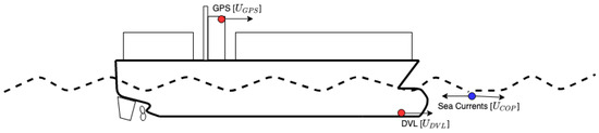
Figure 1. Locations where the three speed signals of interest derive from. Red is used to indicate ship sensors and blue for predictions.

Assuming an additive measurement error we obtain the following observed variables:

$$\begin{array}{cc}\hfill U_{GPS}& =U_g^b+{ϵ}_g\hfill \end{array}$$

(2)

$$\begin{array}{cc}\hfill U_{DVL}& =U_w^b+{ϵ}_w\hfill \end{array}$$

(3)

$$\begin{array}{cc}\hfill U_{COP}& =U_c^b+({ϵ}_c+{ϵ}_{\psi })\hfill \end{array}$$

(4)

It is assumed that each measured signal is mutually independent and affected by zero mean white Gaussian noise with variance ${\sigma }_g^2$ i.e., ${ϵ}_g\sim \mathcal{N}(0,{\sigma }_g^2)$, ${\sigma }_w^2$ i.e., ${ϵ}_w\sim \mathcal{N}(0,{\sigma }_w^2)$, ${\sigma }_c^2$ i.e., ${ϵ}_c\sim \mathcal{N}(0,{\sigma }_c^2)$ and ${\sigma }_{\psi }^2$ i.e., ${ϵ}_{\psi }\sim \mathcal{N}(0,{\sigma }_{\psi }^2)$. $\psi$ refers to ship’s compass true heading and is furthered analyzed in Section 2.1.

2. Fundamentals and Methodology

2.1. Theoretical Background of Position and Speed Signals

At this point, it is imperative to analyze each error term of Equations (2)–(4). Starting from Equation (2) the GPS gets the data from a GNSS (Global Navigation Satellite System) receiver providing synchronous measurements of ship position $(N_{lat},E_{lon})$ and SOG $\left(U_{GPS}\right)$. Most of the manufacturers of the GPS installed on company-owned ships, claim that the position accuracy accounts for ${\sigma }_p<2.5$ m. Only a few of them indicate the SOG accuracy. In one datasheet the SOG accuracy was registered for ${\sigma }_g<0.13$ kn.

Progressing to Equation (3) regarding DVL accuracy, numerous DVL manufacturers provide diversified information. Once calibrated the DVL measurements may approach an accuracy of $0.1$% [19], but a series of factors influence the result. Many DVL manufacturers claim that the accuracy is related to speed intensity followed by the below boundaries.

$$\left\{\begin{array}{c}\begin{array}{c}\hfill U_{DVL}<10\mathrm{kn}{\sigma }_w=0.1\mathrm{kn}\\ \hfill 10\mathrm{kn}\le U_{DVL}<25\mathrm{kn}{\sigma }_w=0.16\mathrm{kn}\\ \hfill 25\mathrm{kn}\le U_{DVL}<50\mathrm{kn}{\sigma }_w=0.32\mathrm{kn}\end{array}\hfill \end{array}\right.$$

Below are the factors influencing the DVL measurements, according to [6]:

• Water Clarity. The STW measurements depend on acoustic reflection from solid particles in the water such as microorganisms or suspended dirt. In extremely clear water the quantity of scatters may be insufficient for adequate signal return.
• Aeration. Aerated water under the transducer may reflect sound energy which could erroneously be interpreted as sea bottom returns. Sailing in heavy weather may be the source of this effect and so could non-laminar flow around the transducer. By placing the transducer near the bow the effect of non-laminar flow is reduced considerably.
• Ship’s trim and list. Changes in the trim (affects fore/aft speed) and list (affects transverse speed) of the ship will affect the measured speed. (e.g., $5^{\circ }$ trim change foresees 0.4% speed change [6]).
• Current profile. STW is measured relative to a water layer beneath the ship (>3 m). Sailing in strong tides and currents, the direction and magnitude of the surface current can be different from the measured layer, which may lead to errors in the measured speed.
• Eddy currents. Sailing in eddies in boundaries of ocean currents where the flow can be opposite or normal to the direction of the primary current may affect the speed measurement.
• Sea state. Following seas result in a variable change in the ship’s speed. This produces a fluctuation in the measured speed.
• Fouling of sensor. Fouling affects the sensor in the same way as the rest of the wetted surface of the ship.

Lastly, Equation (4) assumes that $U_{COP}$ is subject to two error terms, ${ϵ}_c$ and ${ϵ}_{\psi }$. The first is a combination of prediction error from the grid provided by the external weather provider along with the error from the bi-linear interpolation to match the ship’s location to that grid. According to CMEMS (Copernicus Monitoring Environment Marine Service) [20] ${\sigma }_c=0.37$ kn. The latter is the error deriving from the projection of the sea currents speed vector ${\mathbf{U}}_c^n={[U_x,U_y,0]}^{\mathrm{T}}\in {\mathbb{R}}^3$ to the ship’s true heading measurements ${\psi }_m$. ${\psi }_m$ is a measurement provided by the gyrocompass installed on the ship. Observation at sea indicates that ${0.25}^{\circ }$ is the error in many typical gyrocompass installations [21]. Consequently, invoking the gyrocompass error into the projection formula, it derives that ${\sigma }_{\psi }=0.001$ kn. To sum up, the measurements have been identified with error characteristics as stated in Table 1. The present study is trying to showcase how far or close to reality the error values of Table 1 are.

Table 1. Estimated accuracy ($1\sigma$) of motion and weather signals, according to manufacturers or weather providers’ documentation [19,20,21].

Signal	Accuracy [$\mathit{\sigma }$]
$N_{lat},E_{lon}$	$2.5\left[\mathrm{m}\right]$
$U_{GPS}$	$0.13\left[\mathrm{kn}\right]$
$U_{DVL}$	$0.16\left[\mathrm{kn}\right]$
$U_{COP}$	$0.37\left[\mathrm{kn}\right]$

2.2. Error Identification in STW Measurement

It is imperative to develop a detailed explanation of how to check potential error in the STW measurement. Based on Equations (1)–(4) we obtain:

$$\begin{array}{cc}\hfill U_{dev}& =U_{GPS}-U_{DVL}\hfill \\ \hfill & =U_{COP}\hfill \end{array}$$

(5)

Equation (5) indicates that there is a speed deviation which we can easily calculate by subtracting the measured STW ($U_{DVL}$) from SOG ($U_{GPS}$) and it must be equal to the projected speed of the currents ($U_{COP}$). According to [22], the range of magnitude of global currents, span from $0.01$ kn to $7.78$ kn. However, currents generally diminish in intensity with increasing depth, so the higher end of the magnitude range refers to shallow water currents close to shore. According to [23] a characteristic sea surface speed is $0.1$ kn to $0.97$ kn. More specifically, in 98% of the bins, the mean surface current did not exceed $0.97$ kn. After illustrating the GPS coordinates registered from 190 container ships during 3 years of operation in Figure 2, it is evident that liner shipping is following specific seaways unlike bulk and crude oil carriers. In Figure 3 there is an illustration from [22] depicting the global surface currents magnitude during northern hemisphere winter. When comparing the last two figures, it is indisputable that most of the ships’ seaways are along one of the streams. Considering the above, in this research study we have assumed that a container ship sailing in steady state is unlikely to confront (from any direction) a surface current speed magnitude ${\mathbf{U}}_c^n=\sqrt{U_x^2+U_y^2}$ greater than $2.0$ kn, which is the value of the defined threshold referred to in Section 1.3.

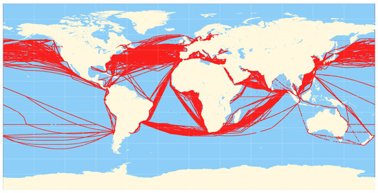
Figure 2. Visualization of $N_{lat}$ and $E_{lon}$ coordinate pairs from all ships included in the main dataset for 3 years of operation.

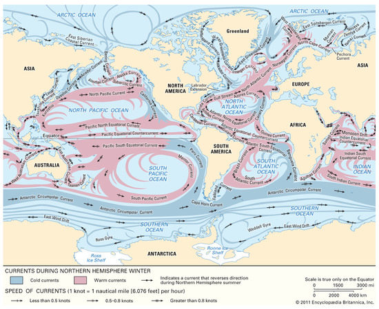
Figure 3. Global surface currents magnitude during northern hemisphere winter by [22].

Focusing down to a single ship level, the same $2.0$ kn threshold can be used to identify if the STW and SOG measurements are experiencing significant errors. The procedure is the following:

• Acquire STW measurements, SOG measurements and high resolution (both spatial and temporal) sea currents reanalysis outputs obtained by a weather provider.
• Create a scatterplot of SOG vs. STW and inspect the correlation of the two vectors. They are expected to be highly correlated.
• Create the speed deviation feature $U_{dev}$ which is a product of subtracting STW from SOG like Equation (5), plot a histogram and a boxplot to check the distribution of $U_{dev}$ and calculate the percentage of $|U_{dev}|>2$ kn.
• Plot the histogram and boxplot of $U_{COP}$ to check its distribution and identify the statistical characteristics of the sea currents magnitude of the regions where the ship has sailed. Plot the ship seaways on a map to verify if the $U_{COP}$ values reflect the characteristics of the sea region.
• Compare $U_{dev}$ and $U_{COP}$ distributions. When the $U_{dev}$ boxplot of one ship’s median is close to 0, the inter-quantile range (IQR) is narrow enough to span from $-1$ to 1 knot, and the whiskers span between $-2$ and 2 knots, and finally the $U_{COP}$ distribution conveys the same story then it is indicative that the DVL measurements can be trusted. Anything outside these boundaries is questionable and requires further investigation by location.

At this point, it should be noted that the particular threshold value of 2 kn is a decision made by the authors. The investigations made in relation to the strength of average sea current, indicate that the 2 kn threshold is a reasonable choice/decision. It is expected that the outcome of the analysis to some degree depends on the precise value of the threshold and, as such, there is incentive for making a sensitivity study to comprehensively investigate the influence of the threshold value on the outcome and findings. However, this exercise is beyond the scope of the present paper and is left as a work for the future.

3. Data

3.1. Sources

As already introduced, data has been collected from many different sources; both internally (within the company) and externally (open-source as well as paid services). Below are the descriptions of each available data source that has been meticulously merged to end up in the final dataset.

3.1.1. CAMS Data

This study is conducted on sensor data from Maersk’s fleet deriving from a system called CAMS (Control Alarm Monitoring System). Thus, CAMS is the source of the main dataset and it includes sensor readings from each ship. CAMS contains 10-min sampled data from all distributed sensors along the ships, and is sent to shore continuously as often as there is satellite connection available on-board each ship. There are around 300 variables available in CAMS but only a subset of these are a priori assumed to affect the STW sensor readings and thus included in this study. In CAMS, each ship is identified by its unique IMO number, and Table 2 illustrates the chosen features for each of the downloaded IMO numbers.

Table 2. Sampling frequency, acquisition range and units of CAMS data.

Condition	Type	Frequency	Range	Unit
Loading	Draught Aft	$0.001$ Hz	0–30	[m]
	Draught Fore	$0.001$ Hz	0–30	[m]
Operational	GPS Timestamp	$0.001$ Hz	14/12/2016–22/02/2020	[UTC datetime]
	Latitude	$0.001$ Hz	$-90$–90	[${}^{\circ }$]
	Longitude	$0.001$ Hz	$-180$–180	[${}^{\circ }$]
	Shaft speed	$0.001$ Hz	$-300$–300	[rpm]
	ME Power	$0.001$ Hz	0–100,000	[kW]
	Longitudinal STW	$0.001$ Hz	$-10$–50	[kn]
	GPS SOG	$0.001$ Hz	$-10$–50	[kn]
	True heading	$0.001$ Hz	0–360	[${}^{\circ }$]
	Course over ground	$0.001$ Hz	0–360	[${}^{\circ }$]
	Roll	$0.001$ Hz	$-90$–90	[${}^{\circ }$]
	Pitch	$0.001$ Hz	$-90$–90	[${}^{\circ }$]
	Water Depth (Under Keel)	$0.001$ Hz	0–11,000	[m]
Weather	True Wind Speed	$0.001$ Hz	0–50	[m/s]
	True wind direction	$0.001$ Hz	0–360	[${}^{\circ }$]
	Relative wind speed	$0.001$ Hz	0–50	[m/s]
	Relative wind direction	$0.001$ Hz	0–360	[${}^{\circ }$]
	Sea temperature	$0.001$ Hz	$-50$–100	[°C]

3.1.2. AIS Data

The AIS is an automatic tracking system that uses transceivers on ships and is used by vessel traffic services (VTS). AIS information supplements marine radar, which continues to be the primary method of collision avoidance for water transport. It is confirmed that AIS is using a different set of sensors than the CAMS dataset. This means that all available measurements are comparable with the adequate CAMS measurements. The company does not collect this data, but an external provider does, and it is where the data was sourced from. The AIS dataset is used for comparison and correction purposes mainly due to faulty GPS locations registered on the CAMS dataset. Table 3 show the selected features from the AIS dataset.

Table 3. Sampling frequency, acquisition range and units of AIS data.

Condition	Type	Frequency	Range	Unit
Loading	Draught Avg	uneven	0–30	[m]
Operational	AIS Timestamp	uneven	01/10/2017–10/03/2020	[UTC datetime]
	AIS SOG	uneven	$-10$–50	[kn]
	Latitude	uneven	$-90$–90	[${}^{\circ }$]
	Longitude	uneven	$-180$–180	[${}^{\circ }$]
	True heading	uneven	0–360	[${}^{\circ }$]
	Course over ground	uneven	0–360	[${}^{\circ }$]

3.1.3. IHO Seas Data

There is a report from IHO (International Hydrographic Organization) called “Limits of oceans and seas in digitized, machine readable form" [24] which includes the boundaries of 148 oceans and seas. The given positions were typed into a spreadsheet and were completed to a right ordered polygon by hand using Google Earth. This dataset is the digitized version of the printed “Limits of Oceans and Seas" [25]. The dataset is structured by the columns as described in Table 4 and will help classify the STW accuracy issue into regional categories. In Figure 4 one can see the borders of each sea as reference.

Table 4. Sampling frequency, range and units of IHO seas data.

Condition	Type	Frequency	Range	Unit
Sea info	Sea name	1 name/sea	148 seas worldwide.	[-]
	Geometry	1 polygon/sea	148 unique geopolygons	[-]
	Area	1/polygon	$0.16$–$7512.32$	[${\mathrm{km}}^2\ast {10}^2$]

Figure 4. The IHO seas regions of the world.

3.1.4. General-Info Data

Following the same classification principle, particular information for each ship of the dataset is provided through an internal company source. For instance, the vessel class and the DVL manufacturers info are some of the features out of a range of valuable categorical variables that has helped classify the data and identify if they relate to the STW accuracy. The classification dataset named from now on the ’general-info’, is shown in Table 5.

Table 5. Sampling frequency, range and units of general-info data.

Type	Frequency	Range	Unit
Vessel name	1/ship	224 ship names	[-]
Vessel IMO No	1/ship	224 unique numbers	[-]
Vessel class	1/ship	32 ships classes	[-]
Vessel flag	1/ship	6 flags	[-]
DVL manufacturer	1/ship	6 manufacturers	[-]
DVL model	1/ship	28 unique models	[-]

3.1.5. Hull and DVL Cleaning Events

According to [26] sensor fouling has proved to be one the more influencing factors on the quality of the DVL measurements. Based on this assumption the hull and DVL cleaning events of each ship over time has been included in the study. Especially the timestamps where the cleaning and re-calibration of the DVL take place are expected to be significant and might reveal high correlation with $U_{dev}$. Table 6 describes the dataset for each ship. The length of the table depends on the amount of cleaning events registered for each ship.

Table 6. Sampling frequency, range and units of cleaning events data.

Type	Frequency	Range	Unit
Event name	total number of events/ship	8 unique events	[-]
Event location	total number of events/ship	21 unique locations	[-]
Event timestamp	total number of events/ship	20/12/1979–26/02/2020	[UTC datetime]

3.1.6. MET Ocean Data

MET ocean data is sourced from external providers. In this study, MET ocean data includes information about sea current and waves, and in either case data is collected with credit to the E.U. Copernicus Marine Service Information. Specifically, sea current was obtained from CMEMS [27] while wave data relies on ERA5 [28]. ERA5 is a reanalysis database that provides hourly updates of wave spectra in grid points spaced by ${0.5}^{\circ }$ latitude and longitude degrees. Table 7 presents the features downloaded and later bi-linearly interpolated using the method described in [29].

Table 7. Temporal and spatial resolution, acquisition range and units of weather data. * Sig.wave height refers to the significant height of combined wind waves and swell. ** SMOC refers to Surface and Merged Ocean Currents.

	Type	Temp. Res.	Spat. Res.	Range	Unit
ERA5	ERA5 Timestamp	-	-	01/01/1979–present	[UTC datetime]
	Sig.wave height *	hourly mean	${0.5}^{\circ }\times {0.5}^{\circ }$	0–20	[m]
	Mean wave period	hourly mean	${0.5}^{\circ }\times {0.5}^{\circ }$	0–100	[s]
	Mean wave direction	hourly mean	${0.5}^{\circ }\times {0.5}^{\circ }$	0–360	[${}^{\circ }$]
CMEMS	CMEMS Timestamp	-	-	01/01/1992–present	[UTC datetime]
	SMOC utotal **	hourly mean	${0.083}^{\circ }\times {0.083}^{\circ }$	$-20$–20	[kn]
	SMOC vtotal **	hourly mean	${0.083}^{\circ }\times {0.083}^{\circ }$	$-20$–20	[kn]

The sea current velocity vector measurements, combined with the true heading of the ship as given by compass ${\psi }_m$, one can find the projected speed of the currents on the ship’s body-fixed reference frame $U_{COP}$.

3.2. Data Processing

This section describes the preprocessing of the data. Although this task is an asynchronous process, below is an ordered description of the steps that ended up to the main (final) dataset.

3.2.1. Filtering and Merging

Focus is exclusively on the actual sailing operations. Thus, many of the other parts of shipping operations are filtered out; this includes quay stays, anchoring, maneuvering, maintenance (dock stays), etc. In practice, this was simply done by including data only if the forward speed is above 5 knots, although important information such as cleaning events and dock stays were kept track of. In total, the dataset was reduced to 40% of the original dataset.

Since CAMS is the main dataset, the rest of the data sources are merged to this. Figure 5 illustrates the merging of the rest of the data sources to the CAMS dataset. In cases where there were no exact timestamp match, a tolerance level of a few seconds is given, depending on the importance of the related merged features. For cleaning events, the merging led to a new feature counting the number of days since the last occurrence of each of those events. In cases where the frequency of the merged dataset was lower than that of the main dataset, the merging resulted in missing data which needed to be imputed. Depending on each feature’s physical properties, the replacement of the missing data has been handled adequately as described in the next subsection.

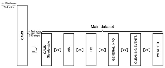
Figure 5. An illustration of the merging procedure of the data sources.

3.2.2. Outlier and Missing Data Replacement

Most of the missing values of the main dataset derived either from CAMS or from the merging process. In Figure 6 one can see the missing data matrix for the most significant features of the main dataset. It starts on 01-01-2017 and ends on 22-02-2020 and it sums up to 190 ships and ≈7 million rows.

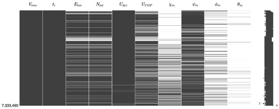
Figure 6. Missing data matrix for the principal features of the main dataset.

It is illustrated in Figure 6 that from the 7,333,490 rows of the dataset, the GPS coordinates $N_{lat}$ and $E_{lon}$ have several missing values ($15\%$) after validating and correcting the measurements with AIS data. For other parameters (return to the nomenclature for notation), the following can be noted: ${\psi }_m$ has $14\%$ missing values due to malfunction of the compass on some ships, ${\theta }_m$ has $97\%$, ${\varphi }_m$ has $81\%$, ${\chi }_m$ has $71\%$, $U_{dev}$ has $0.5\%$ missing values deriving from random iterations of $U_{DVL}$ missing values, and finally $U_{COP}$ has ($25\%$) missing values deriving from $N_{lat}$, $E_{lon}$ and ${\psi }_m$. Here, it should be noted that the features, with missing values-percentages higher than >70%, have been dropped entirely from the main dataset.

Each feature of the main dataset has been meticulously checked for outliers. This includes obvious outliers based on physical constraints, drop-outs, spikes and finally repeated values indicating frozen signals. The methodology followed on identifying outliers was based on the work by Dalheim and Steen [30].

After identifying missing values and outliers followed a careful replacement process. In fact, the replacement has been one of the most tedious tasks of this study, because the replaced values had to be validated for all ships. Even a small mistake might lead to wrong conclusions on the analysis and the modeling section. For instance, when latitude and longitude outliers were identified in CAMS, they were replaced with their AIS substitute, since it has been internally investigated that the AIS system uses a dedicated GNSS antenna separate from the one that the ship uses for the GPS coordinates. However, there were cases that even the substituted values did not comply with the validation constraints. In these cases, it was decided to linear interpolate instead of creating an additional filter where the location would be estimated based on a physical model.

3.2.3. Main (Final) Dataset

Table 8 describes all the main features of interest that constitute the main dataset. This dataset has been used for the analysis and modeling part. Some features had to be dropped from the main dataset after the merging, either because of the high number of missing values, or because they were assumed to be less significant for the purpose of this study. Please note that the sampling frequency of ships on the main dataset is uneven, since the maneuvering state has been completely dropped.

Table 8. Type, symbol, short description, value range and units for final dataset. For longer description, refer to the table at Nomenclature.

Type	Symbol	Short Description	Range	Unit
Time	$t_i$	Timestamp	14/12/2016–22/02/2020	[UTC datetime]
Motion	$N_{lat}$	Latitude	$-50$–61	[${}^{\circ }$]
	$E_{lon}$	Longitude	$-180$–180	[${}^{\circ }$]
	${\psi }_m$	True heading	0–360	[${}^{\circ }$]
	$U_{DVL}$	STW	0–29	[kn]
	$U_{GPS}$	SOG	5–28	[kn]
	$U_{dev}$	Speed deviation	$-10$–10	[kn]
	$U_{COP}$	See currents speed	$-6$–6	[kn]
	$D_{avg}$	Draught Avg	1–29	[m]
Engine	$E_{rpm}$	ME Shaft rotations	30–101	[rpm]
	$E_{pow}$	ME Power	0–65,574	[kW]
Environmental	$S_{temp}$	Sea temperature	1–49	[°C]
	$S_{depth}$	Water Depth (Under Keel)	0–8086	[m]
	$H_{sw}$	Significant wave height	0–13	[m]
	$d_{sw}$	Mean wave direction	0–360	[${}^{\circ }$]
	$U_{rw}$	Relative wind speed	0–50	[m/s]
	$d_{rw}$	Relative wind direction	0–360	[${}^{\circ }$]
Classifiers	$S_{name}$	Sea name based on region	Categorical	[-]
	$M_{sl}$	DVL manufacturers	Categorical	[-]
	$V_{class}$	Vessel class	Categorical	[-]
	$V_{imo}$	Unique ImoNo per vessel	Categorical	[-]
Cleaning Events	$C_{bov}$	Days since birth of vessel	46–7935	[days]
	$C_{ddp}$	Days since last dry docking (painting)	0–5000	[days]
	$C_{ddfb}$	Days since last dry docking (full blast)	0–5000	[days]
	$C_{pp}$	Days since last propeller polishing	0–5000	[days]
	$C_{hc}$	Days since last hull cleaning (locally)	0–5000	[days]
	$C_{la}$	Days since last DVL adjustment	0–5000	[days]

4. Analysis and Modeling

In this section, the main dataset has been analyzed, attempting to answer the research questions. The section starts with the $U_{dev}$ and $U_{COP}$ decompositions over the whole fleet (Section 4.1 and Section 4.2) and proceeds with a regression analysis of the main features of interest versus $U_{dev}$.

4.1. $U_{dev}$ Decomposition

In Section 2.2 we assumed that a container ship sailing in open waters is unlikely to confront a surface current speed ${\mathbf{U}}_c^n$ greater than 2 kn. Hence the threshold of 2 kn is used to identify potential errors of the STW and SOG measurements. It is otherwise expected that $U_{DVL}$ and $U_{GPS}$ are linearly correlated. The scatterplot in Figure 7 depicts the correlation of the two features deriving from the whole fleet. The red-colored dots indicate those indices that are outside the speed deviation boundary of 2 knots ($|U_{dev}|>2$ kn). At first glance there seems to be many faulty indices (red dots) in the CAMS dataset. However, when looking at the bivariate kernel density estimate (KDE) plotted on top of the scatterlot, it is evident that the issue is not that severe, since most of the points are concentrated within five contour levels below $2.0$ kn within the gray area.

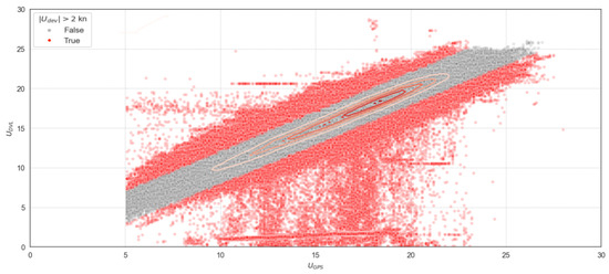
Figure 7. KDE plot on top of correlation scatterplot of $U_{GPS}$ versus $U_{DVL}$ from 190 container ships.

Checking on the percentage of points distributed among the 2 kn boundary, on Table 9 one can see that only $2.47$% out of ≈7 million points are considered to be either DVL or GPS failure. Even small fractions of DVL failure can contribute to huge costs, especially for companies operating hundreds of ships.

Table 9. Speed deviation $U_{dev}$ above and below 2 kn boundary.

	$|{\mathit{U}}_{\mathit{d}\mathit{e}\mathit{v}}|<2$ kn	$|{\mathit{U}}_{\mathit{d}\mathit{e}\mathit{v}}|>2$ kn	total
count	7,152,295	181,195	7,333,490
percentage%	$97.53$%	$2.47$%	100%

However, given that 2.47% out of ≈7 million measurements is experiencing faulty DVL and GPS measurements, one can decompose Table 9 by vessel class and by DVL manufacturer and inspect how much above or below this general percentage boundary each category is sitting. Table 10 and Table 11 reports the outcome of this analysis for DVL manufacturer and vessel class.

Table 10. Speed deviation $U_{dev}$ above 2 kn boundary decomposed by DVL manufacturer installed on the 190 ships of this study. Gray background occurs when $|U_{dev}|>2$ kn percentage column is greater than $2.47\%$.

Manufacturers	$|{\mathit{U}}_{\mathit{d}\mathit{e}\mathit{v}}|>2$ kn		Total
	count	perc %
NaN	52,000	$2.67$%	1,947,949
M.1	33,878	$1.81$%	1,871,659
M.2	32,254	$2.43$%	1,325,151
M.3	13,450	$1.85$%	727,145
M.4	11,068	$1.79$%	618,358
M.5	32,946	$5.36$%	614,225
M.6	5599	$2.44$%	229,003

Table 11. Speed deviation $U_{dev}$ above 2 knots boundary decomposed by vessel class. Gray background shows up when $|U_{dev}|>2$ kn percentage column is greater than $2.47\%$ and it gets darker while it increases.

Vessel Class	$|{\mathit{U}}_{\mathit{d}\mathit{e}\mathit{v}}|>2$ kn		Total
	count	perc %
C.7	21,047	$1.56$%	1,346,739
C.26	24,727	$1.98$%	1,251,124
C.15	14,075	$1.72$%	816,046
C.9	7955	$1.45$%	548,497
C.16	19,651	$3.51$%	559,411
C.12	13,174	$3.26$%	404,647
C.10	12,024	$3.55$%	338,794
C.11	5293	$1.85$%	285,827
C.14	13,087	$4.97$%	263,230
C.24	2162	$1.17$%	184,113
C.27	943	$0.52$%	180,521
C.3	1784	$1.10$%	161,798
C.2	6500	$4.72$%	137,575
C.4	6834	$5.16$%	132,552
C.17	2300	$1.96$%	117,575
C.13	10,557	$9.20$%	114,694
C.21	1487	$1.79$%	83,068
C.5	991	$1.43$%	69,454
C.23	4641	$6.61$%	70,161
C.18	1468	$2.33$%	62,934
C.6	1145	$1.93$%	59,429
C.22	818	$1.74$%	46,884
C.1	499	$1.22$%	40,939
C.20	559	$2.02$%	27,618
C.25	55	$0.47$%	11,745
C.19	2705	$20.19$%	13,401
C.8	4714	$100.00$%	4714

For anonymity, the brand names of the DVL manufacturers have been changed into index numbers. The only DVL manufacturer that is far above the $2.47\%$ boundary layer is M.5. Later, it has been confirmed that this is not a proof of a manufacturer of low accuracy, but this indication is caused by a few ships with miscalibrated or malfunctioning sensors at some period of time.

As seen in Table 11, there are a few vessel classes in which the percentage is greater than $2.47\%$ and these classes have been investigated thoroughly. Boxplots are used to illustrate the ship level, as illustrated in Figure 8.

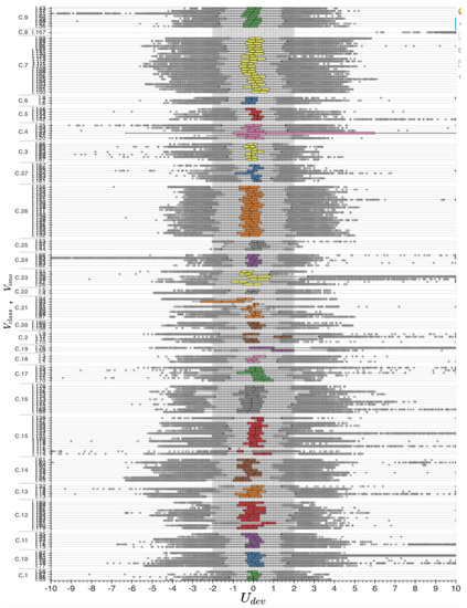
Figure 8. Boxplot of $U_{dev}$ by vessel class $V_{class}$ and IMO number $V_{imo}$.

It is evident that most of the ships’ IQRs span among $\pm 1$ kn. Some IQRs are narrower than others, which indicate that there is a stronger correlation between SOG and STW. Strong correlation implies either minimal signals error or that the ships sail in areas with very small or no ocean current. The latter is not likely, since ships from almost all vessel classes sail in at least one sea region where the sea currents happen to be stronger than average. Focusing on the vessel classes categorization, it seems that ships under the same class record similar performance. For instance, the boxplots from class C.16 (gray boxplots) look wider than those from class C.7 (yellow boxplots) meaning that the IQRs of C.7 imply stronger correlation between SOG and STW than those of C.16. Some boxplots from C.7 are shifted to the left, which means that the mean value is negative which implies that the ship is mostly confronted with head currents, where when it is shifted to the right, the mean value is positive, and it implies that the ship is mostly enjoying following currents. The whiskers of C.7 do not exceed $\pm 2$ kn where those of C.16 do that in some cases. Additionally, the outliers (which constitute only the $0.7\%$ of the data) of C.7 are more condensed than those of C.16 where one can see a few scattered cases to the right. Adding class C.26 into the comparison (orange boxplots) the IQRs there indicate that the correlation is similar to that of C.16 but the whiskers imply that the variance of the distribution is similar to that of C.7. In a few words, one can say that C.7’s measurements seem more trustworthy than those of C.26 which in turn seem more trustworthy than those of C.16 and so on.

Diving a bit deeper and splitting the boxplots using an additional dimension as on the tables earlier, say the DVL manufacturers, one can see the resemblance or differences. Figure 9 depicts the additional split. For instance, when focusing on class C.15, one can clearly see that each ship wears one of the two different DVL manufacturers (NAN refers to missing values). There is a slight difference in the IQR between the two sets of boxplots. Those of M.1 are a bit narrower than the others. Also, all whiskers of M.1 are within the $\pm 2$ kn boundary where some of the others span beyond it.

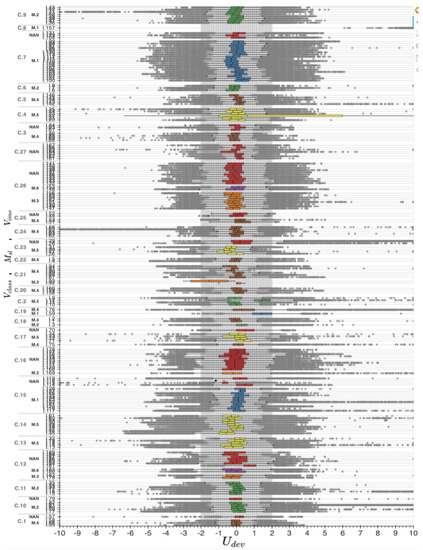
Figure 9. Boxplot of $U_{dev}$ by vessel class $V_{class}$, DVL manufacturer $M_{sl}$ and imoNo $V_{imo}$.

To combine the table information of the boundary percentage of $2.47\%$ with the boxplots, it can be appreciated from Figure 10 in which ships the boundary percentage is exceeded (after the dashed-black-line). Getting back to the C.7–C.16 class example from above, when one checks the percentage of $U_{dev}$ which goes beyond 2 kn in Figure 10, the advantage of C.7 over C.16 class is evident. C.7 ships never exceed the general percentage boundary of $2.47\%$. On the other hand, there are several C.16 class ships that exceed the percentage boundary layer. This is because some whiskers of C.16 class boxplots of Figure 8 span beyond the ±2 kn boundary limit. Same goes with class C.26 where only one ship exceeds the boundary percentage.

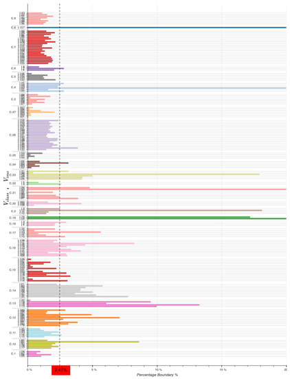
Figure 10. Barplot of $U_{dev}$ boundary percentage by vessel class $V_{class}$ and IMO number $V_{imo}$.

Another categorical feature of the main dataset that is interesting to investigate is the sea region. Due to space limitations, Table 12 shows only the seas where the percentage of $|U_{dev}|>2$ kn column was above the $2.47\%$ boundary. It is evident from the percentage column that most of the seas with the highest scores refer to either narrow passages or shallow water regions.

Table 12. Speed deviation $U_{dev}$ above 2 kn boundary decomposed by sea name where the ships have been sailing. Only those seas where the percentage column is greater than $2.47\%$ have been included. Gray background gets darker when the percentage column of $|U_{dev}|>2$ kn increases.

Sea Region	$|{\mathit{U}}_{\mathit{d}\mathit{e}\mathit{v}}|>2$ kn		Total
	count	perc %
North Atlantic Ocean	30,656	$3.35$%	913,938
Indian Ocean	29,353	$3.50$%	839,133
Arabian Sea	9223	$2.56$%	360,849
North Sea	6103	$4.21$%	145,058
English Channel	14,413	$17.01$%	84,719
Japan Sea	1764	$3.17$%	55,680
Alboran Sea	2783	$5.61$%	49,586
Gulf of Mexico	2040	$6.01$%	33,947
Andaman or Burma Sea	1740	$6.25$%	27,835
Philippine Sea	2710	$13.86$%	19,548
Gulf of St. Lawrence	843	$5.21$%	16,179
Ionian Sea	281	$3.18$%	8840
Strait of Gibraltar	1925	$26.20$%	7346
Singapore Strait	586	$8.81$%	6648
Coral Sea	766	$12.55$%	6104
Rio de La Plata	133	$3.66$%	3633
Tasman Sea	468	$14.41$%	3247
Java Sea	236	$14.33$%	1647
Arafura Sea	150	$12.08$%	1242
Gulf of Thailand	45	$3.66$%	1228
Great Australian Bight	104	$25.18$%	413
Bass Strait	35	$14.17$%	247

By depicting the seas on the map, the above statement gets even clearer. Figure 11 highlights the sea regions with high percentage boundary in gray scale, same as in Table 12. The greatest amounts are occupied by North Atlantic Ocean, Indian Ocean and Arabian sea but as seen by the color scale, these are the least alarming regions. The percentage is increasing when ships have sailed around Oceania, Philippines, Singapore and in short passages where sea currents are known to be stronger than the rest of the world, such as the English Channel and the Strait of Gibraltar.

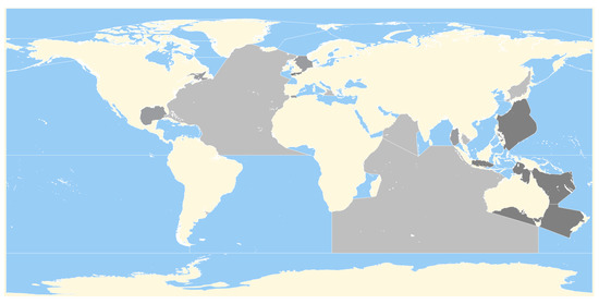
Figure 11. The IHO seas regions of the world. The regions are gray when the percentage column of $|U_{dev}|>2$ kn is greater than $2.47\%$ and it gets darker when it increases.

4.2. $U_{COP}$ Decomposition

According to (5), $U_{dev}$ and $U_{COP}$ should be equal. In case there is any deviation between them, it should be due to a mix of measurement and prediction error from GPS, DVL, compass and sea currents. Checking on the percentage of points distributed among the 2 kn boundary for $U_{COP}$, on Table 13 it is realized that only $0.63\%$ out of $\approx 7$ million points from ships sailing across the global seas has experienced a stronger current than 2 kn on its bow.

Table 13. Sea currents predicted speed $U_{COP}$ above and below 2 kn boundary.

	$|{\mathit{U}}_{\mathit{C}\mathit{O}\mathit{P}}|<2$ kn	$|{\mathit{U}}_{\mathit{C}\mathit{O}\mathit{P}}|>2$ kn	Total
count	7,287,465	46,025	7,333,490
percentage%	$99.37$%	$0.63$%	100%

The percentage compared to the one from $U_{dev}$ is significantly smaller. This means that the predicted sea currents deriving from the external provider, deviate from the ones calculated by the measured GPS and DVL resulting in $U_{dev}$. The above statement implies that it is either (i) the external provider that is underestimating the truth about the surface sea currents magnitude, (ii) the signal errors provided by the manufacturers of GPS, DVL and gyrocompass sensors are a lot higher than what they disclose, or (iii) there is a deeper layer of sea currents predictions $U_{CO{P}_d}$ which resembles more with $U_{dev}$ than with $U_{COP}$. In other words, case (iii) assumes that the DVL sensor measures the STW by viewing the speed of the currents on a deeper layer rather than the surface. If at some regions the deeper layer differs in magnitude and direction from the surface layer, then case (iii) is the most reasonable explanation. The inference of this is that it could be relevant to make an investigation where depth is considered to be a third dimension on the global sea currents. Although this exercise is left for the future, some initial investigations have been made [31].

Placing the distributions of $U_{dev}$ and $U_{COP}$ side-by-side in Figure 12, one can see the difference between them.

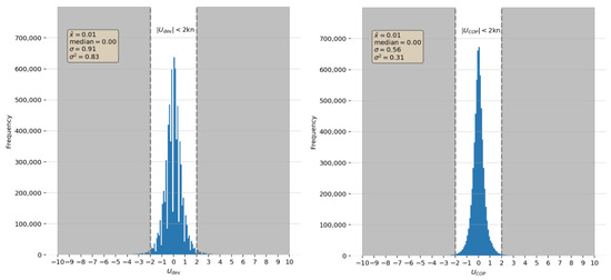
Figure 12. Distribution histograms of $U_{dev}$ and $U_{COP}$ for 190 container ships.

Both are symmetrical distributions with similar mean and median, and different variance. Enhanced with the boxplots of Figure 13 it is easy to distinguish a few points. First, the $U_{COP}$ distribution perfectly coincide with the claims from [23,32] which is a confirmation that the sea currents affecting the ships of that study match with the generic global statistics of surface currents. Secondly, there are a lot of outliers on the $U_{dev}$ distribution that are not present in $U_{COP}$. From Equation (5), and based on Table 1 and the above distributions, it is assumed that the error of $U_{dev}$ is greater than that of $U_{COP}$ which means that ${ϵ}_w$ and ${ϵ}_g$ is greater than ${ϵ}_{\psi }$ and ${ϵ}_c$ despite what the manufacturers and weather providers claim. Given that ${ϵ}_g$ is low because of the high accuracy of the GPS receiver [33], the highest difference is assumed to be derived from the DVL error ${ϵ}_w$.

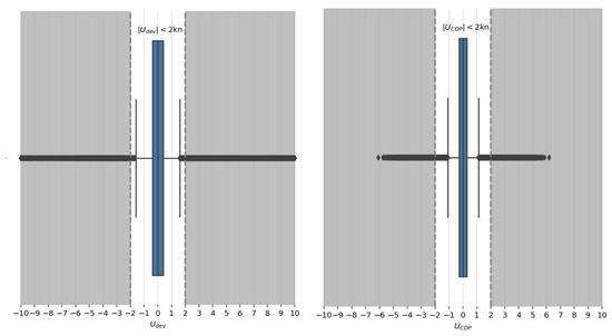
Figure 13. Distribution boxplots of $U_{dev}$ and $U_{COP}$ for 190 container ships.

By using the same approach as with $U_{dev}$, $U_{COP}$ can be similarly decomposed by category. The distribution by sea name is the most relevant, because sea currents ought to be related to sea regions, as presumed by Figure 3. In Table 14 one can see what the percentage is of $U_{COP}$ that is above or below the initially defined 2 kn boundary.

Table 14. Sea surface currents speed projection on ship’s true heading $U_{COP}$ above 2 kn boundary decomposed by sea name where the ships have been sailing. Only those seas where the percentage column is greater than $0.63\%$ have been included. Gray background gets darker when the percentage column of $|U_{COP}|>2$ kn increases.

Sea Region	$|{\mathit{U}}_{\mathit{C}\mathit{O}\mathit{P}}|>2$ kn		Total
	count	perc %
North Atlantic Ocean	6001	$0.66$%	913,938
Indian Ocean	16,832	$2.01$%	839,133
South China Sea	7769	$1.44$%	539,339
Malacca Strait	2306	$1.17$%	196,523
North Sea	2385	$1.64$%	145,058
English Channel	2374	$2.80$%	84,719
Japan Sea	818	$1.47$%	55,680
Gulf of Mexico	595	$1.75$%	33,947
Philippine Sea	1068	$5.46$%	19,548
Skagerrak	265	$1.49$%	17,745
Strait of Gibraltar	51	$0.69$%	7346
Singapore Strait	135	$2.03$%	6648
Mozambique Channel	11	$0.66$%	1668
Java Sea	11	$0.67$%	1647

It is a positive indication to see that most of the sea regions from Table 12 that were above the $2.47\%$ boundary percentage are again apparent in Table 14 with the new $U_{COP}$ boundary percentage of $0.63\%$. However, there are a few exceptions such as the Strait of Gibraltar, which in Table 12 conveys the impression that there are strong sea currents in the region ($26.20\%$ of $|U_{dev}|>2$ kn), but when compared with $U_{COP}$ of Table 14 the percentage ($0.69\%$ of $|U_{COP}|>2$ kn) does not validate the assumption. Figure 14 depicts the $U_{dev}$-$U_{COP}$ differences of all sea names in a boxplot format.

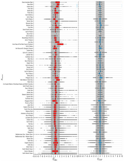
Figure 14. Barplots of $U_{dev}$ and $U_{COP}$ by sea name $S_{name}$.

Here, it is important to note that in regions with sea currents of high volatility such as the English Channel, it is peculiar to see a few outliers indicating a negative correlation between $U_{COP}$ and $U_{dev}$. This could be rationalized. The spatial resolution of the sea currents data is a ${0.083}^{\circ }\times {0.083}^{\circ }$ grid which means that when pointing at the Channel’s latitude (≈${50}^{\circ }$) the grid is ≈1.5 km wide. Given the fact that $U_{COP}$ is calculated by spatially interpolating into the two-dimensions grid ($1.5$ km $\times 1.5$ km) and later temporally interpolating (because of the frequency mismatch of the sensors with the external weather data) within whole hours, when the region is highly volatile in sea currents magnitude and direction (similar to the English Channel [34]), the calculation might generate some additional error and more outliers than usual. In Figure 15 there are two snapshot of the English Channel’s surface sea currents speed, one 2 hours after the other. Comparing the images, it is obvious that the magnitude and direction of the surface currents in the region are exposed to large variations. Pinpointing the sea regions by color of intensity in Figure 16 based on Table 14, one can see the differences and similarities of that with Figure 11.

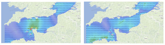
Figure 15. Snapshots of the English Channel sea currents ${\mathbf{U}}_c^n$ with 2-h difference from one another, by [35].

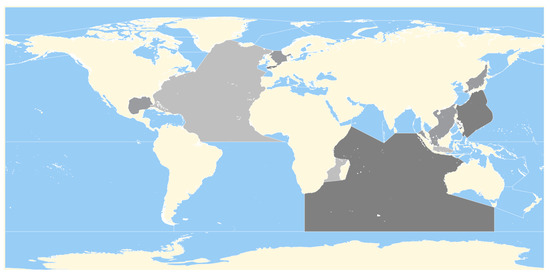
Figure 16. The IHO seas regions of the world. The regions are gray when the percentage column of $|U_{COP}|>2$ kn is greater than $0.63\%$ and it gets darker when it increases.

The boxplots of $U_{COP}$ by vessel class and IMO number have been plotted in Figure 17 to inspect and compare with $U_{dev}$ from Figure 8. By a first look at the $U_{COP}$ boxplots, it is clear that the IQRs are more condensed than those of $U_{dev}$. Additionally, almost all boxplots’ mean values are centered around 0 which is more likely than the shifted mean values from the $U_{dev}$ boxplots because almost all ships of the dataset have sailed for a long time window. There are a few exceptions though, such as the second ship from class C.21 with only a few iteration in the dataset. This ship’s boxplot is shifted to the left which implies strong head sea currents for as long as the data was recorded. Comparing the same ship’s boxplot from Figure 8, the ship was indeed under strong head currents. The question that rises again is which of the two is closer to what really happened.

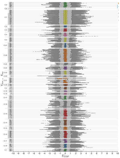
Figure 17. Boxplot of $U_{COP}$ by vessel class $V_{class}$ and IMO number $V_{imo}$.

Lastly, in Figure 17 one can distinguish the vessel classes that sail under calm versus strong sea currents. Class C.27 for instance, has mostly narrow boxplots compared to others. Indeed, C.27 ships sail mostly in Baltic sea where the sea currents are milder. There is one ship in C.27 in which the $U_{dev}$ boxplot’s mean does not match with the one from $U_{COP}$. In particular, the $U_{dev}$ mean is shifted to the left implying head sea currents for its entire journey. That ship’s data recordings span from 04/12/2018 to 22/02/2020 and in Figure 18 there is the $U_{dev}$ and the $U_{COP}$ for the whole journey. By comparing the two maps, it is more likely that the bottom is closer to the truth, because the Baltic sea currents look mild in the bottom map. On the contrary, in the upper map it seems like there is a constant head current during the whole journey which is highly unlikely. The apparent ship constitutes a proof that although $|U_{dev}|>2$ kn is below $2.47\%$, the error in STW is still high. This means that the 2 kn boundary initially set as a threshold for this study is quite sensitive in calm seas.

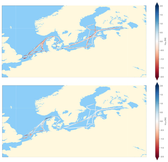
Figure 18. Full journey of a C.27 class ship from 04/12/2018 to 22/02/2020. Upper map shows a density plot of $U_{dev}$ where on the bottom map, the same for $U_{COP}$.

4.3. Regression Analysis

Two different correlation analyses have been used: (i) the Pearson correlation and (ii) the Spearman correlation. The first, evaluates the linear relationship, where the latter evaluates the monotonic relationship between two continuous features. A relationship is linear when a change in one feature is associated with a proportional change in the other feature. In a monotonic relationship, the features tend to change together, but not necessarily at a constant rate [36]. Figure 19 illustrates the Pearson and Spearman correlation matrices for the continuous features of the main dataset.

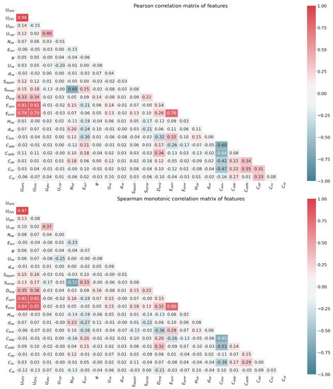
Figure 19. Pearson and Spearman correlation matrices of the continuous features of the main dataset.

As expected, $U_{GPS}$ and $U_{DVL}$ are highly correlated. Also, engine power $E_{pow}$ and engine shaft rotations $E_{rpm}$ are highly correlated with both $U_{GPS}$ and $U_{DVL}$. Next in correlation intensity is the sea temperature $S_{temp}$ with the latitude $N_{lat}$ which is also reasonable because sea temperature is warmer around the equator. Then, there is the feature that counts the number of days since the birth of the vessel $C_{bov}$ correlating with most of the cleaning events of the hull $C_{ddp}$, $C_{ddfb}$, $C_{pp}$ and $C_{hc}$. This is also straightforward since $C_{bov}$ is a constantly-increasing-over-time feature along with the rest of the cleaning features. Finally is the most unexpected low correlation pair, $U_{dev}$ with $U_{COP}$. This last one in a perfect world without measurement error, should be 1 since both $U_{dev}$ and $U_{COP}$ represent the same value.

Figure 20 depicts the linear relationships of all continuous features versus $U_{dev}$. On top of each scatterplot of the multi-graph, both the Spearman and Pearson correlation coefficients are indicated as titles. Focusing on the blue lines that represent the slope of each feature with $U_{dev}$, only on the third scatterplot with $U_{COP}$ is the line tilted, entailing linear relationship. In this scatterplot, it is also peculiar to see the great number of points concentrated around $U_{COP}=0$. This is an indication that even when the weather provider reports neutral sea surface currents, the speed sensors convey a different story.

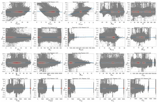
Figure 20. Linear correlation density scatterplot of $U_{dev}$ versus the rest of the continuous features of the main dataset.

The association between $U_{dev}$ and other explanatory variables such as $U_{GPS}$ is expected to be nonlinear. Due to complexity of the relationship between $U_{dev}$ and the rest of explanatory variables and due to the non-homogeneity of the variance of $U_{dev}$ it has been decided to run a GAMLSS (Generalized Additive Model for Location, Scale and Shape) for each of the continuous features of the main dataset. The GAMLSS is a modern distribution-based approach to (semiparametric) regression. A parametric distribution is assumed for the response (target) variable (in our case $U_{dev}$) but the parameters of this distribution can vary according to explanatory variables using linear, nonlinear or smooth functions [37]. Considering the GAMLSS model as:

$$\begin{array}{cc}\hfill \mathbf{Y}& \stackrel{ind}{\sim }\mathcal{D}(\mu ,\sigma ,\nu ,\tau )\hfill \\ \hfill {\mathit{\eta }}_1& =g_1\left(\mathit{\mu }\right)={\mathbf{X}}_1{\mathit{\beta }}_1+s_{11}\left({\mathbf{x}}_{11}\right)+\cdots +s_{1J_1}\left({\mathbf{x}}_{1J_1}\right)\hfill \\ \hfill {\mathit{\eta }}_2& =g_2\left(\mathit{\sigma }\right)={\mathbf{X}}_2{\mathit{\beta }}_2+s_{21}\left({\mathbf{x}}_{21}\right)+\cdots +s_{2J_2}\left({\mathbf{x}}_{2J_2}\right)\hfill \\ \hfill {\mathit{\eta }}_3& =g_3\left(\mathit{\nu }\right)={\mathbf{X}}_3{\mathit{\beta }}_3+s_{31}\left({\mathbf{x}}_{31}\right)+\cdots +s_{3J_3}\left({\mathbf{x}}_{3J_3}\right)\hfill \\ \hfill {\mathit{\eta }}_4& =g_4\left(\mathit{\tau }\right)={\mathbf{X}}_4{\mathit{\beta }}_4+s_{41}\left({\mathbf{x}}_{41}\right)+\cdots +s_{4J_4}\left({\mathbf{x}}_{4J_4}\right)\hfill \end{array}$$

(6)

where $\mathbf{Y}={(y_1,\cdots ,y_n)}^{\mathrm{T}}$ is the n length vector of the response variable, $\mathcal{D}(\mathit{\mu },\mathit{\sigma },\mathit{\nu },\mathit{\tau })$ is a four-parameter distribution, $\mathit{\mu },\mathit{\sigma },\mathit{\nu },\mathit{\tau }$ are the distribution parameters which are all vectors of length n, ${\mathit{\eta }}_k$ is the predictor vector for $k=1,2,3,4$, $g_k(.)$ are known monotonic link functions relating the distribution parameters to explanatory variables, ${\mathbf{X}}_k$ is a fixed known design matrix of order $n\times j$, ${\mathit{\beta }}_k$ is the coefficient vector, $s_{kj}$ is a non-parametric smoothing function applied to covariate ${\mathbf{x}}_{kj}$ for $j=1,\cdots ,J$ [38]. Parameter $\mu$ defines the location (mean), $\sigma$ the scale (standard deviation) and finally $\nu ,\tau$ define the shape (skewness and kurtosis) of the distribution.

In Figure 21 there is the multi-GAMLSS plot. In each sub-graph there is a continuous feature acting as the explanatory variable enhanced with the additive term of cubic smoothing splines with 5 effective degrees of freedom in all four parameters. Since only one explanatory variable is used in the fit, centile estimates for the fitted distribution are also plotted in each sub-graph, showing $0.4\%$, $2\%$, $10\%$, $25\%$, $50\%$, $75\%$, $90\%$, $98\%$ and $99.6\%$ centiles. The gray shade in between each consecutive boundary represents the segments of the distribution. For instance, $50\%$ of the distribution falls within the darkest gray area.

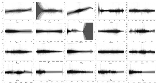
Figure 21. GAMLSS multiplot of $U_{dev}$ versus the rest of the continuous features of the main dataset.

From Figure 21 it is possible to conclude that the only interesting relationships among the available features are $U_{dev}$, $U_{COP}$ and $U_{GPS}$. Consequently, Figure 22 applies $U_{dev}$ and $U_{COP}$ as response variables and $U_{GPS}$ as explanatory variable in the GAMLSS model (6) for top and bottom graphs, respectively. The expected behavior of the scatter points of $U_{dev}$ and $U_{COP}$ is a funnel-shaped plot, starting narrow and getting wider with increasing $U_{GPS}$. However, only by looking at the scatter points it is not clear how to distinguish the shape of the funnel, if any, apart from the nonlinear relationship of $U_{dev}$ and $U_{COP}$ with $U_{GPS}$. With the centiles included in the graphs, one can compare the distributions of $U_{dev}$ and $U_{COP}$ by location.

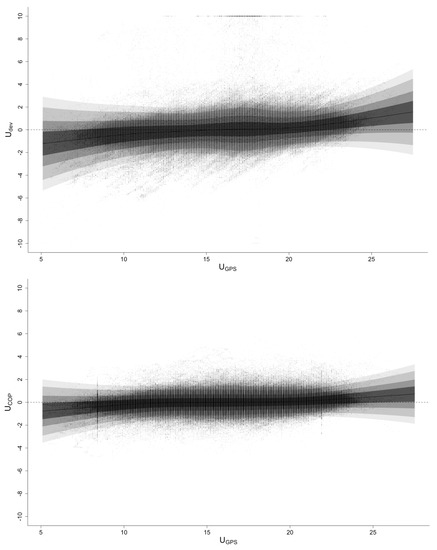
Figure 22. Centile curves using GAMLSS of $U_{dev}$ and $U_{COP}$ over $U_{GPS}$ as explanatory variable for the main dataset.

It is clear that both graphs’ medians (thick black middle line) follow the same pattern over whole range of $U_{GPS}$ which indicate a matching pattern of sea current predictions and speed measurements. However, in $U_{dev}$ there is a bigger fluctuation of the median compared to the one from $U_{COP}$. Also, the centile areas are wider in $U_{dev}$ compared to $U_{COP}$. This means that the $\sigma$ of the $U_{dev}$ distribution is always higher than that of $U_{COP}$ within the whole range of $U_{GPS}$. Consequently, one can assume that the speed sensors can capture the stream of the currents with a higher intensity than expected. Or contrariwise, one can assume that the external weather provider cannot capture the true intensity of the sea currents and how it affects a ship’s hull.

5. Summary and Conclusions

Acquiring high-accuracy speed through water (STW) measurements has been a hot topic in maritime society for many years. STW is one of the most significant signals for driving fuel consumption, costs and greenhouse gas emissions down. The transformation of the physical quantity of water mass passing down the hull of a ship to a digital signal of high accuracy is a complex procedure that ends up in measurements with error. However, fusing a large volume of high-frequency data from engine and motion sensors to evaluate and compare the STW measurements is a process towards the elimination of that error. This study attempted to simplify the identification of a highly erroneous DVL sensor based on data of Maersk Line’s fleet. The data originated from 190 container vessels, each one equipped with a continuous monitoring system. Based on measurements from GPS coordinates and compass true heading, wave data from ERA5 [28], sea regions data from IHO seas [24] and sea currents data from E.U. Copernicus Marine Service Information [27] they were merged into the main dataset, encompassing $\approx 7$ million 10-min spaced rows to be analyzed.

Essentially, the study focused on an analysis relying on two measures of the same quantity being the sea current. The one measure $U_{dev}$ ($U_{dev}=U_{GPS}-U_{DVL}$) was based on ship data, while the other measure $U_{COP}$ came as a numerical estimate (CMEMS, [27]). According to the results of the analysis, $2.47\%$ of the $U_{dev}$ distribution spans above 2 kn with a standard deviation of $0.91$ kn. On the contrary, only $0.63\%$ of the $U_{COP}$ distribution was above 2 kn with a standard deviation of $0.56$ kn. This indicates that $U_{dev}$ and $U_{COP}$ did not convey the same picture as expected. Given the defined threshold of 2 kn, one can identify a ship with a highly erroneous DVL sensor by checking its $U_{dev}$ distribution and measuring if the number of points above the threshold surpasses the fleet’s average percentage boundary of $2.47\%$. According to the data, $26\%$ of the ships of the fleet exceeds the percentage boundary.

The main dataset upon which the whole study has been-based, encompasses categorical features such as the DVL manufacturer, the sea region and the vessel class. The study showed that the DVL manufacturer was not a feature as significant as initially expected. On the other hand, vessel class proved to be an influential factor of DVL accuracy, mainly because sister ships share the same characteristics in terms of hull and voyage seaways. However, it was pinpointed that each ship should be examined separately and not as part of a class nor as part of a potential defective DVL. Concerning sea regions, it has turned out that some of them were fickler than others. Usually, the narrower and shallower seas are the ones with the highest volatility regarding sea water currents. For those regions, the STW measurements were prone to confront significant errors far from reality. Regions with high volatility such as the English Channel also affected the correlation between $U_{dev}$ and $U_{COP}$ due to the low temporal and spatial resolution of the weather data. In fact, sea region proved to be the most influential categorical feature on the STW accuracy.

The mean values of the boxplots from $U_{dev}$ distribution on some ships were either positive or negative which implies head or following currents adequately. When this happens, one can assume that a ship is a subject of bad or good voyage planning. On the other hand, checking at the $U_{COP}$ distribution of the same ships revealed that the mean values were close to zero as expected, due to the long time window of each ship. Consequently, the study affirmed that any assumption should not be-based exclusively on SOG and STW but it is recommended to incorporate the speed of the currents for confirmation.

The regression analysis showed that $U_{COP}$ was the only continuous feature correlating with $U_{dev}$. Additionally, it was spotted that the local variance of $U_{dev}$ was always higher than that of $U_{COP}$ within the whole range of GPS speed. The above implies that DVLs capture the stream of the currents with higher intensity than expected.

The availability of a monitoring tool able to determine the trustworthiness of the measured STW could be very useful to enhance both on-board and on-shore voyage data analytics. The correct knowledge of the STW is paramount for the assessment of the ship’s resistance, which in turn is a determinant factor in assessing the expected fuel and overall energy consumption during a voyage. Therefore, by improving the reliability of the STW measurement it will be possible to improve the assessment of the fuel/energy consumption. Similarly, by analyzing the STW with the propulsion power it will be possible to assess the increase in resistance, and this could lead to a more precise scheduling of hull/propeller cleaning events.

Future Work

The built dataset will be a great asset for future research and development. The first rational continuation of this study will be to create a model detecting wrong coordinate pairs from the GPS signal and replacing them with the coordinate estimates of the nearest true location. Consequently, this model will improve the weather data quality and sea regions accuracy of the dataset. Additionally, this GPS filtering model can be placed on-board before each ship’s CAMS data storage and correct the data in real time right before the coordinates are registered into the system. The above validation model will save a great number of resources from any fleet management team.

The present study has focused on exploring the marginal association between each of the features of the main dataset and $U_{dev}$. Although this exploratory approach did not reveal any significant dependencies the interpretation can be challenging if confounding factors are present. We therefore aim to supplement this analysis in future research with more sophisticated analyses based on multiple regression techniques while adjusting for error-in-variables and missing data.

An additional project that would enhance the outcome of this study would be an experiment test application where a sonar STW sensor [39] would be installed for a long period in one of the ships with tested good performing STW sensor, crossing multiple volatile sea regions (such as English Channel, Malacca Strait, Bay of Biscay, Strait of Gibraltar, Philippine sea, etc.). Then comparing $U_{dev}$, $U_{COP}$ with the new sonar-based measurement ($U_{dev-son}$), created by subtracting SOG ($U_{GPS}$) from sonar STW ($U_{SON}$) such that $U_{dev-son}=U_{SON}-U_{GPS}$, will affirm the two matching signals, revealing where the truth lies upon.

Finally, an extension of the STW estimator built on [4] would be a great step forward. Throughout that paper, it was shown that despite the few simplifying assumptions the evaluation of the designed STW estimator on the full-scale data was positive and it showed the feasibility of using a pure kinematic model to estimate a STW signal. Extending this model to a nonlinear kinetic model by discarding the simplified assumptions will be an interesting approach to drive the error further down.

References

- MAN Energy Solutions. Basic Principles of Ship Propulsion; MAN: Augsburg, Germany, 2018; Available online: www.man-es.com (accessed on 20 May 2020).
- Carlton, J. Marine Propellers and Propulsion, 4th ed.; Elsevier: Amsterdam, The Netherlands, 2019. [Google Scholar]
- Adland, R.; Cariou, P.; Wolff, F.C. Optimal ship speed and the cubic law revisited: Empirical evidence from an oil tanker fleet. Transp. Res. Part E 2020, 140, 101972. [Google Scholar] [CrossRef]
- Ikonomakis, A.; Galeazzi, R.; Dietz, J.; Holst, K.K.; Nielsen, U.D. Application of Sensor Fusion to Drive Vessel Performance. In Proceedings of the 4th Hull Performance & Insight Conference (HullPIC’19), Gubbio, Italy, 6–8 May 2019; pp. 229–241. [Google Scholar]
- Tetley, L.; Calcutt, D. Electronic Navigation Systems; Routledge: London, UK, 2007; Chapter 3; pp. 45–87. [Google Scholar]
- STT International Limited. Srd-500 Dual Axis Doppler Speed Log; Operation Manual; STT International Limited: London, UK, 1998. [Google Scholar]
- Hasselaar, T.; Fagergren, A. Speed Log Research—STW Measurement Validation Based on Performance Data MV Belgian Express; MARIN: Wageningen, The Netherlands, 2011. [Google Scholar]
- Spindel, R.; Porter, R.; Marquet, W.; Durham, J. A high-resolution pulse-Doppler underwater acoustic navigation system. IEEE J. Ocean. Eng. 1976, 1, 6–13. [Google Scholar] [CrossRef]
- Brokloff, N.A. Matrix algorithm for Doppler sonar navigation. In Proceedings of the OCEANS’94, Brest, France, 13–16 September 1994; Volume 3, p. III-378. [Google Scholar]
- Brokloff, N.A. Dead reckoning with an ADCP and current extrapolation. In Proceedings of the Oceans’ 97. MTS/IEEE Conference Proceedings, Halifax, NS, Canada, 6–9 October 1997; Volume 2, p. 1411. [Google Scholar]
- Whitcomb, L.; Yoerger, D.; Singh, H.; Mindell, D. Towards precision robotic maneuvering, survey, and manipulation in unstructured undersea environments. In Robotics Research; Springer: Berlin/Heidelberg, Germany, 1998; pp. 45–54. [Google Scholar]
- Kinsey, J.C.; Whitcomb, L.L. Preliminary field experience with the DVLNAV integrated navigation system for oceanographic submersibles. Control Eng. Pract. 2004, 12, 1541–1549. [Google Scholar] [CrossRef]
- McEwen, R.; Thomas, H.; Weber, D.; Psota, F. Performance of an AUV navigation system at Arctic latitudes. IEEE J. Ocean. Eng. 2005, 30, 443–454. [Google Scholar] [CrossRef]
- Committee, M. Final Report and Recommendations to the 24th ITTC. In Proceedings of the 24th International Towing Tank Conference, Edinburgh, UK, 4 September 2005; Volume 1, pp. 137–198.
- Kinsey, J.C.; Eustice, R.M.; Whitcomb, L.L. A survey of underwater vehicle navigation: Recent advances and new challenges. In Proceedings of the IFAC Conference of Manoeuvering and Control of Marine Craft, Lisbon, Portugal, 20–22 September 2006; Volume 88, pp. 1–12. [Google Scholar]
- ISO. ISO—ISO 19030-1:2016—Ships and Marine Technology—Measurement of Changes in Hull and Propeller Performance—Part 1: General Principles. 2016. Available online: https://www.iso.org/standard/63774.html (accessed on 20 May 2020).
- Taudien, J.Y.; Bilen, S.G. Quantifying Long-Term Accuracy of Sonar Doppler Velocity Logs. IEEE J. Ocean. Eng. 2018, 43, 764–776. [Google Scholar] [CrossRef]
- Lajic, Z.; Senteris, A.; Filippopoulos, I.; Pearson, M. Transformation of Vessel Performance System into Fault-tolerant Syste-Example of Fault Detection on Speed Log. In Proceedings of the 2019 4th International Conference on System Reliability and Safety (ICSRS), Rome, Italy, 20–22 November 2019; pp. 331–338. [Google Scholar]
- Griffiths, G.; Bradley, S.E. Correlation speed log for deep waters. Sea Technol. 1998, 39, 29–36. [Google Scholar]
- Lellouche, J.; Legalloudec, O.; Regnier, C.; Levier, B.; Greiner, E.; Drevillon, M. Quality Information Document for Global Sea Physical Analysis and Forecasting Product Global Analysis Forecast Phy 001 024; Technical Report; Copernicus Marine Service (CAMS): Luxembourg, 2016. [Google Scholar]
- Bole, A.G.; Wall, A.D.; Norris, A.; Dineley, W. Radar and ARPA Manual: Radar and Target Tracking For Professional Mariners, Yachtsmen and Users of Marine Radar; Elsevier: Amsterdam, The Netherlands, 2014; Chapter 9; pp. 407–423. [Google Scholar]
- Cenedese, C.; Gordon, A.L. Ocean Current. Encyclopædia Britannica. 2018. Available online: https://www.britannica.com/science/ocean-current (accessed on 10 March 2021).
- Lumpkin, R.; Johnson, G.C. Global ocean surface velocities from drifters: Mean, variance, El Niño–Southern Oscillation response, and seasonal cycle. J. Geophys. Res. Ocean. 2013, 118, 2992–3006. [Google Scholar] [CrossRef]
- International Hydrographic Organization; Sieger, R. Limits of Oceans and Seas in Digitized, Machine Readable Form; International Hydrographic Organization: Monaco, 2012; Available online: https://doi.pangaea.de/10.1594/PANGAEA.777976 (accessed on 22 April 2021). [CrossRef]
- International Hydrographic Organization Limits of Oceans and Seas; International Hydrographic Organization: Monegasque, Monte-Carlo, Monaco, 1953.
- Coraddu, A.; Oneto, L.; Baldi, F.; Cipollini, F.; Atlar, M.; Savio, S. Data-driven ship digital twin for estimating the speed loss caused by the marine fouling. Ocean Eng. 2019, 186. [Google Scholar] [CrossRef]
- Lellouche, J.M.; Greiner, E.; Le Galloudec, O.; Garric, G.; Regnier, C.; Drevillon, M.; Benkiran, M.; Testut, C.E.; Bourdalle-Badie, R.; Gasparin, F.; et al. Recent updates to the Copernicus Marine Service global ocean monitoring and forecasting real-time 1/12° high-resolution system. Ocean Sci. 2018, 14, 1093–1126. [Google Scholar] [CrossRef] [Green Version]
- Hersbach, H.; Bell, B.; Berrisford, P.; Biavati, G.; Horányi, A.; Muñoz Sabater, J.; Nicolas, J.; Peubey, C.; Radu, R.; Rozum, I.; et al. ERA5 Hourly Data on Single Levels from 1979 to Present, Copernicus Climate Change Service (C3S) Climate Data Store (CDS). 2018. Available online: https://cds.climate.copernicus.eu/cdsapp#!/dataset/reanalysis-era5-single-levels?tab=form (accessed on 22 April 2021). [CrossRef]
- Nielsen, U.D. Spatio-temporal variation in sea state parameters along virtual ship route paths. J. Oper. Oceanogr. 2021, 1–18. [Google Scholar] [CrossRef]
- Dalheim, Ø.Ø.; Steen, S. Preparation of In-Service Measurement Data for Ship Operation and Performance Analysis. Ocean Eng. 2020, 212, 107730. [Google Scholar] [CrossRef]
- Ikonomakis, A. The Depth Variation of Sea Currents—How Close to the Keel Is the STW Measured? 2020. Available online: https://orbit.dtu.dk/en/activities/the-depth-variation-of-sea-currents-how-close-to-the-keel-is-the- (accessed on 20 March 2021).
- Chu, P. Statistical Characteristics of the Global Surface Current Speeds Obtained From Satellite Altimetry and Scatterometer Data. IEEE J. Sel. Top. Appl. Earth Obs. Remote Sens. 2009, 2, 27–32. [Google Scholar] [CrossRef]
- Farrell, J. Aided Navigation: GPS with High Rate Sensors, 1st ed.; McGraw-Hill, Inc.: New York, NY, USA, 2008. [Google Scholar]
- Reynaud, J.; Teyssier, B.; Auffret, J.; Berné, S.; De Batist, M.; Marsset, T.; Walker, P. The offshore sedimentary cover of the English Channel and its northern and western approaches. J. Quat. Res. 2003, 18, 261–282. [Google Scholar]
- Tidetech. Tidemap. 2020. Available online: https://maps.tidetech.org/?layer=tidal_currents_english_channel&baseLayer=Topographic (accessed on 27 October 2020).
- de Winter, J.C.; Gosling, S.D.; Potter, J. Comparing the Pearson and Spearman correlation coefficients across distributions and sample sizes: A tutorial using simulations and empirical data. Psychol. Methods 2016, 21, 273. [Google Scholar] [CrossRef] [PubMed]
- Stasinopoulos, M.D.; Rigby, R.A.; Heller, G.Z.; Voudouris, V.; De Bastiani, F. Flexible Regression and Smoothing: Using GAMLSS in R; CRC Press: Boca Raton, FL, USA, 2017. [Google Scholar]
- Stasinopoulos, D.M.; Rigby, R.A. Generalized additive models for location scale and shape (GAMLSS) in R. J. Stat. Softw. 2007, 23, 1–46. [Google Scholar] [CrossRef] [Green Version]
- Gangeskar, R.; Prytz, G.; Bertelsen, V. Distributing Real-Time Measurements of Speed Through Water from Ship to Shore. In Proceedings of the 4th Hull Performance & Insight Conference (HullPIC’19), Gubbio, Italy, 6–8 May 2019; pp. 114–127. [Google Scholar]
Publisher’s Note: MDPI stays neutral with regard to jurisdictional claims in published maps and institutional affiliations. |
© 2021 by the authors. Licensee MDPI, Basel, Switzerland. This article is an open access article distributed under the terms and conditions of the Creative Commons Attribution (CC BY) license (https://creativecommons.org/licenses/by/4.0/).