A Generalized Hybrid RANSE/BEM Approach for the Analysis of Hull–Propeller Interaction in Off-Design Conditions

Abstract

During maneuvers, propellers’ operation differs from their design due to strong modification of the wake field with respect to the straight-ahead motion. The consequent modification of the loads overstresses the mechanical components of the shaftline, exacerbates propeller side effects and worsens overall efficiency. Therefore, the analysis of these situations in the early design phase is pivotal to increase the operation capabilities and safety at sea. This task relies on novel tools capable to accurately predict the complex flow field that develops past the hull and the propeller loads. Since the solution of the fully coupled problem with the rotating propeller by viscous flow solver is impractical for routine applications, hybrid approaches are a viable alternative. In this paper, an interactive RANSE/BEM methodology is presented, where the propeller is replaced by rotating body forces that map the actual loading state of the blades, allowing a fully unsteady analysis of hull–propeller interaction. The methodology is applied to the straight ahead and $8.4°$ pure drift motions of a twin screw propulsive configuration. Last, but not least, the study presents a validation study with accurate experimental data of the nominal wake field and single blade loads.

1. Introduction

Propeller performance is strongly influenced by the working conditions during the manoeuvres. Generally, in these conditions, the inflow is markedly affected by the large cross flow induced by the hull rotational motion and complex blade–wake interactions caused by flow separation and passage of coherent structures through the propeller disc. Thus, the propeller blades operate far from the optimal incidence they were designed for and develop a completely different system of loads. Extensive experimental activity by free running model tests for twin screw propulsive configurations [1] highlighted that internal and external propellers experience an asymmetric behavior characterized by increase in thrust and torque up to 100% and 60% on the external side and 60% and 40% on the internal side and the generation of radial force up to 30% of the thrust in the approach phase.

Related numerical analysis has shed light on the mechanisms that drive this asymmetric behavior of the propellers during maneuvers [2]. On the external side, the inflow resembles a pure oblique flow, and the strong propeller overloading and the generation of in-plane loads were ascribed to the increase in the tangential flow associated with the lateral motion relative to the blade sections of the propeller. On the other hand, the internal propeller is affected by complex interactions with the wake shed by the hull, which evolves with different morphology: as the rudder angle increases, the flow ranges from being characterized by coherent structures that yield strong velocity gradients, to completely vortex-dominated flow with characteristic scale comparable to the diameter of the propeller.

To further shed light on the blade/propeller interactions, a novel experimental set-up dedicated to the measurements of the single blade loads was developed and installed on a free running maneuvering model [3,4]. The measurements further stressed that the maximum thrust (torque) and bending moment developed by the single blade can be doubled with respect to the average loads on the external side during the tightest maneuver or during weak or transient maneuvering if blade/vortex interactions occur. Moreover, the fluctuations of the spindle torque were three times higher than the straight-ahead motion. The evolution of both the mean and fluctuating component of the propeller loads can consequently worsen the structural reliability of the shafting or propeller pitch mechanism [5] and amplify undesired side effects such as propeller–hull-induced pressure or noise [6] other than those that contribute to the dynamic response of the vehicle [7]. As a matter of fact, these analyses have also stressed that weak maneuvers can be as critical as the tightest ones. Moreover, due to their higher probability of occurrence during realistic conditions at sea, it is pivotal to consider these conditions starting from the early stages of the design. Since the complexity of the propeller inflow that can yield high incidences at the blade sections, standard design tools can be inadequate. Advanced Computational Fluid Dynamic techniques, based on the averaged solution of the Navier–Stokes equation, despite being feasible to pursue the direct simulation of the rotating propeller behind the hull [8,9,10], are yet impractical for day-by-day applications due to the burden of computational resources.

To overcome these limits, hybrid approaches, consisting of the interactive coupling of the viscous solver with a simplified propeller model based on potential theories have been developed. Basically, in these approaches, the propeller is replaced by body forces that are consistent with the loads calculated by the propeller solver. At increasing levels of accuracy and, hence, computational effort, the propeller can be modeled by actuator disk, blade element momentum theory ($BEMT$) or boundary element method ($BEM$). Moreover, the volume forces can be representative of the averaged behavior of the effect of the propeller over the period of revolution or describe the time-varying loading state of individual blades per cycle. The first methodology is the standard and most computationally efficient solution because the time scales relative to the propeller flow are inherently neglected. This approach has been proposed both in self-propulsion predictions and ship maneuvering [7,11,12,13]. On the other hand, the fully unsteady coupling can be pursued in cases the prediction of the propeller loads or their fluctuating character play a critical role, for example ship-dynamic- (i.e., maneuvering or motion in waves) or propeller-induced side effect analysis. In more detail, the effect of the propeller is modeled by a rotating body force distribution that mimics each blade loading during its revolution. Since the blades have to be represented specifically, the body forces are usually predicted by $BEM$ models in the context of ship propulsion [14,15,16,17], although the simpler $BEMT$ models, enhanced with a priori corrections obtained by viscous flow computations, can be a computationally cheaper alternative [18]. In this regard, a preliminary validation study showed that $BEMT$ and $BEM$ provided comparable results for the same test case studied in [2] in terms of maneuvering loads [19]. However, $BEM$ provides detailed loads, thanks to its capability to describe the pressure and load distribution on the effective geometry. Hence, it can be an attractive compromise with respect to the viscous computations with rotating propellers.

In the present work, an unsteady $RANSE$/$BEM$ hybrid methodology that models the effects of the rotating propeller is considered. The hybrid methodology, applied by means of an unsteady DES simulation of a propeller–rudder configuration has been validated against global loads exerted by the propeller [20]. The present methodology has been applied to a twin screw ship in straight-ahead motion and weak drift angle 8.4$°$ [21]. In the present paper, the work has been revised with an extensive in-depth validation process aimed to define the range of applicability of the overall numerical model and nonetheless to recognize the uncertainty propagation during the data processing in the chain by the single models. The validation process is developed in two steps. At, first the nominal wake field computed with the viscous solver for the fully appended and un-propelled hull is compared against the S–PIV measurements corresponding to the propeller plane. At the second step, the propeller loads obtained by the fully unsteady $RANS/BEM$ method are inspected in detail and compared with single blade loads measurements. The errors occurring on the blade loads, i.e., forces and moments, are related to the uncertainty of the predicted nominal wake-field through the support of the effective inflow computed by the BEM model and derived quantities. The local phenomena are then analyzed with the support of the pressure distribution on key sections over the blade revolution.

2. Theoretical Model

The proposed hybrid viscous/inviscid model was presented in [21], in which the velocity field is assumed to be the combination of two contributions: an arbitrary onset flow with velocity $\mathbf{w}$ and the velocity perturbation ${\mathbf{v}}_{{}_P}$ induced by a propeller immersed in it. Propeller flow is studied via a boundary element model for inviscid flows, while a Navier–Stokes solver is used to describe the onset flow under general viscous flow conditions. In this section, a brief description of both RANS and BEM models follows, with emphasis on the interactive procedure. For more details, the interested reader is addressed to the cited literature.

2.1. Inviscid Flow Model by BEM

Assuming an inviscid, irrotational propeller-induced flow, perturbation velocity can be described in terms of a scalar velocity potential $\phi$, ${\mathbf{v}}_{{}_P}=\nabla \phi$. Under incompressible flow assumptions, the conservation equations of mass and momentum yield to the Laplace equation for the velocity potential $\phi$, whereas the pressure p follows from the Bernoulli equation, as

$$\begin{array}{c}{\nabla }^2\phi =0\hfill \\ \frac{{\partial }^{}\phi }{\partial t^{}}+\frac{1}{2}\parallel \nabla \phi +{\mathbf{v}}_{{}_I}\parallel {}^2+\frac{p}{\rho }+g{z}_0\hfill & =& \frac{1}{2}{\parallel {\mathbf{v}}_{{}_I}\parallel }^2+\frac{p_0}{\rho }\hfill \end{array}$$

(1)

where $\rho$ is water density, $p_0$ is the free-stream pressure and $g{z}_0$ is the hydrostatic head. The inflow velocity is the superposition of the propeller angular velocity $\Omega$ and the onset flow $\mathbf{w}$, taking into account for viscosity effects and addressed by the RANS model. Quantity ${\mathbf{v}}_{{}_I}=\mathbf{w}+\Omega \times \mathbf{x}$ indicates the inflow to the propeller, while $\mathbf{x}$ represents the coordinate position in the frame of reference fixed to the rotating propeller.

The Laplace equation for $\phi$ is solved by a boundary integral representation following [22] as

$$\begin{array}{ccc}\hfill E\left(\mathbf{x}\right)\phi (\mathbf{x},t)& =& {\int }_{{\mathcal{S}}_{{}_B}}\left(\frac{{\partial }^{}\phi }{\partial n^{}}G-\phi \frac{{\partial }^{}G}{\partial n^{}}\right)d\mathcal{S}-\hfill \\ & +& {\int }_{{\mathcal{S}}_{{}_W}}\Delta {\phi }_{{}_{TE}}(t-\tau )\frac{{\partial }^{}G}{\partial n^{}}d\mathcal{S}\hfill \end{array}$$

(2)

where ${\mathcal{S}}_{{}_B}$ is the propeller surface, ${\mathcal{S}}_{{}_W}$ is the zero-thickness propeller trailing wake, t is time, $\Delta {\phi }_{{}_{TE}}$ denotes potential discontinuity shed in the wake and detached at blade trailing edge with a time delay of $\tau$ (Kutta condition). Quantities $G,{\partial }^{}G/\partial n^{}$ are unit source and dipole in the unbounded three-dimensional space. The field function $E\left(\mathbf{x}\right)$ assumes value ($E=1$) for $\mathbf{x}$ denoting a point in the flow-field and ($E=1/2$) for solid boundary surface points.

The velocity potential vanishing at infinity and the impermeability condition on the propeller surface provides boundary conditions for $\phi$. In particular, the impermeability condition $({\mathbf{v}}_{{}_P}+{\mathbf{v}}_{{}_I})·\mathbf{n}=0$ yields

$$\begin{array}{c}\hfill \frac{{\partial }^{}\phi }{\partial n^{}}=-\left(\mathbf{w}+\Omega \times \mathbf{x}\right)·\mathbf{n}\end{array}$$

(3)

where $\mathbf{n}$ is the unit normal to the surface pointing into the fluid.

The problem (1) is solved in terms of velocity potential through a linear system of equations with unknowns located on the propeller surface. The numerical solution to Equation (2) is obtained here by a low-order Boundary Element Method implemented into the PRO-INS code developed at CNR-INM (former INSEAN). The pressure distribution on the propeller blades is evaluated through the Bernoulli Equation (1).

Hydrodynamic forces are determined as

$$\begin{array}{c}\hfill \mathbf{f}=\sum _{k=1}^Z{\int }_{{\mathcal{S}}_{{}_{B_k}}}\left(-p\mathbf{n}+\tau \right)d\mathcal{S},\end{array}$$

(4)

where ${\mathcal{S}}_{{}_{B_k}}(k=1,...Z)$ denotes the surface of the k-th blade of a Z-bladed screw; $\tau$ represents the viscosity-induced tangential stress and is estimated by using expressions that are valid for flat plates in laminar and turbulent flow at same Reynolds number as blade sections.

In the following analysis, pressure and loads are made non-dimensional. In particular, the pressure distribution on the blade surface is referred to as

$$\begin{array}{c}\hfill C_P=-\frac{p-p_0}{2\rho n_0^2{D}^2}\end{array}$$

(5)

with $n_0$ indicating the propeller rate of revolution and D the propeller diameter. Force and moment components are made non-dimensional following the standard approach for the thrust and torque coefficients:

$$\begin{array}{ccc}\hfill K_{Ti}& =& \frac{T_i}{\rho n_0^2{D}^4}\hfill \\ \hfill K_{Qi}& =& \frac{Q_i}{\rho n_0^2{D}^5},i=x,y,z\hfill \end{array}$$

(6)

2.2. Viscous Flow Model by RANS

The viscous flow surrounding the propeller is evaluated by integration of the Navier–Stokes equations for unsteady incompressible flows:

$$\begin{array}{ccc}\hfill & & \nabla ·\mathbf{v}=0\hfill \\ & & \frac{{\partial }^{}\mathbf{v}}{\partial t^{}}+(\mathbf{v}·\nabla )\mathbf{v}=-\frac{1}{\rho }\nabla p+\nu {\nabla }^2\mathbf{v}+\mathbf{b}\hfill \end{array}$$

(7)

where quantity $\mathbf{b}$ denotes the source term, which indicates the propeller-induced forces derived by BEM prediction of blade loads.

The numerical algorithm to solve Equation (7) is implemented into an in-house solver based on a finite volume approach with pressure and velocity co-located at the cell center. Viscous terms are integrated by a standard second-order centered scheme, whereas for the convective and pressure terms, a third order upwind scheme is used. Turbulence effects on the Reynolds averaged flow is accounted for by means of the Spalart–Allmaras one equation model [23].

The physical time derivative in the governing equations is approximated by a second-order accurate, three-point backward finite difference formula [24]. In [25], a pseudo-time derivative is introduced in the discrete system of equations to obtain a divergence-free velocity field at every physical-time step. The scheme is formally second-order in space and time. The BEM algorithm is invoked within the pseudo-time loop with a fixed frequency chosen by numerical tests, updating the $\mathbf{b}$ term in Equation (7).

No-slip boundary conditions are enforced at solid walls. At the inlet boundary, the velocity is set to the undisturbed flow value, whereas at the outflow, the pressure gradient is supposed and the velocity is extrapolated.

The fluid domain is discretized by a system of structured, partially overlapping blocks, and a chimera algorithm is used in order to interpolate the solution among different chimera sub-grids [26,27,28].

The propeller effects in the viscous/inviscid coupling procedure are introduced with a body–force fashion. Specifically, propeller blades are not represented as solid boundaries of the computational domain and a cylindrical grid block is placed to fill the propeller region. Volume forces ${\mathbf{b}}_0$ describing propeller induction and predicted by BEM are distributed over this grid block and added as source term $\mathbf{b}$ to the right-hand side of the momentum equations.

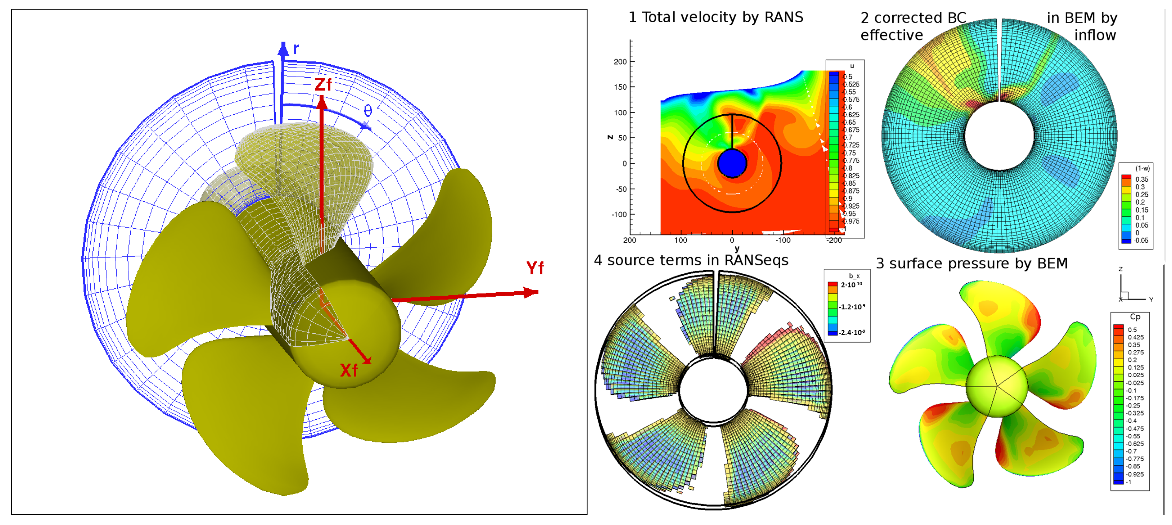
2.3. RANS/BEM Coupling

The viscous/inviscid coupling strategy presented in [21] is used here and briefly recalled. Viscous and inviscid-flow solutions are integrated through the exchange of two quantities:

• volume-forces $\mathbf{b}$, derived from the propeller hydrodynamic forces by BEM ${\mathbf{b}}_0$, are used as forcing terms of the Navier–Stokes equations;
• effective-inflow $\mathbf{w}=\mathbf{v}-{\mathbf{v}}_{{}_P}$, which is used in the BEM to impose boundary conditions on propeller surface from the estimation of the total velocity $\mathbf{v}$ by RANS.

A time-accurate approach is adopted, providing a volume force distribution according to the actual propeller position.

At each time step, elementary load contributions $(-p\mathbf{n}+\tau )$ (Equation (4)) of pressure and suction sides of each blade are summed and associated to the mean (camber) surface ${\widehat{\mathcal{S}}}_{{}_{B_k}}$. The force distribution ${\mathbf{b}}_0$ is derived from the time-dependent position of the propeller blades in the torus cells marked by the position of the ${\widehat{\mathcal{S}}}_{{}_{B_k}}$. The Dirac distribution is mitigated along propeller axis x adopting a normalized Gaussian distribution $\xi =\xi \left(x\right)$. The resulting source terms of Equation (7) with respect to the rotating frame of reference in Figure 1 (left) are

$$\begin{array}{c}\hfill \int \mathbf{b}(x,r,\theta ,t)dx={\mathbf{b}}_0(r,\theta ,t)\int \xi \left(x\right)dx\end{array}$$

(8)

In the present study, the distribution is set such that the integral in the right-hand side of Equation (8) is 0.99 for extremes exceeding 30% of the nominal propeller width.

The viscous and potential-flow solutions are achieved within the inner iteration of the dual-stepping procedure, used to reach a solenoidal solution of Navier–Stokes equations.

At each step of the pseudo-time loop, the effective velocity distribution $\mathbf{w}$ is evaluated by BEM, on the basis of the total velocity $\mathbf{v}$ by RANS and the perturbation velocity ${\mathbf{v}}_{{}_P}$ by BEM calculated in the preceding step. The boundary conditions by Equation (3) are imposed, and BEM equations are solved for $\phi$. From the volume force distribution ${\mathbf{b}}_0$, source terms $\mathbf{b}$ of the RANS Equation (7) are derived. The solution to such equations yields a new estimate of the total velocity $\mathbf{v}$. The body force distribution ${\mathbf{b}}_0$ follows the BEM call for a fixed frequency in the pseudo-time loop in order to increase convergence history.

A time-marching solution is achieved with BEM and RANS parameters synchronized to the propeller rotation.

The first BEM solution is obtained by marching in time for a number of revolutions in order to achieve a correct description of transient flow contributions of the trailing wake (Equation (2)) while preserving the synchronization. As already mentioned, the BEM used here describes an isolated propeller, and hence no contribution of the hull surface is explicitely given in Equation (2). The presence of the hull in the potential flow solution is taken into account by suitable boundary conditions based on the effective inflow $\mathbf{w}$ calculated by Equation (7). The viscous flow $\mathbf{v}$ is obtained by solving the unsteady RANS equations of the hull-fitted mesh including the propeller perturbation via source terms.

The interactive procedure steps dedicated to the velocity prediction by RANS, the correction of the BEM boundary conditions from the effective inflow, the BEM prediction of the blade pressure distribution and the body–force distribution in the torus block are sketched in Figure 1 (right).

An approximated evaluation of the effective inflow $\mathbf{w}$ is based on velocity contributions $\mathbf{v}$ and $\nabla \phi$ calculated at the torus inlet section instead of the actual propeller surface.

3. Case Study and Experimental Setup

Tests of a ship model operating in straight-ahead and steady-drift conditions, with and without the propeller action, have been reproduced by means of hybrid RANS/BEM and full RANS simulations.

Measurements were collected during a dedicated towing-tank oblique towing tests in calm water [29,30]. The case study is represented by a propelled and un-propelled ship model, for given advance speed, hull displacement and propeller rate of revolution.

Table 1. Ship and propeller models: main characteristics.

Parameter	Symbol	Model Scale
Block coefficient	$C_B$	0.49
Drift angle	$\beta$	$0;8.4°$
Speed	${\mathbf{F}}_{\mathbf{N}}$	0.26
Pitch to diameter ratio	P/D	1.45
Hub diameter ratio	${\mathbf{r}}_{\mathbf{h}}/\mathbf{R}$	0.37
Prop.s rotation	-	inward
Advance coefficient	J	1.116

summarizes the main geometric data of the hull and propeller models and test conditions. Hull model without rudders are used in order to improve the S-PIV measurements behind the propeller disc.

Particle Image Velocimetry measurements in towing-tanks usually require ad hoc solutions to address the need to protect electronic equipment from water. Pioneering works in this field [31] rely upon underwater probe systems to address this issue. In this work, a novel approach to implement a stereoscopic PIV (stereo-PIV) system is adopted, based on the use of borescopes as optical element rather than standard objectives.

The stereo-PIV system, as shown in Figure 2, consists of two TSI Powerview 8 MP cameras with a resolution of $3320\times 2496$ pixels. The laser used is a 532 nm wavelength Evergreen Nd:YAG unit, max pulse energy 200 mj, repetition rate 15 Hz.

The two cameras face the same side of the acquisition plane and are located at $R=800$ mm away from the acquisition plane at an angle of, respectively, ${\alpha }_A=50°$ and ${\alpha }_B=80°$. Measurements are carried out without the propeller, and the acquisition plane is located approximately 1 mm downstream of the starboard propeller hub. The area where the full three-component velocity field is measured has a size of 430 mm × 260 mm and is centered on the propeller’s hub.

For each test condition, a set of 400 image pairs was acquired with an acquisition frequency of 3 Hz. This ensured that samples are uncorrelated and statistical convergence of the first and second order statistics is obtained. The rationale underlying the use of borescopes as a component of a PIV system lies in the increased flexibility that this tool provides in terms of measurement region accessibility, as well as reduced intrusivity in the region of interest. Vector fields are calculated with TSI Insight 4G commercial software. It implements an iterative multi-pass, multi-grid, image deformation scheme with window-offset (see [32]). Optimal windows sub-grid resolution was set to $128\times 128$ pixels for the first pass and $64\times 64$ pixels for the second and final passes. The resulting vector grid spacing is 32 pixels (a sub-window overlap of 50% was set), which corresponds to approximately 3 mm. Upon calibration with a four-plane target, the full three-component velocity field is obtained. The image geometrical deformation, caused by the short focal distance featured by the borescope lenses, and the reduced amount of light entering the device represent the major drawback of the present experimental technique. Dedicated post-processing activity is needed to account for the image deformation. Uncertainty of measurements is assessed, taking into account both bi-dimensional cross-correlation error and stereo reconstruction error as described in [29].

The resulting uncertainty, expressed as the root-mean-square of particle displacement normalized by the free-stream velocity, $\frac{RMS\left(\mathbf{V}\right)}{\left|\mathbf{W}\right|}=(3.1;1.7;0.8)\%$, was evaluated for each component of the frame of reference shown in Figure 1.

The experimental propeller loads were obtained by a novel setup designed specifically for the measurements of the single blade loads [33] and extensively tested for free running [3,4,29] and captive model tests. In particular, the starboard propeller was completely re-designed to house a six-component transducer constrained at the root of a blade, and the propulsive line was modified in order to allow the transfer of signals inside the hull. In order to obtain the total loads, the blade measurements were converted in the hub frame, repeated and shifted according to the angular position of the blades and then summed.

4. Numerical Setup

The computational mesh built around the complete hull model was adopted for the drift motion $\beta =8.4°$, whereas, thanks to the symmetry of the geometry and the flow, only the half part was considered for the ship moving in the straight-ahead condition, $\beta =0°$. The RANS computational mesh consists of a total of 37 M hexahedral cells subdivided into 360 structured adjacent and partially overlapped blocks. A total of 23.1 M cells were dedicated to the bare hull, 6.2 to the shaft axis and relative strut supports, 5.6 M to the appendages (bilge keels, fore and aft antiroll fins), 0.8 M to the torus blocks and 1.5 M to the background. The hull model is placed across the origin, whereas the background extends from 2.3 $L_{PP}$ upstream to 3.3 $L_{PP}$ downstream. The remaining boundaries are placed 2.1 $L_{PP}$ far from the origin. Figure 3 shows details of the numerical grid at the wall of the hull and appendages. The BEM simulations were performed with a surface mesh built around the propeller blades and hub. A total of 6.7 K quadrilateral panels are considered. Each blade was discretized by $48\times 24$ panels along the chordwise and radial directions, whereas each hub sector mesh consists of $30\times 47$ along the azimuthal and longitudinal directions. The exchange quantities used in the interactive procedure (i.e., the body-forces ${\mathbf{b}}_{\mathbf{0}}$ and the total velocity components $\mathbf{u}$) were evaluated on a polar grid $40\times 128$ along the radial and azimuthal directions corresponding to a torus axial section. The hybrid model, in the present version, allows for a torus disc with a straight inner section. In order to preserve the radial extension of the blade, the physical shaft model, hosting the pitch-control mechanism, was straightened to build a computational mesh compatible with the propeller disc; see bottom of Figure 3. As the reader can verify in the following sections, the error introduced is limited to a non-realistic local flow-field at the inner radii (0.3r/R), whereas the body forces there are negligible. A further improvement in the model is scheduled to allow for a generalized shaped torus inner surface.

5. Validation Results

In the present section, results of the simulations performed to address the hydrodynamics of the ship in straight-ahead and in drift motion are presented. Results of the un-propelled hull are shown in terms of velocity field at the transverse plane in the propeller region, starboard side, by PIV measurements and hybrid RANS/BEM predictions (Figure 4, Figure 5 and Figure 6), in case of straight-ahead motion. In the following, non-dimensional velocity components with respect to the upstream velocity are shown.

The time-varying loads of a reference blade were predicted in the case of the propellers in behind-hull conditions (Figure 7) and compared to the measurements. The subscripts T and Q refer, respectively, to the forces and moments, according to thrust and torque coefficient definitions given in (6). Results of the hull in drift motion are similarly shown in Figure 8, Figure 9, Figure 10 and Figure 11 in terms of velocity components and in Figure 12 and Figure 13 in terms of load components.

In the present analysis, a polar frame $\left(O{x}_{{}_F}r\theta \right)$ is considered, centered on the propeller shaft (Figure 1). In particular, the axial direction points downstream, the azimuthal position $\theta$ increases clockwise as seen from the aft with the reference position at the $12 o^{’}clock$, whereas the radial velocity is positive outward.

5.1. Straight-Ahead ($\beta =0°$) Motion

The present methodology is validated by steps. The nominal wake-field at the transverse plane in the propeller region, starboard side, of the un-propelled hull is first investigated. S-PIV measurements and RANS predictions are shown in Figure 4.

Numerical prediction of the flow field are in good agreement with measured data. Coherent structures are captured, whereas main differences can be related to a limited diffusion rate in the field of the hull boundary layer addressed by the present model. A higher velocity defect induced by coherent structures detached from the skeg is found in the top left quadrant of the figure, as well as the persisting wake of the shaft brackets in the middle top part. Moreover, a persisting vortical structure induced by the fore stabilizer fin is predicted in the top right part of Figure 4. Similar results are obtained for the transverse components and are not shown here. A detailed comparison between predicted and measured velocity was performed on key radial sections. Results in terms of axial, tangential and radial components are shown in Figure 5 and Figure 6.

Differences highlighted in the comparison of the countour map of the axial velocity components reveal here an averaged error up to $5\%$ but a shift of about $20$, which deserves further investigation. The larger straight shaft used in the simulations instead of the real shaped hub may explain the disagreement at lower radii (Figure 3). The numerical model predicts a narrower region with a higher velocity defect at $r/R=0.30$, when the nominal propeller boss ratio is $R_H/R=0.29$. The comparison of the tangential and radial velocity components reveal differences concentrated in the region of the shaft brackets and, for the latter, in the bottom region, confirming the overprediction of the velocity defect past the hull.

Figure 7 reports the hybrid RANS/BEM predictions and experimental measurements of the time-varying loads of the reference blade. In general, the mean and the amplitude of the fluctuation are in good agreement with the experiments. Differences are amplified in correspondence with the peak at $\theta$∼$-40°$, due to overprediction of the velocity defect. This discrepancy affects in particular the bending moment $K_{Qy}$ and the spindle torque $K_{Qz}$. The negative peak of the spindle torque is consistent with the overprediction of thrust according to the behavior of this component, with blade loading described in [3].

5.2. Steady-Drift ($\beta =8.4°$) Motion

In the present section, the comparison of the predicted nominal wake and propeller loads for both the portside and the starboard side are shown when the drift angle is $8.4°$. Results for the nominal wake are shown in terms of velocity field on the transverse plane in the propeller region, by S-PIV measurements (Figure 8) and by RANS predictions (Figure 9). It has to be noted that for the external propeller (portside), the comparison of the calculated and measured inflow field is only qualitative, because the closest PIV measurements to the actual case refer to the drift angle of $\beta =13.4°$. In the present case, a defined vortical structure is apparent in the top left side of the propeller disc region, originating from flow detachment at the skeg on the starboard (leeward side). On the port side (windward side), the velocity field is characterized by the leeward deflection of the wake.

In particular, the velocity defect past the inner bracket and the propeller shaft (about $\theta$∼$90$) is evident. A good qualitative agreement between numerical prediction and experimental data is achieved, except a stronger trace of coherent structures is predicted on the leeward side.

Predicted and measured velocity components are directly compared on the main radial sections. Results in terms of axial, tangential and radial components are shown in Figure 10 and Figure 11. In particular, the left column deals with the portside propeller and the right with the starboard propeller.

Numerical and experimental data agree both in magnitude and in phase for the starboard propeller. Disagreement is recognised at lower radii and can be explained by geometry differences in correspondence with the previously mentioned hub. The trend of the flow field predictions at the portside propeller has been confirmed by comparison with experimental data for a different drift angle configuration (13.4$°$ instead of the actual 8.4$°$).

The time-varying loads of the reference blade are predicted in the case of propellers operating behind hull conditions, Figure 12 and Figure 13, and compared to the three-axis measurements of the blade loads for the port and starboard propeller. A detailed agreement is obtained for all components. In particular, the agreement with the measurements is satisfactory in terms of mean and amplitude of the fluctuation.

The evolution of the loads is completely different for the two propellers: in contrast to the mean values that experience a similar magnitude, with the exception of the spindle torque, the unsteady contribution is stronger for the starboard propeller as a consequence of the amplification of the interaction with the wake of the hull. On the port propeller (windward side), the blade loading increases in the lower half of the disk (i.e., $-180°<\theta <-90°$ and $90°<\theta <180°$). On the starboard propeller, the blade loads increase during the descending motion of the blade, in particular for $-60°<\theta <-90°$, due to the interaction with the vortical structure detached from the skeg. Local discrepancies arise at about $\theta$∼$20$, i.e., past the outer bracket, where the wake is deflected by the cross flow induced by oblique towing. Differences are apparent for $K_{QX}$ and for the bending moment $K_{QY}$. Once the predicted nominal wake shows a fluctuating trend around the measured one, the overall good agreement on thrust and side force, $K_{TX}$ and $K_{TY}$, can reasonably coexist with discrepancies in moments $K_{QY}$, $K_{QX}$, which are influenced also by local phenomena represented by the position of application of the pressure field on the blade surface.

The global loads generated by each blade can be more deeply analyzed through the pressure distribution on the blade surface as defined in (5). The instantaneous pressure distribution is shown in Figure 14, in case of straight-ahead and drift motion for the port and starboard propellers (face side).

To gain a further insight into the behavior of the blade, the blade loading was also inspected in terms of pressure distribution at representative radial sections at $r/R$ = 0.43 and 0.7 and related to the characteristics of the effective wake (shown in Figure 15 and Figure 16 and in terms of axial and tangential velocity, respectively). Moreover, Figure 17 shows the distribution of the effective angle of attack over the inlet of the actuator disk.

The incidence angle was calculated on the basis of the total velocity field at the inlet section of the actuator disc for the starboard side propeller. In the figures, the blades are numbered following the sense of rotation of the propeller starting from the top. In particular, dealing with the left-handed starboard propeller, the pressure distribution for the Z1 blade is shown in Figure 18, denoted by $\theta =-0.42°$.

In the figure, the dotted lines refer to the pressure side and lines to the suction side. The other blades, from the Z2 up to the Z5, following an anti clockwise numbering, are denoted, respectively, by $\theta =(-114°,-174°,+102°,+30°)$. The loading of the blades is consistent with the evolution of the single blade load measurements reported in previous figures.

In straight-ahead motion, the blade is overloaded during the downstroke motion ($-180°<\theta <0°$) because the velocity defect is stronger and the tangential velocity, upwards oriented, acts to increase the tangential velocity relative to the foil. As a result, in this sector, the incidence angle is higher. On the contrary, during the upstroke motion, the blade rotates in a region less affected by the hull wake, and hence, the loads drop.

In steady-drift motion, the propellers show an asymmetric behavior. The windward propeller (left panel at the bottom of in Figure 14) is more overloaded during the passage past the shaft and in the lower half of the disk. In the former case, the overloading of the blade must be ascribed to the interaction with the wake of the hull (see Figure 9). On the other hand, in the lower half of the disk, the overloading is associated with the lateral flow induced by the motion that increases the onset tangential velocity to the blade sections and thus the incidence angle (see Figure 17). During the upstroke phase of the cycle, the blade loading weakens because the axial incidence angle decreases due to increased axial velocity. The pressure distribution at the two representative sections confirm this trend. It is also interesting to observe the fact that the outer section of the blade Z4 experiences a reversal flow at the leading edge.

A completely different blade loading characterizes the leeward propeller at the starboard side. The blade is strongly loaded in position Z1 and Z5, whereas the loading drops in the remaining interval of the cycle. In more detail, at Z1, the overloading of the blade is mainly associated with the interaction with the vortex detached from the skeg that impinges the propeller disc inducing upward-directed velocities. As evidenced in Figure 9 and Figure 15, this structure causes a reduction in the axial velocity and, being counterclockwise (i.e., the same direction of rotation of the blade), increases the tangential velocity acting on the blade sections. As a consequence, the blade angle of attack (see Figure 17 on the right panel) and, in turn, the load suddenly increase, according to the coherent nature of the perturbation induced by the vortex in a limited region.

It is worth noting that close to the hub, the map of the incidence angle has been removed where the angle of attack exceeds the indicative value of 12$°$, defined as critical for the BEM solver to provide reliable results, since nonlinear lift mechanisms that can arise cannot be modeled without suitable corrective models. Then, at position Z2–Z4, the blade loading drops by the cross flow induced by the motion that weakens the tangential velocity relative to the sections. Further, blade loads at Z5 are increased by the passage across the wake shed past hull and inner bracket. Moreover, the cross flow plays an opposite role with respect to the blade passage in the lower half of the disk.

The distribution of pressure coefficient reveals that, where the blade interacts with the cross-flow, the load is slightly stronger than the strongest one developed on the external side (at position Z3). The stronger weakening of $C_P$ from Z3 to Z4 is ascribed to the small velocity defect. At Z5, the pressure rises again as a consequence of the impingement with the wake of the outer bracket. These effects on the pressure distributions are directly related to the high fluctuations recognized by the blade loading. Finally, it is interesting to observe that the leading edge of the blade is impinged at negative angle of attack during the under-loading phase of the blade, clearly evidenced by the negative values on the face of the blade in Figure 14. This behavior is mainly associated with the reduction of the tangential flow relative to the foil induced by the motion.

6. Conclusions

In the present paper, a preliminary validation of a hybrid RANS/BEM solver for the hydrodynamic analysis of a ship in prescribed motion has been presented. The problem is approached by fully unsteady hydrodynamic analyses through a hybrid computational methodology that consists of the interactive coupling between a RANSE solver for the evaluation of the nominal wake and a BEM propeller model for modeling the effect of the propeller on the flow (and the loads). The basic feature of the present methodology is that the propeller effects are resolved during the cycle; i.e., body forces are properly distributed in correspondence of the blades and evolve according to the instantaneous wake field and position of the blades. The methodology has been applied to a twin-screw model in straight-ahead condition and at a moderate drift angle. The methodology has been validated with ad hoc stereo–PIV measurements of the nominal wake field in correspondence with the propeller plane, validating the viscous solver, and single blade loads to validate the coupled RANSE/BEM procedure.

The results were in very good agreement with the experiments. Differences in the nominal wake were detected and can be associated with the grid and turbulence model adopted and geometrical difference in correspondence with the hub. The prediction of the propeller loads, in terms of mean value and absolute fluctuation, was correctly captured for all the components, while localized errors were consistent with related discrepancy of the wake field.

This numerical methodology allowed gaining a deeper insight into the hull–propeller interaction: in fact, the resolution of the pressure field on the blades highlighted the complex behavior of the blades, in which, during a period, can exceed critical stall angle or flow reversal in correspondence with the leading edge. These conditions are realistic and have a higher probability of occurrence (given the rather small drift angle) and need to account for a safer structural strength of the blade or pitch mechanisms (in case of controllable pitch-propulsive configuration) to mitigate undesired side effects, such as pressure pulses or noise. From this point of view, the methodology is particularly appealing for propeller design, since the $BEM$ description remarkably simplifies the grid treatment in parametric analysis.

A complete validation of the approach is in progress for a broad set of incidence angles ranging from small to tight maneuvering conditions.

References

1. Ortolani, F.; Mauro, S.; Dubbioso, G. Investigation of the radial bearing force developed during actual ship operations. Part 1: Straight ahead sailing and turning maneuvers. Ocean Eng. 2015, 94, 67–87. [Google Scholar] [CrossRef]
2. Dubbioso, G.; Muscari, R.; Ortolani, F.; Di Mascio, A. Analysis of propeller bearing loads by CFD. Part I: Straight ahead and steady turning maneuvers. Ocean Eng. 2017, 130, 241–259. [Google Scholar] [CrossRef]
3. Ortolani, F.; Dubbioso, G. Experimental investigation of blade and propeller loads: Straight ahead motion. Appl. Ocean. Res. 2019, 87, 111–129. [Google Scholar] [CrossRef]
4. Ortolani, F.; Dubbioso, G. Experimental investigation of blade and propeller loads: Steady turning motion. Appl. Ocean Res. 2019, 91, 101874. [Google Scholar] [CrossRef]
5. Dubbioso, G.; Ortolani, F. Analysis of fretting inception for marine propeller by single blade loads measurement in realistic operating conditions. Straight ahead and turning circle maneuver. Mar. Struct. 2020, 71, 102720. [Google Scholar] [CrossRef]
6. Dubbioso, G.; Muscari, R.; Ortolani, F.; Di Mascio, A. Numerical Analaysis of Marine Propellers Low Frequency Noise during Maneuvering. Appl. Ocean Res. 2020, 71, 399–419. [Google Scholar]
7. Broglia, R.; Dubbioso, G.; Durante, D.; Di Mascio, A. Simulation of Turning Circle by CFD: Analysis of different propeller models and their effect on manoeuvering prediction. Appl. Ocean Res. 2013, 39, 1–10. [Google Scholar] [CrossRef]
8. Mofidi, A.; Carrica, P.M. Simulations of zigzag maneuvers for a container ship with direct moving rudder and propeller. Comput. Fluids 2014, 96, 191–203. [Google Scholar] [CrossRef]
9. Castro, A.M.; Carrica, P.M.; Stern, F. Full scale self-propulsion computations using discretized propeller for the KRISO container ship KCS. Comput. Fluids 2011, 51, 35–47. [Google Scholar] [CrossRef]
10. Muscari, R.; Felli, M.; Di Mascio, A. Analysis of the Flow Past a Fully Appended Hull with Propellers by Computational and Experimental Fluid Dynamics. J. Fluids Eng. 2011, 133, 061104. [Google Scholar] [CrossRef]
11. Lee, S.; Chen, H. The Influence of Propeller/Hull Interaction on Propeller Induced Cavitating Pressure. In Proceedings of the 15th International Offshore and Polar Engineering Conference, ISOPE 2005, Seoul, Korea, 19–24 June 2005. [Google Scholar]
12. Gaggero, S.; Villa, D.; Viviani, M. An extensive analysis of numerical ship self-propulsion prediction via a coupled BEM/RANS approach. Appl. Ocean Res. 2017, 66, 55–78. [Google Scholar] [CrossRef]
13. Martin, J.; Thad, M.; Carrica, P.M. Submarine Maneuvers Using Direct Overset Simulation of Appendages and Propeller and Coupled CFD/Potential Flow Propeller Solver. J. Ship Res. 2015, 59, 1–21. [Google Scholar] [CrossRef]
14. Greve, M.; Wockner-Kluwe, K.; Abdel-Maksoud, M.; Rung, T. Viscous-Inviscid Coupling Methods for Advanced Marine Propeller Applications. Int. J. Rotat. Mach. 2012. [Google Scholar] [CrossRef] [Green Version]
15. Berger, S.; Scharf, M.; Gottsche, U.; Neitzel, J.; Angerbauer, R.; Abdel-Maksoud, M. Numerical Simulation of Propeller-Rudder Interaction for Non-Cavitating and Cavitating Flows Using Different Approaches. In Proceedings of the 4th International Symposium on Marine Propulsion, SMP’15, Austin, TX, USA, 31 May–4 June 2015. [Google Scholar]
16. Rijpkema, D.; Starke, B.; Bosschers, J. Numerical simulation of propeller-hull interaction and of the effective wake field using a hybrid RANS-BEM approach. In Proceedings of the 3rd International Symposium on Marine Propulsion, SMP’13, Lauceston, Australia, 5–7 May 2013. [Google Scholar]
17. Salvatore, F.; Calcagni, D.; Muscari, R.; Broglia, R. A generalised fully unsteady hybrid RANS/BEM model for marine propeller flow simulations. In Proceedings of the VI International Conference on Computational Methods in Marine Engineering, MARINE 2015, Rome, Italy, 15–17 June 2015; pp. 613–626. [Google Scholar]
18. Koncoski, J.; Paterson, E.; Zierke, W. A Blade-Element Model of Propeller Unsteady Forces for Computational Fluid Dynamics Simulations. In Proceedings of the International Conference on Developments in Marine CFD 2011, London, UK, 22–23 March 2011. [Google Scholar]
19. Gaggero, S.; Dubbioso, G.; Villa, D.; Muscari, R.; Viviani, M. Propeller modeling approaches for off–design operative conditions. Ocean Eng. 2019, 178, 283–305. [Google Scholar] [CrossRef]
20. Calcagni, D.; Salvatore, F.; Dubbioso, G.; Muscari, R. A generalised unsteady hybrid des/bem methodology applied to propeller-rudder flow simulation. In Proceedings of the VII International Conference on Computational Methods in Marine Engineering, MARINE 2017, Nantes, France, 15–17 May 2017; pp. 377–392. [Google Scholar]
21. Calcagni, D.; Capone, A.; Ortolani, F.; Broglia, R.; Dubbioso, G.; Pereira, F.; Salvatore, F.; Di Felice, F. A generalised hybrid RANSE/BEM approach for unsteady flow effects in hull/propeller interaction. In Proceedings of the 6th International Symposium on Marine Propulsion, SMP’19, Rome, Italy, 26–30 May 2019. [Google Scholar]
22. Morino, L. Boundary Integral Equations in Aerodynamics. Appl. Mech. Rev. 1993, 46, 445–466. [Google Scholar] [CrossRef]
23. Spalart, P. Detached-Eddy Simulation. Annu. Rev. Fluid Mech. 2009, 41, 181–202. [Google Scholar] [CrossRef]
24. Di Mascio, A.; Broglia, R.; Muscari, R.; Dattola, R. Unsteady RANS Simulation of a Manoeuvring Ship Hull. In Proceedings of the 25th ONR Symposium on Naval Hydrodynamics, St. John’s, NL, Canada, 8–13 August 2004. [Google Scholar]
25. Merkle, C.; Athvale, M. Time-accurate Unsteady Compressible Flow Algorithms Based on Artificial Compressibility. AIAA Pap. 1987, 87, 1137. [Google Scholar]
26. Muscari, R.; Di Mascio, A. Simulation of the flow around complex hull geometries by an overlapping grid approach. In Proceedings of the 5th Osaka Colloquium on Advanced Research on Ship Viscous Flow and Hull Form Design by EFD and CFD Approaches, Osaka, Japan, 14–15 March 2005. [Google Scholar]
27. Muscari, R.; Broglia, R.; Di Mascio, A. An overlapping grids approach for moving bodies problems. In Proceedings of the 16th International Offshore and Polar Engineering Conference, ISOPE 2006, San Francisco, CA, USA, 28 May–2 June 2006. [Google Scholar]
28. Zaghi, S.; Di Mascio, A.; Broglia, R.; Muscari, R. Application of dynamic overlapping grids to the simulation of the flow around a fully-appended submarine. Math. Comput. Simul. 2014, 116, 75–88. [Google Scholar] [CrossRef]
29. Ortolani, F.; Capone, A.; Dubbioso, G.; Pereira, F.A.; Maiocchi, A.; Di Felice, F. Propeller performance on a model ship in straight and steady drift motions from single blade loads and flow field measurements. Ocean Eng. 2020, 197, 106881. [Google Scholar] [CrossRef]
30. Capone, A.; Alves Pereira, F.; Maiocchi, A.; Di Felice, F. Analysis of the hull wake of a twin-screw ship in steady drift by Borescope Stereo Particle Image Velocimetry. Appl. Ocean Res. 2019, 92, 101914. [Google Scholar] [CrossRef]
31. Pereira, F.; Costa, T.; Felli, M.; Calcagno, G.; Di Felice, F. A versatile fully submersible stereo-PIV probe for tow tank applications. In Proceedings of the ASME/JSME 2003 4th Joint Fluids Summer Engineering Conference, FEDSM 2003, Honolulu, HI, USA, 6–10 July 2003; American Society of Mechanical Engineers: New York, NY, USA, 2003; pp. 101–106. [Google Scholar]
32. Scarano, F. Iterative image deformation methods in PIV. Meas. Sci. Technol. 2001, 13, R1. [Google Scholar] [CrossRef]
33. Ortolani, F.; Dubbioso, G. In-plane and single blade loads measurement setups for propeller performance assessment during free running and captive model tests. Ocean Eng. 2020, 217, 107928. [Google Scholar] [CrossRef]
Figure 1. (Left) Cylindrical frame of reference ( x , θ , r ) and Cartesian fixed frame of reference ( O x F y F z F ) used by the interactive procedure to exchange data. (Right) RANS/BEM interacting procedure.
Jmse 09 00482 g001
Figure 2. Model hull. (Top and center) towing tank and borescopic SPIV set-up. (Bottom) Multi-axial loads transducer
Jmse 09 00482 g002
Figure 3. Model hull. (Top) Hull computational mesh. (Bottom) sketch of the computational mesh in the propeller region.
Jmse 09 00482 g003aJmse 09 00482 g003b
Figure 4. Nominal wake of the model hull in straight-ahead motion: axial velocity component at the starboard side close to the propeller shaft end (position in mm). (Left) stereo-PIV measurements. (Right) RANS computations.
Jmse 09 00482 g004
Figure 5. Nominal wake of the model hull in straight-ahead motion: axial velocity components by PIV (red plots) and RANS (blue plots) at radial sections ( r / R = 0.3 ; 0.5 ; 0.70 ; 0.95 from left to right, top to bottom).
Jmse 09 00482 g005
Figure 6. Nominal wake of the model hull in straight-ahead motion: tangential (left) and radial (right) velocity components by PIV (red plots) and RANS (blue plots) at r / R = 0.70 radial section.
Jmse 09 00482 g006
Figure 7. Propulsive performances of the model hull in ahead motion at zero drift angle, J = 1.12. Single blade contribution to thrust, torque and spindle moment coefficients (left) and to the transverse force and bending moment (right) coefficients.
Jmse 09 00482 g007
Figure 8. Nominal wake of the model hull without rudders in steady drift motion: Stereo-PIV measurements of the axial velocity component on the transverse plane close to the propeller shaft end. (Left): portside. (Right): starboard.
Jmse 09 00482 g008
Figure 9. Nominal wake of the model hull without rudders in steady drift motion: RANS computations of the axial velocity component on the transverse plane close to the propeller shaft end. (Left) portside. (Right) starboard.
Jmse 09 00482 g009
Figure 10. Nominal wake of the model hull in steady drift motion, starboard: axial velocity components by PIV (red plots) and RANS (blue plots) at key radial sections ( r / R = 0.3 ; 0.5 ; 0.70 ; 0.95 from top to bottom). (Left) portside propeller. (Right) starboard propeller.
Jmse 09 00482 g010
Figure 11. Nominal wake of the model hull in steady drift motion. Tangential (top) and radial (bottom) velocity component at r / R = 0.70 radial section. (Left) portside propeller. (Right) starboard propeller.
Jmse 09 00482 g011
Figure 12. Propulsive performances of the model hull in ahead motion at 8.4 ° drift angle, J = 1.12: single blade contribution to thrust, torque and spindle moment coefficients. (Left) portside propeller. (Right) starboard propeller.
Jmse 09 00482 g012
Figure 13. Propulsive performances of the model hull in ahead motion at 8.4 ° drift angle, J = 1.12: single blade contribution to tangential force coefficient and moment. (Left) portside propeller. (Right) starboard propeller.
Jmse 09 00482 g013
Figure 14. Propulsive performances of the model hull, J = 1.12: pressure distribution on face sides. (Top) 0 ° drift angle; (Bottom) 8.4 ° drift angle, portside propeller (left), starboard propeller (right).
Jmse 09 00482 g014
Figure 15. Propulsive performances of the model hull in steady drift motion at 8.4 ° , J = 1.12: axial velocity defect at the actuator disc inlet section. (Left): portside propeller. (Right): starboard propeller.
Jmse 09 00482 g015
Figure 16. Propulsive performances of the model hull in steady drift motion at 8.4 ° , J = 1.12: in-plane velocity component through vectors at the actuator disc inlet section. (Left): portside propeller. (Right): starboard propeller.
Jmse 09 00482 g016
Figure 17. Propulsive performances of the model hull in steady drift motion at 8.4 ° , J = 1.12: incidence angle of attack at the starboard actuator disc inlet section. (Left): portside propeller. (Right): starboard propeller.
Jmse 09 00482 g017
Figure 18. Propulsive performances of the model hull in steady drift motion at 8.4 ° , J = 1.12: pressure distribution at starboard propeller sections r / R = 0.43 and 0.7. From top to bottom: propeller blade. (Left) portside propeller. (Right) starboard propeller.
Jmse 09 00482 g018aJmse 09 00482 g018b