
A Comparative Investigation of Prevalent Hydrodynamic Modelling Approaches for Floating Offshore Wind Turbine Foundations: A TetraSpar Case Study


Abstract
:1. Introduction
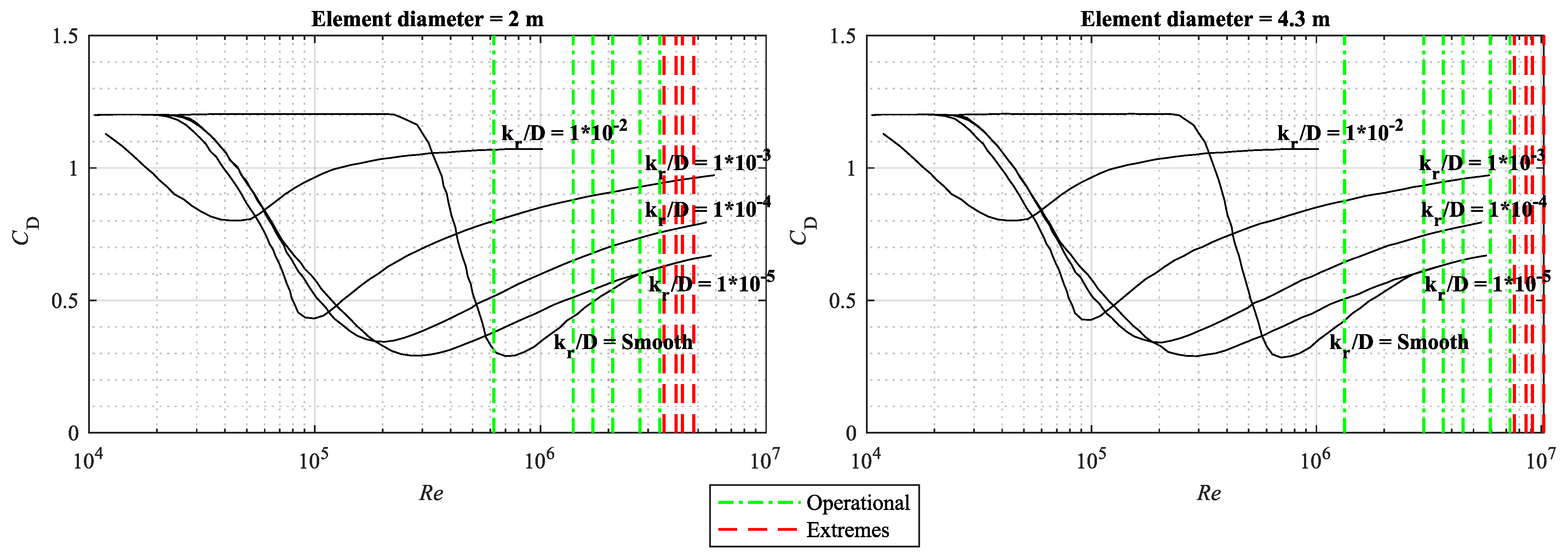
2. Methodology
2.1. Time Domain Solver: The OrcaFlex Software Package
2.2. Morison Approach
2.3. Boundary Element Method (BEM) Approach
2.4. Hybrid Modelling
2.4.1. Model Comparison
2.5. Comparing the Modelling Approaches
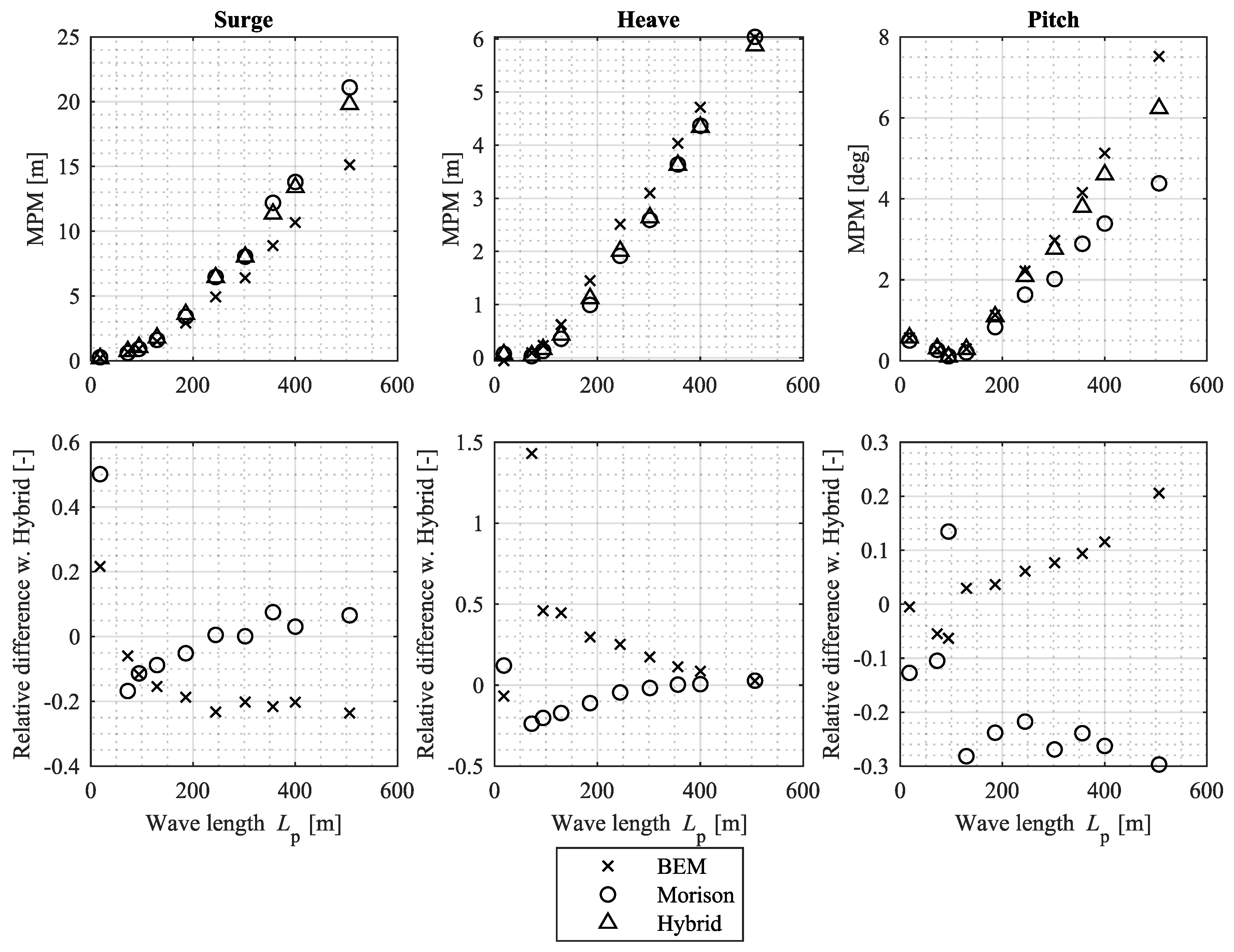
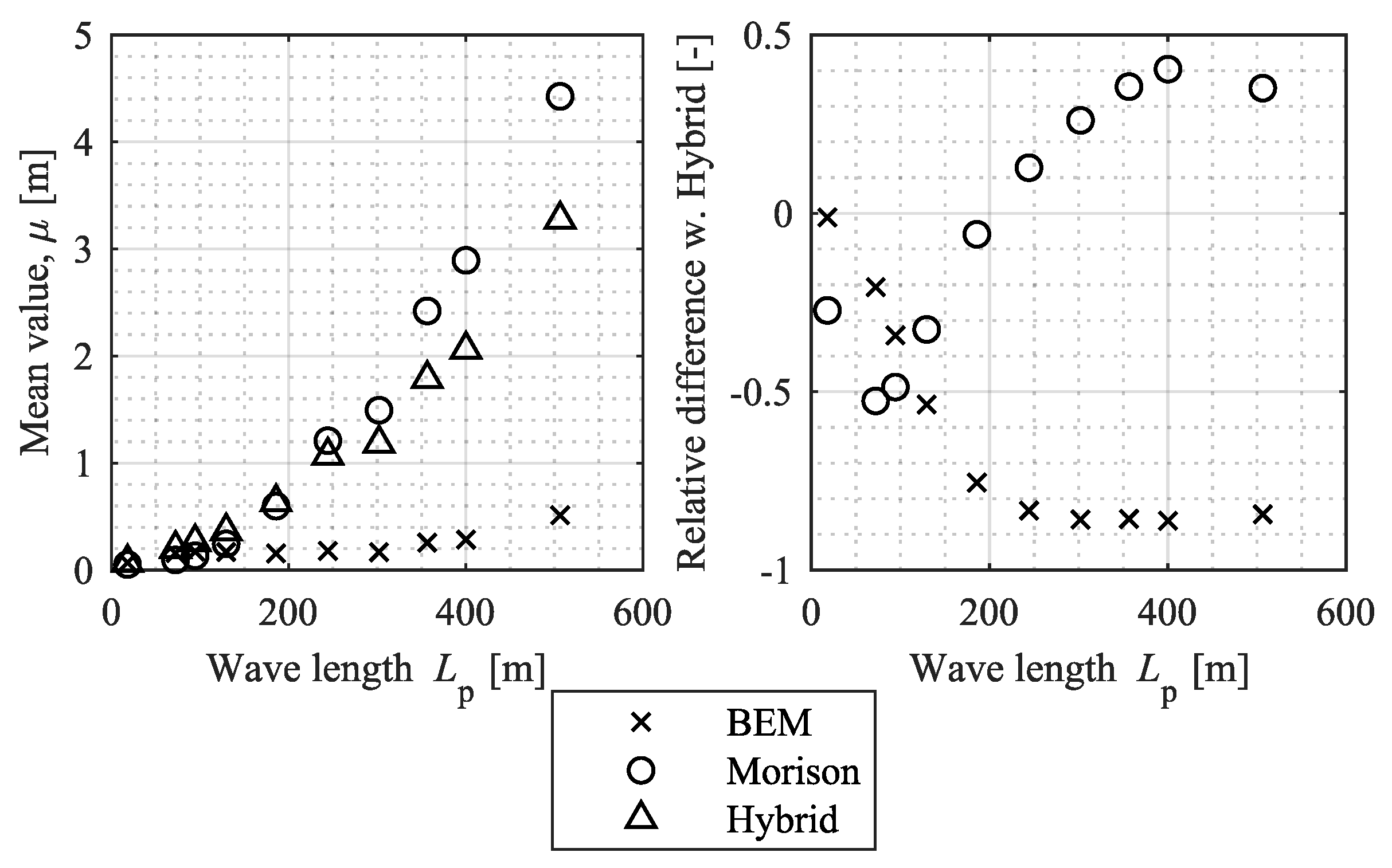
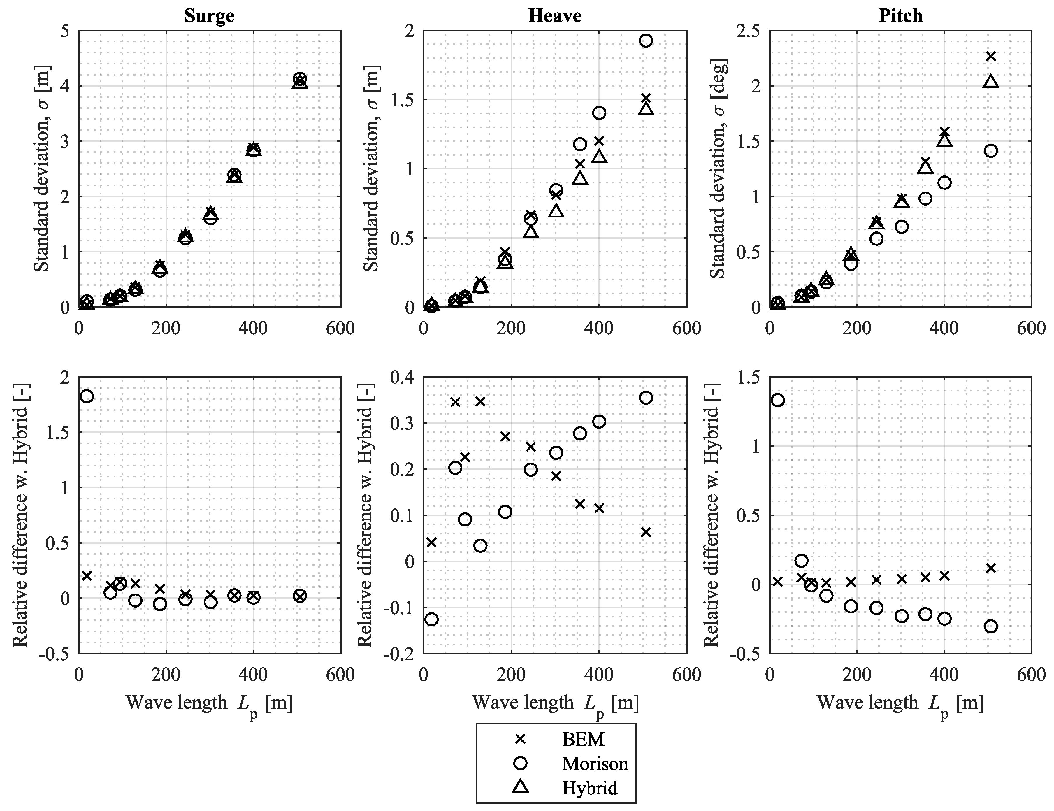
3. Results
4. Discussion and Concluding Remarks
Author Contributions
Funding
Institutional Review Board Statement
Informed Consent Statement
Data Availability Statement
Conflicts of Interest
References
- IRENA. Future of Wind-Deployment, Investment, Technology, Grid Integration and Socio-Economic Aspects; International Renewable Energy Agency (IRENA): Abu Dhabi, United Arab Emirates, 2019. [Google Scholar]
- IRENA. World Energy Transistion Outlook-1.5 °C Pathway; International Renewable Energy Agency (IRENA): Abu Dhabi, United Arab Emirates, 2021. [Google Scholar]
- Wind Europe. Our Energy, Our Future; Wind Europe: Brussels, Belgium, 2019. [Google Scholar]
- BloombergNEF. New Energy Outlook 2020-Executive Summary; BloombergNEF: London, UK, 2020. [Google Scholar]
- Wind Europe. Offshore Wind in Europe–Key Trends and Statistics 2018; Wind Europe: Brussels, Belgium, 2019. [Google Scholar]
- Wind Europe. Floating Offshore Wind; Wind Europe: Brussels, Belgium, 2020. [Google Scholar]
- IRENA. Renewable Power Generation Costs in 2019; International Renewable Energy Agency (IRENA): Abu Dhabi, United Arab Emirates, 2020. [Google Scholar]
- Rsted, O. Making Green Energy Affordable-How the Offshore Wind Energy Industry Matured and What We Can Learn From It; Ørsted: Fredericia, Denmark, 2019. [Google Scholar]
- Wiser, R.; Rand, J.; Seel, J.; Beiter, P.; Baker, E.; Lantz, E.; Gilman, P. Expert elicitation survey predicts 37% to 49% declines in wind energy costs by 2050. Nat. Energy 2021, 6, 555–565. [Google Scholar] [CrossRef]
- Borg, M.; Jensen, M.W.; Urquhart, S.; Andersen, M.T.; Thomsen, J.B.; Stiesdal, H. Technical Definition of the TetraSpar Demonstrator Floating Wind Turbine Foundation. Energies 2020, 13, 4911. [Google Scholar] [CrossRef]
- Stiesdal. The TetraSpar Full-Scale Demonstration Project. 2021. Available online: https://www.stiesdal.com/offshore-technologies/the-tetraspar-full-scale-demonstration-project/ (accessed on 5 May 2021).
- Borg, M.; Viselli, A.; Allen, C.K.; Fowler, M.; Sigshøj, C.; Grech La Rosa, A.; Andersen, M.T.; Stiesdal, H. Physical Model Testing of the TetraSpar Demo Floating Wind Turbine Prototype. In Proceedings of the ASME 2019 2nd International Offshore Wind Technical Conference (IOWTC), Saint Julian’s, Malta, 3–6 November 2019; American Society of Mechanical Engineers Digital Collection: New York, NY, USA, 2019. [Google Scholar]
- Bredmose, H.; Borg, M.; Pegalajar-Jurado, A.; Nielsen, T.R.; Madsen, F.J.; Lomholt, A.K.; Mikkelsen, R.; Mirzaei, M. TetraSpar Floating Wind Turbine Scale Model Testing Summary Report; Technical Report forINNWIND.EU; DTU: Roskilde, Denmark, 2017; Volume 1. [Google Scholar]
- Thomsen, J.B.; Têtu, A.; Andersen, M.T. Experimental Testing of the TetraSpar in Towing and Installation Configuration; Department of the Built Environment: Aalborg, Denmark, 2020. [Google Scholar]
- Pereyra, B.T.; Jiang, Z.; Gao, Z.; Andersen, M.T.; Stiesdal, H. Parametric study of a counter weight suspension system for the tetraspar floating wind turbine. In Proceedings of the International Offshore Wind Technical Conference (IOWTC), San Francisco, CA, USA, 4–8 November 2018; American Society of Mechanical Engineers: New York, NY, USA, 2018; Volume 51975, p. V001T01A003. [Google Scholar]
- Pegalajar-Jurado, A.; Madsen, F.J.; Bredmose, H. Damping Identification of the TetraSpar Floater in Two Configurations With Operational Modal Analysis. In Proceedings of the International Offshore Wind Technical Conference (IOWTC), Saint Julian’s, Malta, 3–6 November 2019; American Society of Mechanical Engineers: New York, NY, USA, 2019; Volume 59353, p. V001T01A024. [Google Scholar]
- Bach-Gansmo, M.T.; Garvik, S.K.; Thomsen, J.B.; Andersen, M.T. Parametric Study of a Taut Compliant Mooring System for a FOWT Compared to a Catenary Mooring. J. Mar. Sci. Eng. 2020, 8, 431. [Google Scholar] [CrossRef]
- Morison, J.R.; Johnson, J.W.; Schaaf, S.A. The force exerted by surface waves on piles. J. Pet. Technol. 1950, 2, 149–154. [Google Scholar] [CrossRef]
- Newman, J.N. Marine Hydrodynamics; MIT Press: Cambridge, MA, USA, 1977. [Google Scholar]
- Faltinsen, O. Sea Loads on Ships and Offshore Structures; Cambridge University Press: Cambridge, MA, USA, 1993; Volume 1. [Google Scholar]
- Falnes, J. Ocean Waves and Oscillating Systems: Linear Interactions Including Wave-Energy Extraction; Cambridge University Press: Cambridge, MA, USA, 2002. [Google Scholar]
- Lee, C.H.; Newman, J.N. WAMIT User Manual; WAMIT, Inc.: Chestnut Hill, MA, USA, 2006. [Google Scholar]
- DNV-GL. Position Mooring; DNV-GL Offshore Standard DNVGL-OS-E301; DNV-GL: Høvik, Norway, 2018. [Google Scholar]
- DNV-GL. Environmental Conditions and Environmental Loads; DNV-GL Recommended Practice DNVGL-RP-C205; DNV-GL: Høvik, Norway, 2010. [Google Scholar]
- IEC. Wind Energy Generation Systems-Part 3-2: Design Requirements for Floating Offshore Wind Turbines; International Electrotechnical Commission (IEC): Geneva, Switzerland, 2019. [Google Scholar]
- DNV-GL. Floating Wind Turbine Structures; DNV-GL Offshore Standard DNVGL-ST-0119; DNV-GL: Høvik, Norway, 2018. [Google Scholar]
- Thomsen, J.B.; Ferri, F.; Kofoed, J. Validation of a Tool for the Initial Dynamic Design of Mooring Systems for Large Floating Wave Energy Converters. J. Mar. Sci. Eng. 2017, 5, 45. [Google Scholar] [CrossRef] [Green Version]
- Orcina Ltd. Orcina. 2021. Available online: https://https://www.orcina.com/ (accessed on 5 May 2021).
- Orcina Ltd. OrcaFlex User Manual; Orcina Ltd.: Ulverston, UK, 2021. [Google Scholar]
- Babarit, A.; Delhommeau, G. Theoretical and numerical aspects of the open source BEM solver NEMOH. In Proceedings of the 11th European Wave and Tidal Energy Conference (EWTEC2015), Nantes, France, 6–11 September 2015. [Google Scholar]
- Orcina Ltd. OrcaWave User Manual; Orcina Ltd.: Ulverston, UK, 2021. [Google Scholar]
- Cummins, W. The Impulse Response Function and Ship Motions; Technical Report; David Taylor Model Basin: Washington, DC, USA, 1962. [Google Scholar]
- Newman, J. Second-Order, Slowly-Varying Forces on Vessels in Irregular Waves; Massachusetts Institute of Technology, MIT Press: Cambridge, MA, USA, 1974. [Google Scholar]
- Chakrabarti, S. Handbook of Offshore Engineering; Elsevier: Amsterdam, The Netherlands, 2005. [Google Scholar]
- Newman, J.N. Wave-drift damping of floating bodies. J. Fluid Mech. 1993, 249, 241–259. [Google Scholar] [CrossRef]


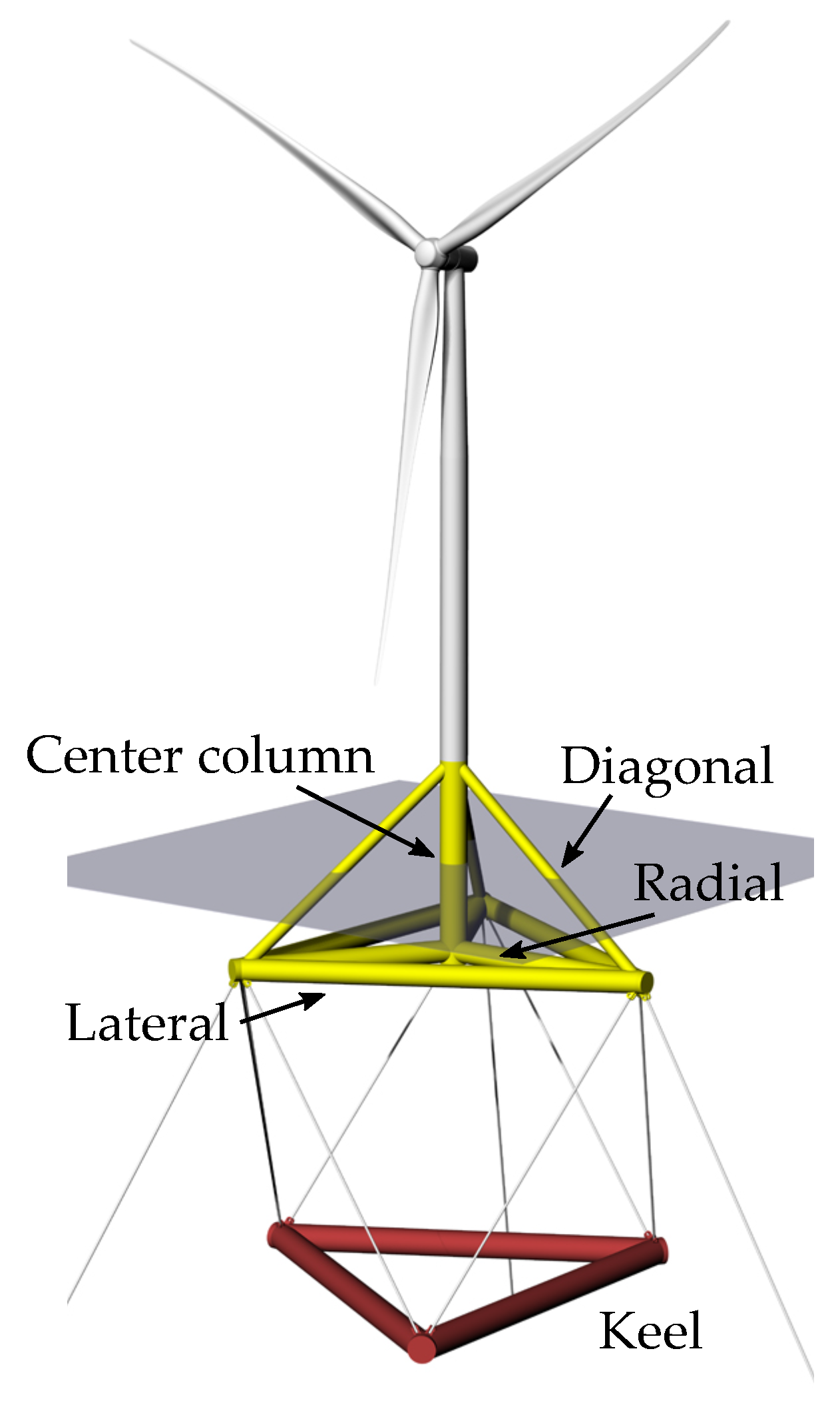
| Element | Diameter (m) |
|---|---|
| Center column | 4.3 |
| Lateral | 4.1 |
| Radial | 3.5 |
| Diagonal | 2.0 |
| Keel | 4.3 |
| Case | Significant Wave Height, (m) | Peak Wave Period, (s) | Peak Wave Length, (m) | Water Depth, (m) |
|---|---|---|---|---|
| Operational, O1 | 0.4 | 3.40 | 18.1 | 220.0 |
| Operational, O2 | 1.8 | 6.8 | 72.3 | 220.0 |
| Operational, O3 | 2.5 | 7.8 | 94.4 | 220.0 |
| Operational, O4 | 3.6 | 9.1 | 129.4 | 220.0 |
| Operational, O5 | 5.7 | 10.9 | 185.7 | 220.0 |
| Operational, O6 | 8.0 | 12.5 | 244.2 | 220.0 |
| Extreme, E1 | 9.3 | 13.9 | 302.0 | 220.0 |
| Extreme, E2 | 11.4 | 15.1 | 356.4 | 220.0 |
| Extreme, E3 | 12.9 | 16.0 | 400.1 | 220.0 |
| Extreme, E4 | 16.3 | 18.0 | 506.4 | 220.0 |
| Coefficient | Value |
|---|---|
| 1.05 | |
| 1.0 | |
| 2.0 |
| Morison Approach | BEM Approach | Hybrid Approach | ||||
|---|---|---|---|---|---|---|
| Inertia | ||||||
| Froude–Krylov | ✔ | Instantaneous | ✔ | Freq. dependent | ✔ | Freq. dependent |
| submerged volume | ||||||
| Added mass | ✔ | Constant | ✔ | Freq. dependent | ✔ | Freq. dependent |
| Diffraction | ✘ | ✔ | Freq. dependent | ✔ | Freq. dependent | |
| Radiation | ✘ | ✔ | Freq. dependent | ✔ | Freq. dependent | |
| Drag | ✔ | Constant | ✘ | ✔ | Constant | |
| Scaled to wet area | Scaled to wet area | |||||
| Damping | ||||||
| Linear | ✔ | Constant, | ✔ | Freq. dependent | ✔ | Freq. dependent |
| radiation damping | radiation damping | |||||
| Quadratic | ✔ | Viscous damping | ✘ | ✔ | Viscous damping | |
| from | from | |||||
| Wave drift | ✔ | From motion | ✔ | From QTF | ✔ | From QTF and |
| damping | response | motion response | ||||
| Wave Drift | ✔ | From and with | ✔ | From QTF | ✔ | From QTF and , |
| instantaneous area | instantaneous area | |||||
| and displaced volume | and non-linear | |||||
| Non-linear waves | waves | |||||
| Stiffness | ✔ | Non-linear hydro- | ✔ | Non-linear hydro- | ✔ | Non-linear hydro- |
| static stiffness | static stiffness | static stiffness | ||||
| Component | O1 | O2 | O3 | O4 | O5 | O6 | E1 | E2 | E3 | E4 |
|---|---|---|---|---|---|---|---|---|---|---|
| Center column | 0.42 | 0.60 | 0.63 | 0.65 | 0.67 | 0.67 | 0.67 | 0.67 | 0.67 | 0.67 |
| Lateral | 0.40 | 0.60 | 0.62 | 0.65 | 0.67 | 0.67 | 0.67 | 0.67 | 0.67 | 0.67 |
| Radial | 0.30 | 0.50 | 0.55 | 0.60 | 0.65 | 0.65 | 0.67 | 0.67 | 0.67 | 0.67 |
| Diagonal | 0.30 | 0.45 | 0.50 | 0.55 | 0.60 | 0.62 | 0.62 | 0.65 | 0.65 | 0.65 |
| Original value (all elements) | 1.05 | |||||||||
| Morison | |||||||
|---|---|---|---|---|---|---|---|
| Original | Updated | BEM | Hybrid | ||||
| Parameter | Value | Rel. diff. | Value | Rel. diff. | Value | Rel. diff. | Value |
| (m) | 0.052 | 0.72 | 0.052 | 0.72 | 0.071 | 0.99 | 0.072 |
| (m) | 0.103 | 2.86 | 0.070 | 1.94 | 0.044 | 1.22 | 0.036 |
| (m) | 0.404 | 2.02 | 0.294 | 1.47 | 0.222 | 1.11 | 0.200 |
Publisher’s Note: MDPI stays neutral with regard to jurisdictional claims in published maps and institutional affiliations. |
© 2021 by the authors. Licensee MDPI, Basel, Switzerland. This article is an open access article distributed under the terms and conditions of the Creative Commons Attribution (CC BY) license (https://creativecommons.org/licenses/by/4.0/).
Share and Cite
Thomsen, J.B.; Têtu, A.; Stiesdal, H. A Comparative Investigation of Prevalent Hydrodynamic Modelling Approaches for Floating Offshore Wind Turbine Foundations: A TetraSpar Case Study. J. Mar. Sci. Eng. 2021, 9, 683. https://doi.org/10.3390/jmse9070683
Thomsen JB, Têtu A, Stiesdal H. A Comparative Investigation of Prevalent Hydrodynamic Modelling Approaches for Floating Offshore Wind Turbine Foundations: A TetraSpar Case Study. Journal of Marine Science and Engineering. 2021; 9(7):683. https://doi.org/10.3390/jmse9070683
Chicago/Turabian StyleThomsen, Jonas Bjerg, Amélie Têtu, and Henrik Stiesdal. 2021. "A Comparative Investigation of Prevalent Hydrodynamic Modelling Approaches for Floating Offshore Wind Turbine Foundations: A TetraSpar Case Study" Journal of Marine Science and Engineering 9, no. 7: 683. https://doi.org/10.3390/jmse9070683
APA StyleThomsen, J. B., Têtu, A., & Stiesdal, H. (2021). A Comparative Investigation of Prevalent Hydrodynamic Modelling Approaches for Floating Offshore Wind Turbine Foundations: A TetraSpar Case Study. Journal of Marine Science and Engineering, 9(7), 683. https://doi.org/10.3390/jmse9070683