Abstract
Extensive electrification of ship power systems appears to be a promising measure to meet stringent environmental requirements. The concept is to enable ship power management to allocate loads in response to load variations in an optimal manner. From a broader design perspective, the reliability of machinery operation is also of importance, especially with regard to the failure cost from power outages. In this paper, an approach for determining optimal power plants based on economic and environmental perspectives across several architecture choices is proposed. The design procedure involves the implementation of metaheuristic optimization to minimize fuel consumption and emissions released, while maintenance and repair services can be extracted using reliability assessment tools. The simulation results demonstrated that ship power management using the whale optimization algorithm (WOA) was able to reduce fuel consumption and corresponding emissions in a range from 4.04–8.86%, varying with the profiles, by eliminating inefficient working generators and distributing loads for the rest to the nearest possible energy-saving areas. There was also a trade-off between maintenance service and overall system expenses. Finally, a compromise solution was sought with the proposed holistic design for contradictory cost components by taking into account fuel operation consumption, shore electricity supply, maintenance service and investment expenditure.
1. Introduction
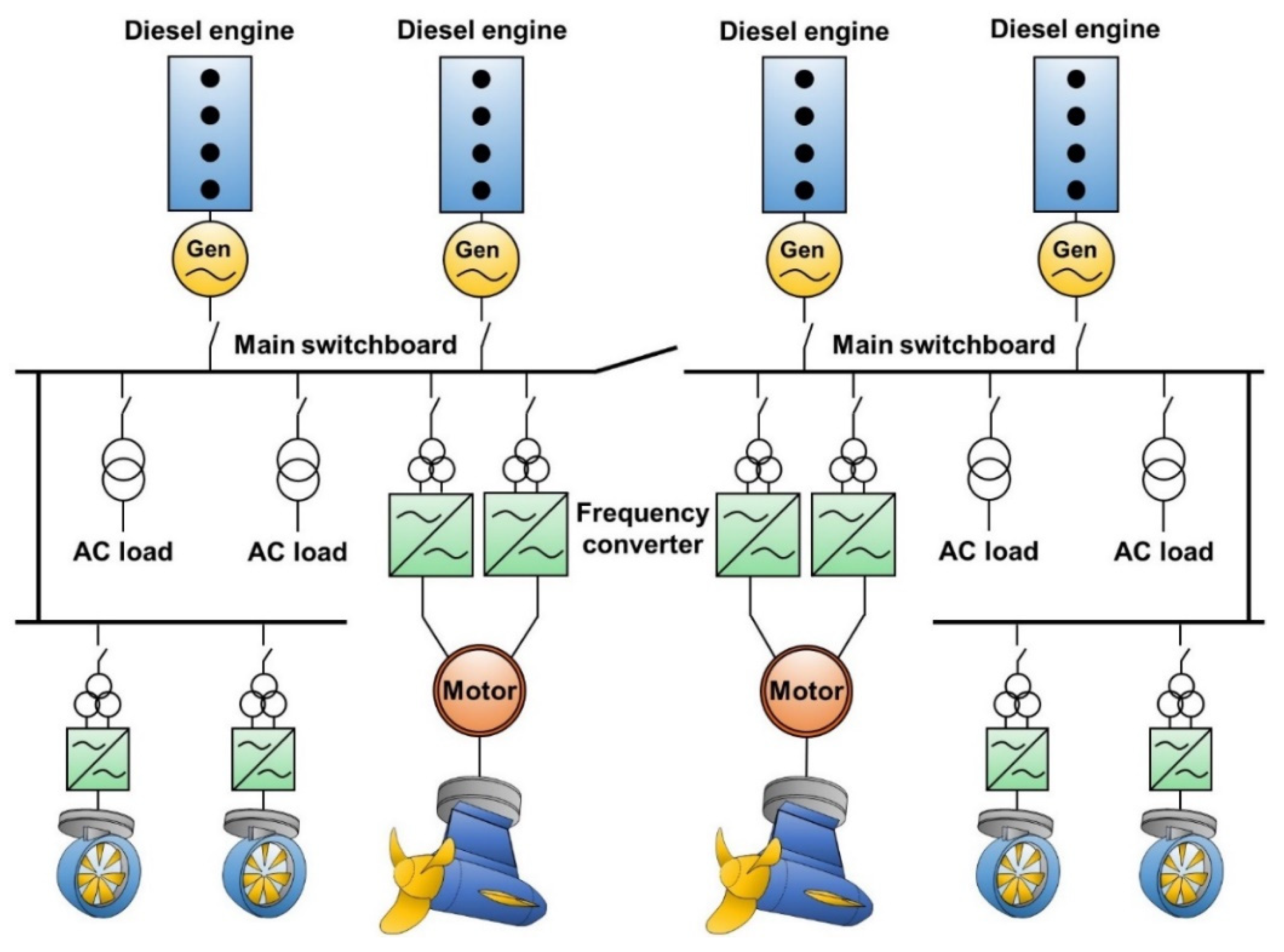
Cruise tourism in recent decades has experienced impressive growth in terms of itineraries and passenger sourcing. However, the total greenhouse gas (GHG) emissions of global marine transport have also increased to 1076 million tons in 2018, which corresponds to a 2.89% share in global anthropogenic pollution [1]. Consequently, there is mounting concern over the environmental impact due to maritime traffic emissions. Various measures including fuel-efficient technologies and environmental policies are therefore being proposed to make onboard energy systems more efficient [2,3]. Extensive electrification through integrated electric propulsion platforms appears to be a cost-effective and emission-aware solution to conform to the tightening restrictions of energy efficiency directives [4]. As shown in Figure 1, a typical system platform for diesel-electric cruise passenger ships is comprised of diesel generator sets connected with main switchboard panels. The electrical power is then distributed to accommodate all electrical loads throughout the ship, including propulsion motors via variable frequency drives. This centralized power concept enables various optimization techniques through ship power management to optimally allocate loads for individual power generation sources [5]. A fuel cost reduction hence can be achieved by economic load distribution and minimization of active generator sets. By implementing holistic cost-effective design, the reliability of machine operation should also be taken into consideration, particularly with regard to the consequences of failure incidents. Over the past decade, machinery breakdown, including engine failure, has risen as one of the largest causes of marine insurance claims [6]. Such a failure trend is unlikely to change anytime soon and has been anticipated to increase in severity, driven by the escalating cost of repair services and as a consequence of larger vessels. In this study, a design scheme taking into account ship power management and reliability attributes was devised to determine the optimal power plants to be installed such that the system is able to be maintained in spite of load variations with the lowest fuel consumption and failure costs.
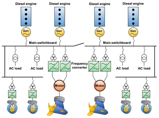
Figure 1.
Typical integrated electric propulsion for cruise ships.
Research on ship power management usually contends with energy flows and power distribution challenges. Load allocation optimization by dynamic programming (DP)-based algorithms was proposed for an electric ferry in [7] and hybrid propulsion in [8]. Optimized power management or such management in combination with ship speed adjustments can save fuel operation costs by 2.86% and 3.80% respectively. A combination of sequential quadratic programming (SQP) and branch-and-bound methods was proposed in [9] in order to optimally allocate independent demands of mechanical, electrical and thermal energy. The results demonstrate the possibility that annual fuel saving of up to 3% can be achieved. The use of the genetic algorithm (GA) with the introduction of additional thermal components is described in [10]. The study demonstrated that thermal storage and absorption chillers can account for emission reductions of up to 20%. The success of applying the GA was also demonstrated in [11], in which a triple optimization problem (synthesis–design–operation) could be solved by a single-level procedure in order to minimize the risk of excluding the global optimum. A fuzzy-based particle swarm optimization (PSO) technique was applied to a shipboard energy storage system in [12]. The proposed technique ensured the produced CO2 per unit of transport work was well below a threshold and could reduce fuel costs by 6.36%. The PSO algorithm was combined with the non-dominated sorting genetic algorithm II (NSGA-II) to solve a multi-objective problem in [13]. By further considering voyage optimization and integration of thermal storage, the fuel costs and GHG emissions could be reduced by 17.4% and 23.6%, respectively.
The optimization results from the above survey seem to reveal the limitations of pure optimization in dealing with non-smooth and non-convex cost functions in marine electrical dispatch due to the nonlinear characteristics of various technical constraints. The classical methods are likely to suffer from the computation of first- or second-order derivatives and high sensitivity to initial searching areas eventually leading to local optima convergence or their divergence altogether [14]. Metaheuristic techniques can therefore be introduced to eradicate such difficulties thanks to their derivative-free mechanisms and stochastic nature which allows them to bypass local optima and explore the entire search space extensively.
With regard to ship configuration design, most published studies only give special attention to environmental and economic pressures. An overview of technological research in ship power system design is provided in [15]. The increasing use of sophisticated power electronics onboard is leading to innovative designs through the implementation of key performance indicators (KPIs) such as efficiency, reliability and safety. This in turn also means a move towards reducing both capital investment and operational expenditure. A system design process aimed at analyzing dependability attributes is presented in [16]. A fault forecasting technique is used to identify critical failure points such that corrective solutions can be applied beforehand. The evaluation of the system response to faults and the effectiveness of the solutions can then be processed through modeling and iterative simulation. The use of classifier-guided sampling (CGS) to identify survivable configurations for zonal ship design is described in [17]. The methodology involves analyzing and placing heat dissipation and electrical distribution components into optimal locations for damages scenarios. The selection of prime movers and energy storage options also plays a crucial role in enhancing survivability characteristics and other objectives, like operation cost, mission capability and reliability. A framework for determining optimal propulsion plants based on life cycle cost (LCC) is given in [18]. The structure of the design process is comprised of construction, operation, maintenance and scrapping stages. The results demonstrate that hybrid ship configurations consisting of several sets of engines are the most desirable. The optimal design of hybrid electric propulsion is presented in [19] by investigating the trade-off between fuel consumption, GHG emissions and life cycle cost. A multi-objective optimization method applied to a hybrid diesel/battery/shore power system is able to significantly reduce all three objectives as compared to single objective optimization and conventional propulsive systems. The multi-objective optimization can also be used to appropriately size system components, such as diesel engine displacement, motor rotor diameter and the number of battery modules, as proposed in [20]. Optimal configurations that result from a combination of various alternative technologies have been proposed for the requirements of environmental and economic sustainability in [21] and under the impact of carbon pricing scenarios in [22]. The application of dual fuel engines operating with natural gas is considered a cost-effective solution, while the combination of fuel cells and carbon capture technology is identified as leading to the greatest reduction of emissions released. The optimization of ship power plants in light of economic, environmental and safety criteria in a life cycle basis are investigated in [23]. The potential best alternative option involves the installation of dual fuel generator sets to improve economic and environmental performance without increasing the risk of system blackout. Various machinery system arrangements in combination with emission control plans were compared and analyzed in terms of flexibility and robustness in [24]. The robust solution should be able to withstand future emission controls without retrofitting the system, whereas the flexible configuration allows the implementation of necessary measures in the face of stringent environmental regulations.
The literature survey indicates that a research opportunity exists to identify optimal ship power plants by way of bringing down all operating cost components. The conventional design of power plants usually involves the selection of prime movers and configuration arrangements that should satisfy power demands at all operating points. Alternative system designs such as hybrid propulsion may be additionally taken into consideration as introduced in available published work. However, such a design procedure virtually excludes the energy-saving function of ship power management that, to a significant extent, affects the total amount of fuel consumption, particularly in the ship operation design phase. In other words, the operating conditions of individual prime movers are disregarded or treated as unoptimized conditions over the entire operation period. Moreover, the maintenance and repair services which contribute substantially to the whole-life operating costs are often neglected or estimated without considering the consequence of occurred failures. In practice, the reliability objective should be given top priority and taken into consideration at the early stage of system design to ensure safety operation and minimum failure costs.
The methodology proposed here is equipped to handle such challenges by incorporating ship power management and reliability features into the design. In more detail, the proposed power management is able to optimally allocate loads for minimizing fuel operation costs via recently developed metaheuristic optimization methods which in general demonstrate greater achievements in terms of cost-effective solutions, accuracy and convergence. The optimization performance is measured for different load profiles and by comparing various optimization techniques. The procedure also accommodates the need to be environmentally friendly through the introduction of real-world emission regulations. The maintainability perspective is then assessed, in the form of maintenance and repair service expenditure, by reliability tools. Finally, the decision-making process for the installation of system plants across several architecture choices is considered in relation to ship lifetime operating costs, taking into account variations of fuel and non-fuel operation expenses, and by consideration of changes in the present value over time. Although the case study chosen in this work concerns diesel-electric ship propulsion, the developed design scheme can also be applied for terrestrial power plants and alternative marine power systems.
The main novelties and contributions of this study can be summarized as follows:
- A design procedure is devised for determining optimal ship power plants that are able to minimize lifetime operating costs through consideration of the minimization of fuel operation, shore electricity supply, maintenance service and investment expenditure;
- Optimization of ship power management can be implemented by means of asymmetric load sharing and metaheuristic techniques. The load allocation problem is formulated under technical constraints and real-world emission regulations;
- Power plant configurations can be designed in accordance with emission control, reliability and economic requirements. The design scheme described here has the potential to be established in any electric propulsion platform through modifications of the power generation components.
This article is organized as follows: Section 2 provides an overview of the system configuration design procedure. Section 3 provides details on assessment criteria. Section 4 goes through the process of solving a formulated optimization problem. Simulation results based on actual ship voyages and various configuration designs are discussed in Section 5 and finally conclusions are given in Section 6.
2. Cruise Ship Power Plant Configuration Design
A ship power system can to some extent be considered a terrestrial microgrid due to its clearly defined electrical boundary and independent operation capability [25]. It can be characterized as an isolated and self-sufficient system during its time in the open sea and it becomes part of the terrestrial grid when connecting to shore-side power supply. However, ships have a greater incentive for reliability design because of the required safety of passengers and the considerable cost associated with power failures. Due to this isolated nature, a high level of security and redundancy is absolutely crucial and must be considered at the early design stage. According to related ship classification rules, there must be continuity of sufficient electrical power to supply essential services such that the ship is able to retain not less than 50% of the prime mover capacity in the event of one power generation failure [26]. The reliable ship power plant thus has to be designed according to the load demand under the most likely scenarios. The rating and quantity of prime movers can also be defined by the requirement of maximizing energy efficiency and by a loading capability that can satisfy the highest anticipated demand.
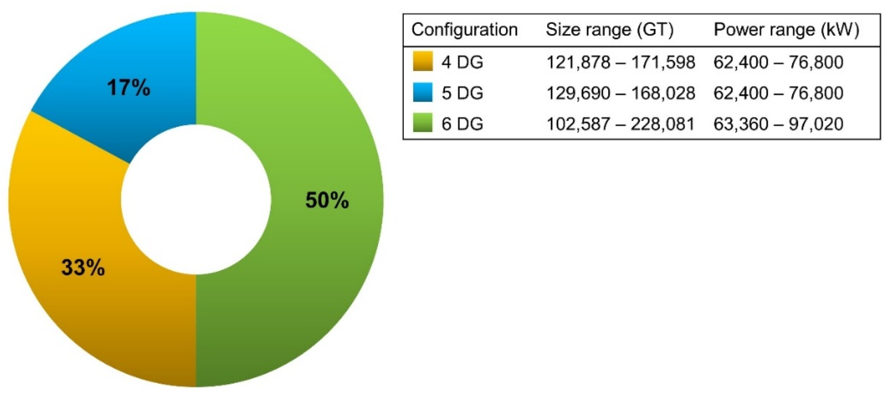
Based on a survey of large diesel-electric cruise ships with gross tonnage greater than 100,000 GT, power plant design predominantly consists of three configurations, namely four, five and six diesel generator (DG) systems, as shown in Figure 2. The survey data indicate that ship sizes from 102,587 GT to 228,081 GT have installed power capacities varying from 62,400 kW to 97,020 kW. The 6-DG configuration constitutes the majority of power plant designs, followed respectively by the 4-DG and 5-DG systems. There is no distinct difference between 4-DG and 5-DG arrangements in terms of gross tonnage and installed power. However, when the size of ships is increased to that of the largest vessels, the 6-DG architecture is reserved as the design to be installed.

Figure 2.
Conventional power plant configurations for large diesel-electric cruise ships.
The procedure for determining optimal power plant design begins with the determination of operation load profiles and information on the planned itinerary of a cruise ship on order. System configuration can be designed on the basis of technical constraints, such as installation power and the number of generation plants. Power management through load allocation optimization can be established to meet the requirements of minimizing the fuel consumption and the GHG emissions released. The algorithm selection process is based on the optimization performances measured for certain load profiles, comparing them with various optimization techniques. For ships operating at berth, the port operation costs can be estimated by applying a cold ironing concept. The maintainability of architecture can be determined by reliability assessment tools in order to extract the corresponding maintenance and repair service costs. Finally, the lifetime operation expense is estimated through the trajectories of fuel oil, shore electricity and upkeep service expenditures, considering monetary value over time. For system designs with variations in the installed power, the overall system cost can be taken into account. Other contributing factors, such as system weight and volume, as well as downtime costs associated with propulsion failures, may also be included, but they will not be further investigated in this work.
The study assumed the procedure was applied to a new vessel on order in the same class as the MV Britannia, a diesel-electric cruise ship operating in the European seas. The ship is equipped with twin 18,000 kW electric propulsion motors and four medium-speed diesel engines producing total power of 62,400 kW. As a basis for comparison, three conventional potential designs, restricted by the original engine brake power, are described. One configuration consists of four prime movers, as previously installed. The other two configurations deploy five and six prime movers. Accordingly, the engine rating selection for the latter two arrangements is modified according to the required number of prime movers and the restriction in the total installed power. Table A1 summarizes the parameters and configuration designs for the Britannia-class vessel.
3. Assessment Criteria
3.1. Environmental Assessment
3.1.1. Ship Energy Efficiency
The standard indicator to evaluate the performance of energy systems for ships in service is the energy efficiency operational indicator (EEOI). As defined by the International Maritime Organization (IMO), ship energy efficiency correlates with the amount of fuel consumed with respect to the transport work carried out [27]:
where EEOI is expressed as tons CO2/GT nautical mile; f is the fuel type; FC is the mass of consumed fuel (tons); CF is the fuel mass to CO2 mass conversion factor (ton CO2/ton fuel); GT is the ship gross tonnage; V is the ship speed (knots); and Δt is the time interval.
3.1.2. Combustion Emissions
According to the IMO methodology, the current practice to estimate gaseous emissions resulting from engine combustion is based on multiplication of emission factors and fuel consumed [28]. The values of emission factors can vary according to engine type, fuel type, fuel sulfur content and the emission standards used:
where e is the substance of emission; f is the fuel type; g is the engine type; P is the instantaneous engine power (kW); SFC is the specific fuel consumption (g/kWh); and EF is the emission factor of the substance (ton/ton fuel).
3.2. Reliability Assessment
To date, there have been no methods developed in the maritime industry to quantify the reliability improvement resulting from the adjustment of propulsion redundancy. The practice for the design of reliable industrial and commercial power systems [29] is therefore adopted by considering the ship power system as a terrestrial microgrid [30].
The term “engineering reliability” refers to the probability of a system performing required functions under stated condition in a certain time. The reliability evaluation is typically described by the exponential failure distribution characterized by a constant failure rate . The failure density function for the time to failure t is given by
The cumulative failure function represents the unreliability or cumulative probability of a failure occurring before a certain time.
The reliability function represents the probability that a failure has not occurred by given time.
The inverse of the failure rate is the mean time to failure (MTTF), which describes the expected time that a system functions properly before a failure occurs.
For a repairable system, the mean time between failures (MTBF) is recommended to be used in conjunction with the mean time to repair (MTTR), which refers to the mean downtime between consecutive failures.
For system architecture with a series configuration, the total reliability is taken to be a product of the component reliability. Hence, the system reliability cannot be greater than the least reliable component. Accordingly, a significant improvement over the series configuration can be secured with a redundancy design concept. By defining N as the required number of components to successfully operate the system, the N + X topology ensures enough capacity in case of the failure of X components. This type of redundant structure can also be described as a system that requires at least k-out-of-n parallel elements to function, as follows:
The system MTTF and MTTR can be extracted by:
where k indicates the required generators to be operated, n is the total number of installed generators and is a constant repair rate.
With respect to more complicated reliability designs, a special case of parallel redundancy named weighted k-out-of-n can be considered. This terminology is a variation of the binary k-out-of-n system that includes contributions or weights of components in the calculation [31]. In the present case, by assuming that the component reliability is identical for all generation sets and by classifying the n generators into weight classes with respect to generation capacity, i.e. weight w1 for nH high-rating generators and w2 for nL low-rating generators, the system is supposed to successfully function only if the total weight of all working generators is no less than the load demand k. The reliability for such a case can be computed by the following recursive equations:
The extraction of the system MTTF requires a particular equation [32]:
where B(a, b) denotes the beta function and θ = λ2/λ1.
3.3. Economic Assessment
The major contribution to the total variable expense of a ship in service is made by the fuel operation costs. The total fuel expenditure can be simply estimated by the multiplication of fuel consumed during the defined period and the average fuel oil price. For ships operating at berth, it can be assumed that shutting down all generator engines continues as standard practice to eliminate gaseous port pollution and facilitate maintenance of machinery. Thus, the port operation costs can be estimated by the multiplication of the ship average load demand at berth and the shore electricity price. In terms of maintainability, the total maintenance service is comprised of scheduled and unscheduled maintenance.
Scheduled maintenance refers to interval inspections, periodic replacement of materials and scheduled overhauls. The onboard maintenance is generally carried out under service contracts and can be classified into variable and fixed operation and maintenance (O&M) costs. The variable costs refer to a variation of the maintenance expense according to the component operating hours, while the fixed costs are based on a routine basis regardless of the component runtime.
Unscheduled maintenance is represented by repair costs that are directly affected by the system reliability. The costs typically include additional expenditures incurred by random system failures, like replacement of spare parts plus labor charges.
The consolidated maintenance service costs can then be given by:
The lifetime operation costs for the weighted k-out-of-n system, considering the present overtime value, can be eventually estimated by:
where r is a discount rate and L is a project lifetime.
4. Optimization of Power Generation Dispatch
4.1. Modeling of Specific Fuel Consumption
The specific fuel consumption (SFC) of an engine is a measure of the amount of fuel consumed to produce a unit of work and hence in turn measures fuel efficiency. Typically, the SFC model can be to some extent approximated by polynomial or exponential functions. However, in the present study we found spline interpolation to be far preferable, as it is constructed in such a way as to minimize the norm of residues and to reduce oscillation between data points.
The marine engine selected was the Wärtsilä 46F, which is installed for the prime movers on the Britannia. The SFC data for V- and L-type engines at a specific load condition can be obtained from the engine manufacturer [33]. The model then can be represented by extrapolation and cubic spline interpolation functions as follows:
where pj is the power assigned to jth engine.
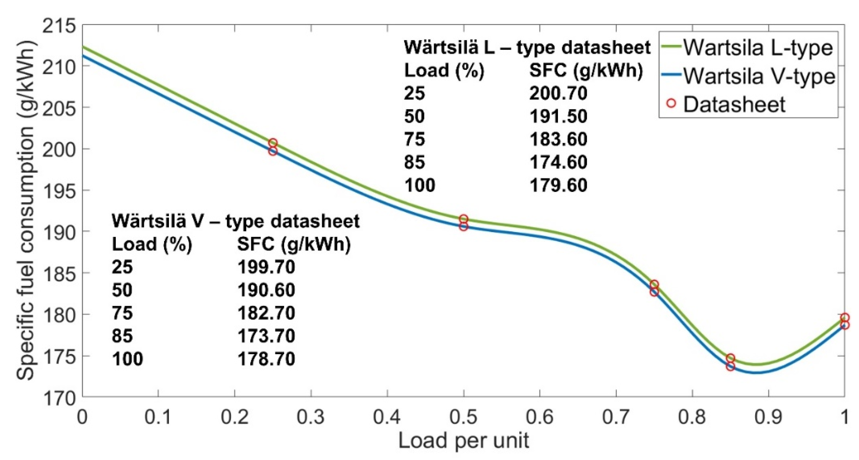
The SFC map derived from the equations is shown in Figure 3. The optimal operating condition for all engine types can be seen to be between 80–90% of the maximum continuous rating (MCR), whereas the lightly loaded engine consumes significantly higher fuel. It is also evident the L-type engine delivers lower fuel efficiency at all operating conditions compared to the V-type engine.
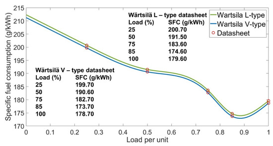
Figure 3.
SFC map of Wärtsilä 46F V- and L-type engines at various loads.
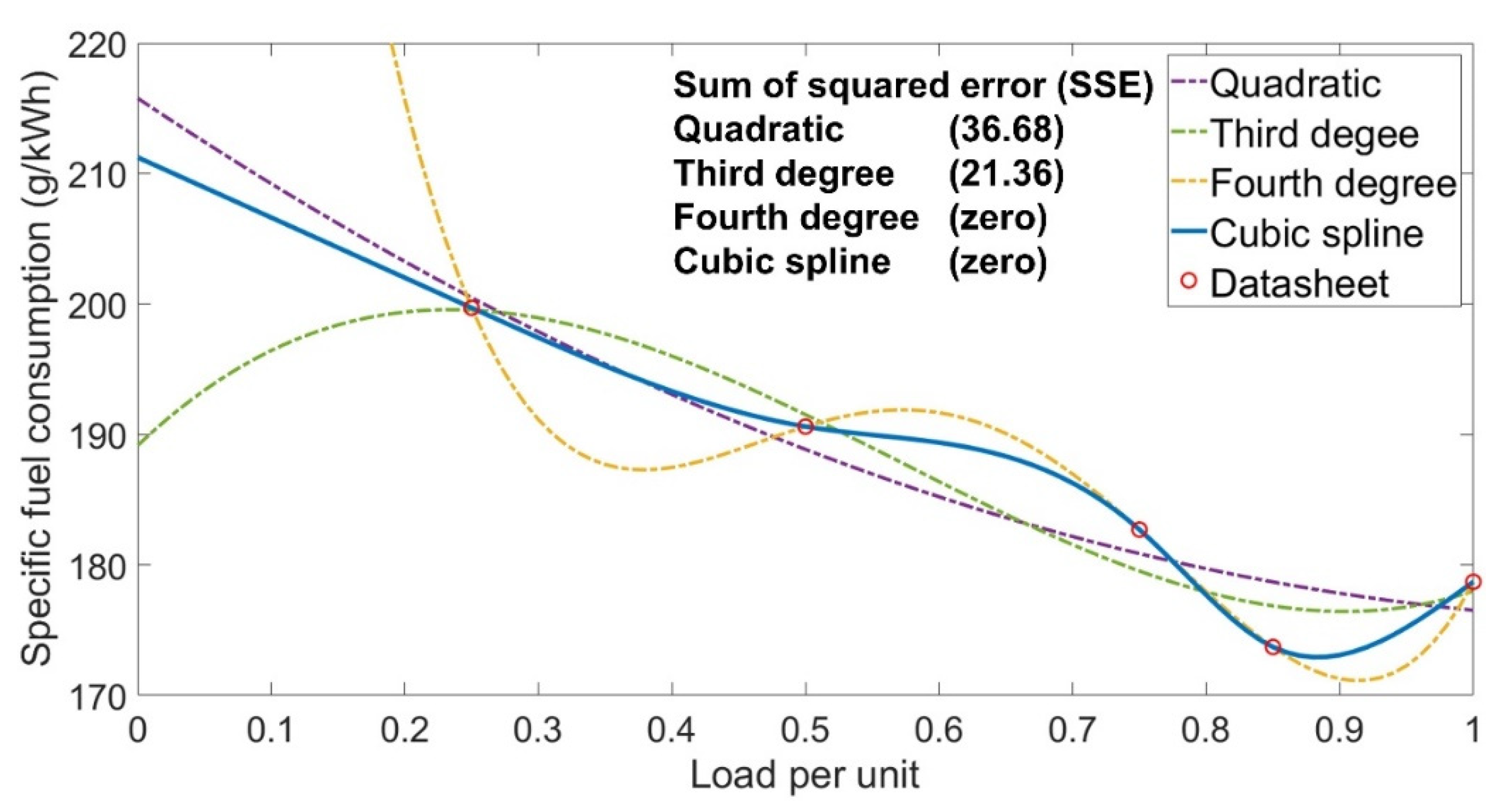
Figure 4 shows a comparison between cubic spline and polynomial interpolation methods. The sum of squared estimate of errors (SSE) can be used to measure the total deviations of the response values from actual empirical data. The accuracy of the polynomial interpolation is commensurate with higher order polynomials and can be comparable with spline interpolation in which zero discrepancy is obtained. However, high degree polynomials severely suffer from Runge’s phenomenon, which refers to a problem of oscillation at the edges of intervals.
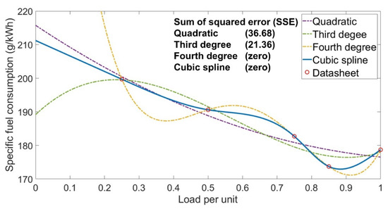
Figure 4.
Comparison of interpolation methods.
4.2. Optimization Problem Formulation
The objective of the power generation dispatch is to minimize total fuel consumption governed by constraints. The ship power management should be able to automatically activate and deactivate each individual generator in order to coincide with instantaneous load variations and also to keep the average engine loading as close as possible to an efficient area through an asymmetric load sharing principle. The optimization problem can be formulated as follows.
By considering N engine generators and by assuming that the rated power of the Nth engine is maximum, the rating of each prime mover to the base of the maximum is given per unit (pu) by:
The power assigned to the jth engine at time interval Δti is given by pj,i and its specific fuel consumption is defined as SFC(pj,i). The total fuel consumed by all engines for the time horizon Thorizon is given by:
The optimization problem can then be formulated as:
The constraints of the optimization problem can be defined as follows:
(1) The generation power must be equal to the total load demand:
where Ptotal,Δti is the total power demand at time interval Δti.
(2) The generated power is constrained by the generation capability of a generator:
where .
(3) An increase in the speed and load of a start-up engine is restricted by the allowed load increase rate:
where Rstart-up is the maximum allowed load increase rate for a start-up engine.
(4) The speed and load ramp-up/down of an engine is restricted by the load acceptance capability:
where Rup/down is the maximum permissible instant load step.
(5) Optimization attempting to minimize total fuel consumption should also aim at reducing GHG emissions or the EEOI over the entire operation:
4.3. Implementation of Metaheuristic Optimization
This section provides brief details on a metaheuristic inspired by the social synergy of humpback whales, namely the whale optimization algorithm (WOA), for use in solving the formulated problem. The algorithm was originally developed by Mirjalili and Lewis [34] and has been increasingly tailored in a wide range of engineering applications, especially research work related to economic load dispatching [35]. The algorithm was also selected as it employs swarm-based solutions, which represent a number of candidates moving around the search space. In other words, the swarm (all candidates) traces the best location in its path and meanwhile each individual also traces its own best position. This technique has been proven to be very competitive on the basis of its capacity to memorize explored path information over the course of iterations, while evolution-based solutions, like the GA, eliminate all explored space over subsequent generations. Also, swarm intelligence is usually implemented with fewer operators and hence it is simpler to code.
The WOA mimics a special hunting method of swarms of humpback whales called the bubble-net hunting strategy. The whales generate bubbles in a spiral shape to surround prey, keeping them from escaping. All whales then simultaneously swim up toward the surface to feed on the trapped prey. This strategic maneuver can be mathematically modeled on the basis of foraging mechanisms, namely exploitation and exploration.
The exploitation phase involves two approaches.
(1) Shrinking circle: The algorithm assumes the current best candidate is close to the optimum. The other search agents then attempt to update their locations accordingly towards the best agent as follows:
where indicates the distance between position vectors is the position vector of the best agent; t is the current iteration; is a linear decrease from 2 to 0; and is a random vector in [0, 1].
(2) Spiral updating position: A spiral model that represents the helix-shaped movement of whales is generated between the position of the whales () and prey (), as follows:
where indicates the distance from the ith search agent to the best solution; b is a constant for defining the shape of the logarithmic spiral; and l is a random number in [−1, 1].
The algorithm assumes that there is a 50% probability of updating the position of search agents using either the shrinking circle or the spiral mechanism:
where p is a random number in [0, 1].
In the exploration phase, humpback whales use a random search according to the each other’s positions. The algorithm therefore applies the variance of the vector with the random values from and to smoothly transit between exploration and exploitation as follows:
where represents a random position vector chosen from the current population.
The pseudo-code of the WOA algorithm is presented in Algorithm A1.
5. Simulation Results and Discussion
5.1. Simulation Scenarios
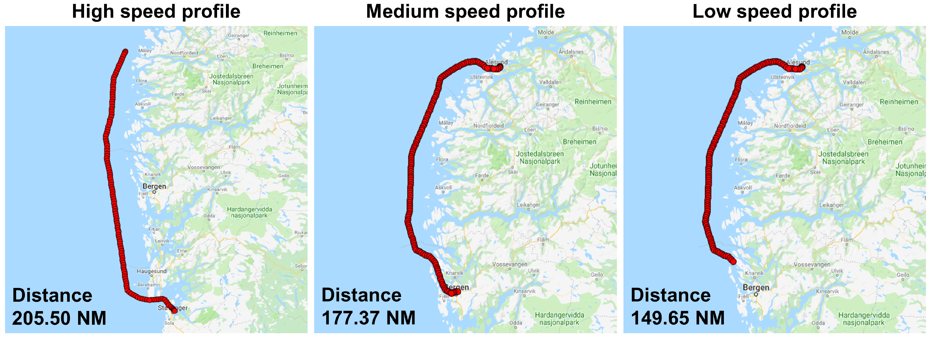
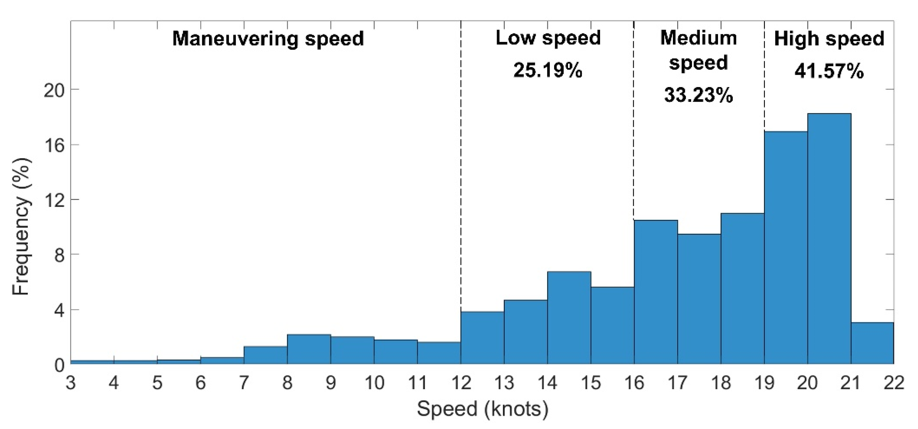
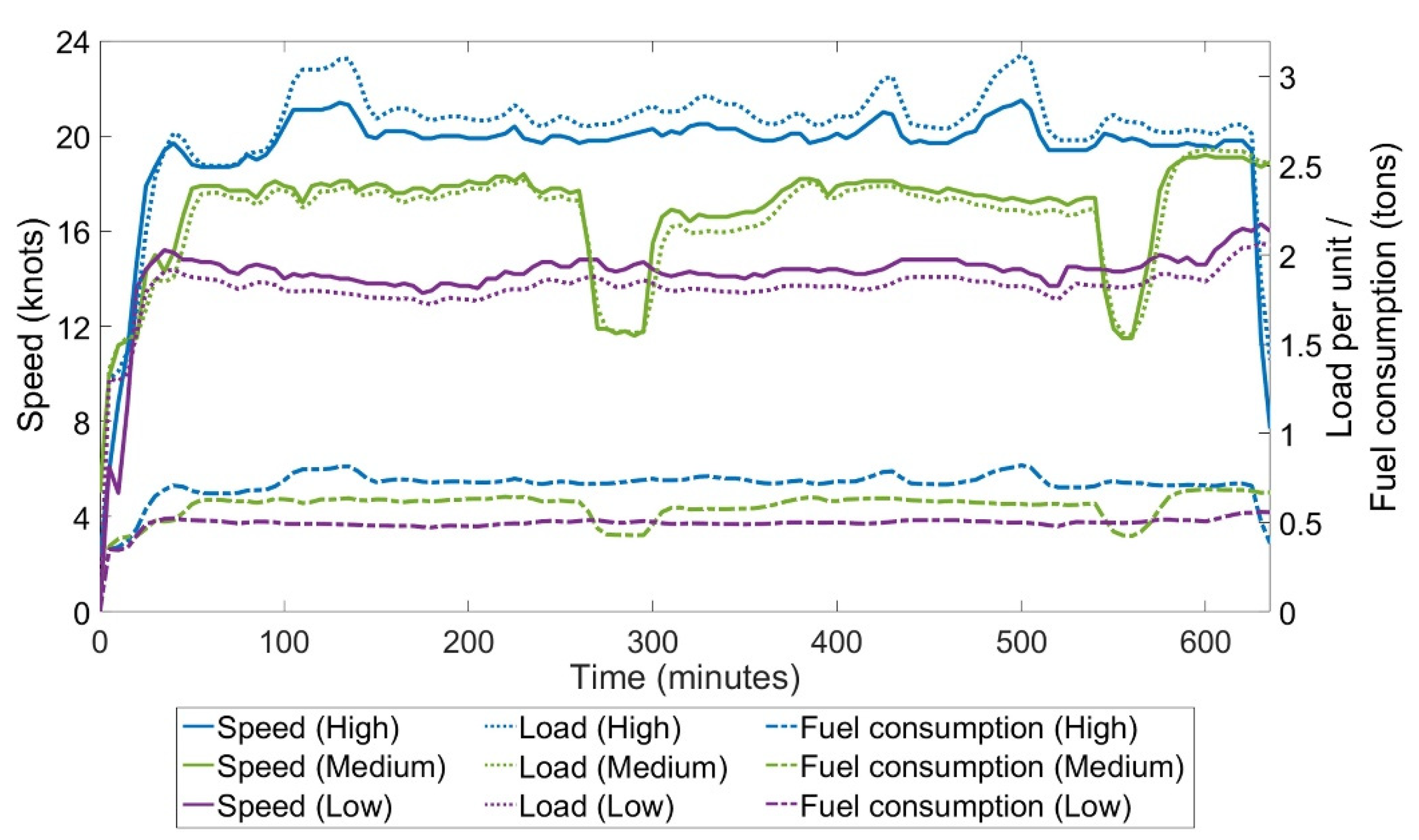
The determination of ship operation load profiles was based on actual voyages of the Britannia operating in the Norwegian Sea. The voyage data or baseline data was obtained from the Norwegian coastal authority and has been validated in [36]. The selected voyages were comprised of three scenarios: low-, medium- and high-speed profiles, as shown in Figure 5. The classification of the profiles was determined by the majority of speeds used; i.e., majorities of speeds between 12–15 knots, 16–18 knots and 19–21 knots were judged to be respectively low-, medium- and high-speed profiles, as classified with the contribution percentage in Figure 6. The baseline data of the profiles, consisting of cruising speed, load demands per unit and fuel consumption, are shown in Figure 7. For simplification, the “per unit” concept for system load demands and power generation (1 pu equals 16,800 kW) is used throughout this section.
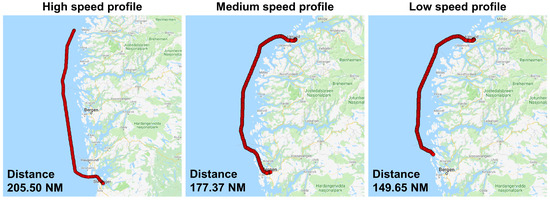
Figure 5.
Itineraries of the scenario profiles in the Norwegian Sea.

Figure 6.
Speed distribution and contributions of the Britannia.
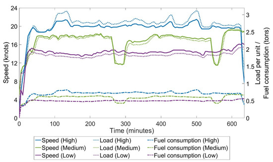
Figure 7.
Baseline data of all selected operation profiles.
The baseline fuel consumption was derived by establishing a conventional equal loading strategy, which evenly and proportionally distributed loads among all generators, as shown in Figure 8. Such symmetric load-sharing is recognized as the primary function of ship power management implemented on the majority of vessels. Thus, it could be assumed that the selected profiles were not optimized. Intelligent ship power management through a principle of asymmetric load-sharing and load-allocation optimization could then be applied to reschedule the operating states of engines. The various algorithms selected for the purpose of drawing performance comparisons included conventional techniques, like the constrained nonlinear multivariable function (FMINCON); well-known metaheuristics, like GA and PSO; and relatively novel metaheuristics, like grey wolf optimizer (GWO) and ant lion optimizer (ALO). An optimal solution was determined by the fitness value, which is the sum of the SFC derived from all active engine generators. The controlled parameters included maximum iterations of 200 and a population size defined as 10 times the number of dimensions. The parameter settings of all algorithms are summarized in Table 1. It can be noted that the WOA algorithm, along with the recently introduced GWO and ALO algorithms, offer a benefit in terms of immediate implementation, as they require no or very few parameters to be adjusted.
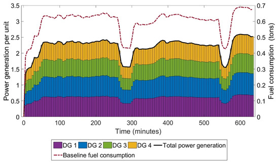
Figure 8.
Equal loading of generators and corresponding fuel consumption.

Table 1.
Parameter settings for the optimization algorithms.
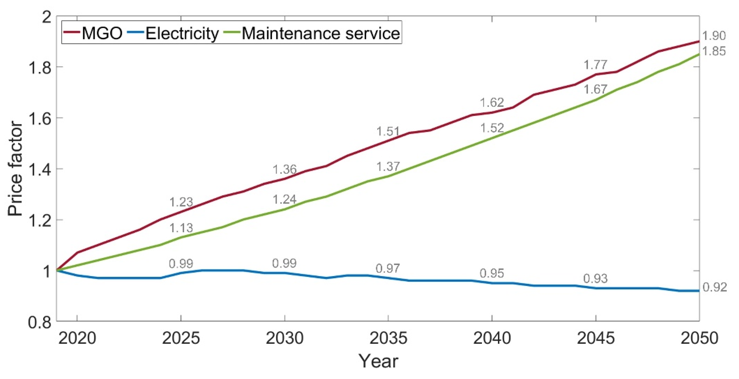
Next, the estimation of lifetime operation costs required assumptions and projections of parameter price scenarios throughout the ship operating period. By assuming a ship lifespan of 30 years, from 2021 to 2050, the forecasts of fuel oil and commercial electricity prices for the defined period could be derived from a recent energy outlook report [37], which provides petroleum price projections considering global economic growth and the introduction of renewable technologies. It was also assumed that the costs for maintenance and repair services would rise by approximately 2.0% annually [38]. The price trajectories for marine gas oil, shoreside electricity and maintenance services can then be converted to price factors over the ship lifetime, as shown in Figure 9. The estimation of annual fuel operation and upkeep service costs was based on the average ship cruising period of 14 hours/day and 350 days/year according to the itinerary information, while the estimation of port operating costs was based on the load demand and the time the ship spent at berth. According to a survey on engine load defaults for diesel-electric cruise vessels [39], the service load for berthing ships with a capacity range between 5500 to 6000 persons can be averaged at 14,000 kW. Finally, the average long-term discount rate of 2.05% was applied for the calculation of the values throughout the economic projection.
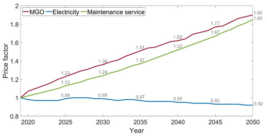
Figure 9.
Parameter price projections over the ship lifetime.
5.2. Fuel Operation Costs
The estimation of operating fuel consumption correlates closely with the function of ship power management through the optimization performance. The performance can be initially assessed by the trajectory of search agents, which should rapidly decline in the early stage and then gradually converge in order to guarantee a solution, as shown in Figure 10. At a load demand of 2.5 pu, the recent metaheuristics, including GWO, ALO and WOA, were able to find better solutions as compared to the GA and PSO, while the FMINCON was completely stuck in local optima. The excellence in convergence was probably due to a better balance between the global search (exploration) and local search (exploitation) that led to high local optima avoidance. The result also verified the competitiveness of the novel metaheuristics as compared to the prominent algorithms. The optimization performance was then further investigated by putting it into practice with a variation of loads from the selected profiles.
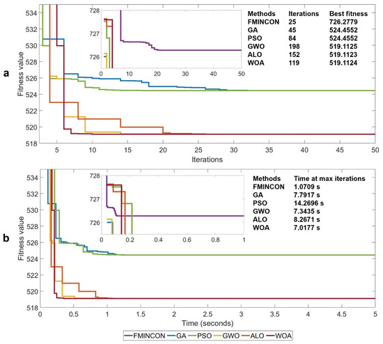
Figure 10.
Convergence characteristics of algorithms based on: (a) iterations (b) simulation time.
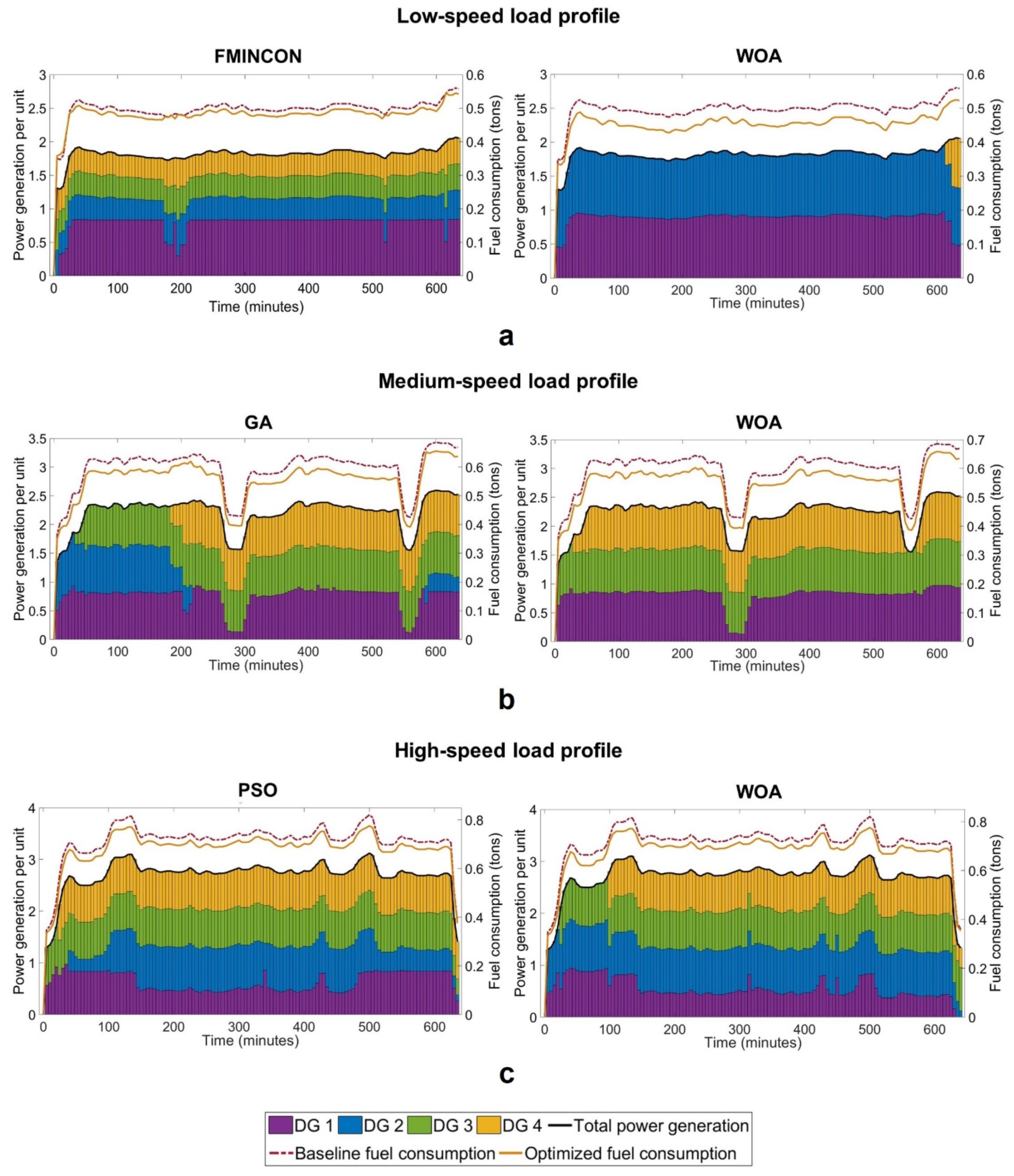
The load-dependent operating states of the established four DG system were optimally scheduled for low-, medium-, and high-speed profiles, as shown in Figure 11. At low-speed cruising, the FMINCON solution required all generators to be online, while only DG 1 enjoyed highly efficient operation and the rest of the DGs fell under suboptimal areas. On the other hand, the WOA solution allowed only two high-rating engines to operate at nearly full capacity, which could exceed an optimal SFC range. It turned out that such an optimized case was able to lower the engine fuel consumed. For the medium-speed profile, the GA solution unnecessarily switched on all generators for some operating points, leading to an increase in total fuel consumed. The WOA algorithm, on the other hand, allowed all active generators to function efficiently throughout the profile. In the high-speed scenario, all algorithms required every generator to be active when the load demand approached 3 pu. Each algorithm also demonstrated a variety of ways of assigning loads for individual components. Nevertheless, the loads had to surpass 3 pu to secure the optimum condition for the entire generation system.

Figure 11.
Comparison of optimization for the 4-DG system: (a) FMINCON and WOA with low-speed profile (b) GA and WOA with medium-speed profile (c) PSO and WOA with high-speed profile.
The optimal dispatch for the modified 5-DG configuration is shown in Figure 12. The assigned load conditions were different from those of the 4-DG system as two engines were replaced with three lower-rated ones. At low and medium speeds, for example, all active engines could efficiently run within their optimal ranges. This was due to a good match between the proposed engine capacities and the corresponding load demands. However, the optimal condition for the entire generation system was limited by high-speed load requirements, as one high-rating engine (DG 2 with the GWO) could not efficiently function for the most part except when exceeding 3 pu. In contrast, the optimization for the modified 6-DG system enabled all active generators to handle various load profiles more effectively through complementary operation of proper capacity engines, as shown in Figure 13. This also implied that the generation system design consisting of a greater quantity of smaller engine sizes tended to be more flexible and could cope with diverse load demands.
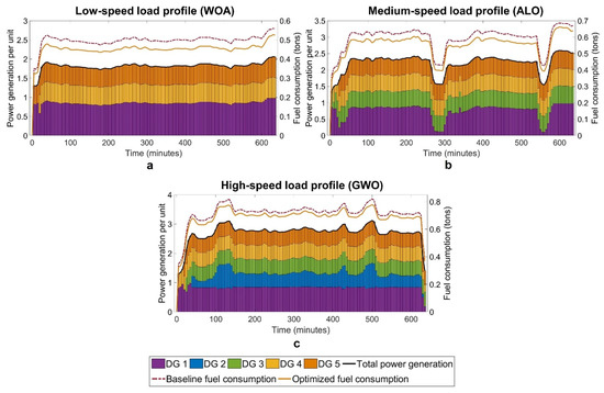
Figure 12.
Optimization of the 5-DG system by using novel algorithms: (a) WOA with low-speed profile (b) ALO with medium-speed profile (c) GWO with high-speed profile.
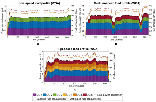
Figure 13.
Optimization of the 6-DG system by using WOA with: (a) low-speed profile (b) medium-speed profile (c) high-speed profile.
The optimal load assigned to individual engines can also be observed in the SFC map, as shown by comparing it with the symmetrical loading scheme in Figure 14. The metaheuristic attempt to minimize or eliminate inefficient working engine generators and distribute loads for the rest to the nearest possible energy-saving points was defined by an MCR of 80–90%. However, there were occasions when some engines were unable to operate within such an optimal condition due to a need to reduce or increase their carried loads and fill up the demand gap. Thus, they were placed within allowed loading ranges, usually between 60–80% or exceeding 90% of the MCR.
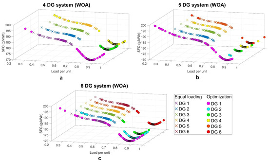
Figure 14.
SFC results for the medium-speed profile by using WOA with: (a) 4-DG system (b) 5-DG system (c) 6-DG system.
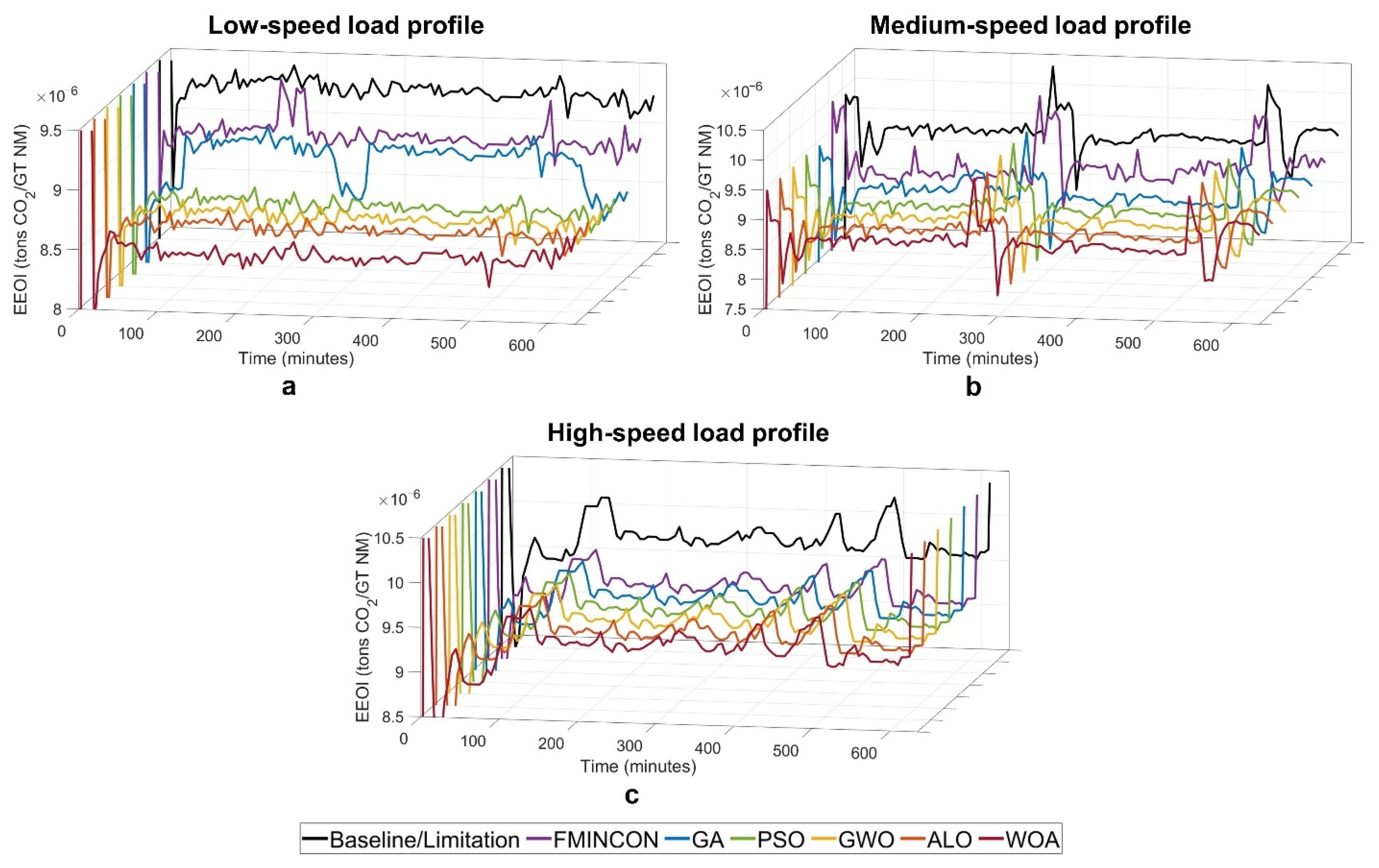
The emission abatement can be evaluated by the EEOI, which is not only used to monitor the GHG emissions, but also has a function as an operational constraint. It is apparent from Figure 15 that the EEOI results obtained from the optimization were maintained well below the EEOI baseline derived from the baseline fuel consumption over the entire operation range. At low speed, the WOA solution produced the lowest GHG emissions as a consequence of efficiently running with an optimal number of engines. Meanwhile, the FMINCON and GA demonstrated higher EEOI results due to prematurely falling into local optima, especially at low- and medium-speed profiles.
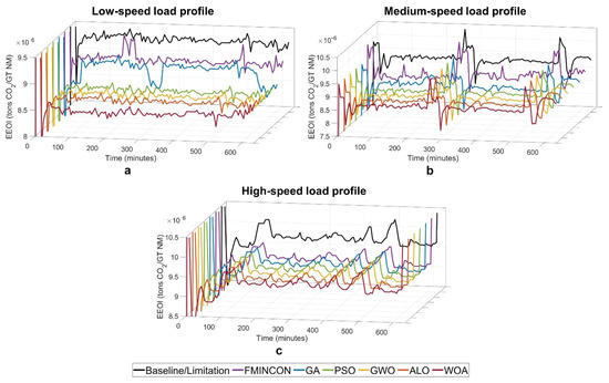
Figure 15.
EEOI profiles of the 4-DG system for (a) low-speed profile (b) medium-speed profile (c) high-speed profile.
The average fuel-saving for all algorithms is summarized in Table 2. The fuel-saving potential for the existing 4-DG architecture was estimated at 4.31–7.74%, varying with the profile, and could be further maximized by alternative plant designs for specific itinerary requirements. For example, the 5-DG system achieved the maximum fuel-saving of 8.86% when cruising at low speed, while the 6-DG system yielded a saving of 4.44% for the high-speed profile. It can be noted that the limited capacity to minimize fuel consumed in the course of rising loads was due to limited searching space for search agents. This meant that all generators tended to operate in the same manner with the equal loading scheme when the demand approached the maximum limit of generation capability.
Table 2.
Average fuel-saving results of all algorithms.
With respect to the optimization performance, all recent metaheuristics in general provided better solutions compared to the classical or conventional metaheuristic techniques, though the proposed WOA algorithm was able to achieve the best solutions in almost cases. Whale optimization-based ship power management was thus selected for the cost estimation procedure as it proved to be the most efficient means to deal with various load profiles. However, it should be noted that there was no algorithm that achieved superior results for all optimization challenges. In other words, a particular metaheuristic solution, like the WOA, that comes up with very promising solutions for this problem may not be suited for many others, in the sense that there is no free lunch (NFL) in a search [40].
The result of average fuel-saving can then be used to estimate the annual fuel cost-saving and the reduction in emissions, as exemplified for the 4-DG system in Table 3. The estimation also took into account the contribution of speed profiles; i.e., the amount of fuel consumed was proportional to the ship speed distribution as a percentage. A reduction in combustion emissions can be measured by the multiplication of the reduced fuel consumption and associated emission factors. By deploying the load allocation scheme in the considered Britannia-class vessel, as much as USD1,635,924 could be saved in the annual fuel expenditure and a CO2 emissions reduction of 6807 tons could be achieved.
Table 3.
Average fuel-saving results of all algorithms.
5.3. Maintenance Service Costs
The unscheduled maintenance or repair service costs are likely to vary depending on the reliability of the system architecture. A simple reliability assessment can be carried out on the basis of the N + X topology using k-out-of-n parallel elements, as summarized in Table 4. It is evident that, if the number of active generators is equal to the number of installed generators (n-out-of-n), the system is viewed as a series configuration and thus perceived to have low reliability. Conversely, the system reliability can be improved by incorporating a simple parallel, i.e., a system that remains operational with the smallest number of active generators (1-out-of-n). A higher level of reliability also indicates sufficient generation capacity to support the load if one or more units fail. The 6-DG system, for example, ensures a maximum reliability of 99.65% when relying on two active generators at partial load conditions. Should one of the generators fail, there will be four additional generators available to deliver the same generation capacity as originally intended. However, such an arrangement may experience the worst reliability when the system tends toward a series configuration at the maximum load demand.
Table 4.
Reliability for N + X redundancy systems.
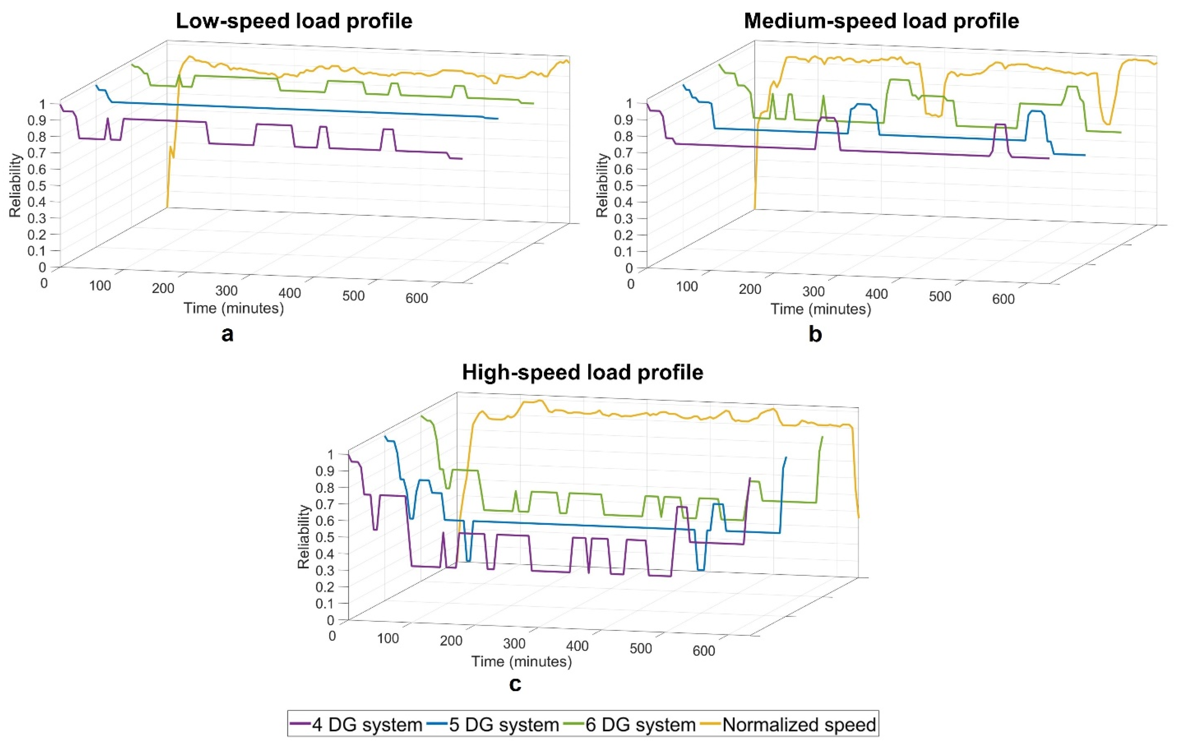
For non-homogeneous component systems, the reliability was assessed using weighted k-out-of-n redundancy, as shown in Table 5. The evaluation was based on the classification of weight factors and consideration of all possible events for which the total generation capacity must be at least the specified threshold. The ship power management is then responsible for determining an optimum event in tandem with optimally allocating loads to minimize fuel consumed. The reliability profiles of architecture when initiating the evaluation scheme can be observed in Figure 16. The 4-DG system periodically suffered being from the least reliable design as a consequence of fewer backup generators being available. However, the system ensured the highest degree of reliability on average for all profiles. In contrast, the 5- and 6-DG system designs seemed to show greater dependability improvements due to implementing greater quantities of components; however, they nonetheless entailed a higher chance of failure as a consequence of introducing more complex failure modes into the system.
Table 5.
Reliability for weighted k-out-of-n redundancy systems.
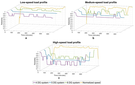
Figure 16.
Reliability profiles of configurations for: (a) low-speed profile (b) medium-speed profile (c) high-speed profile.
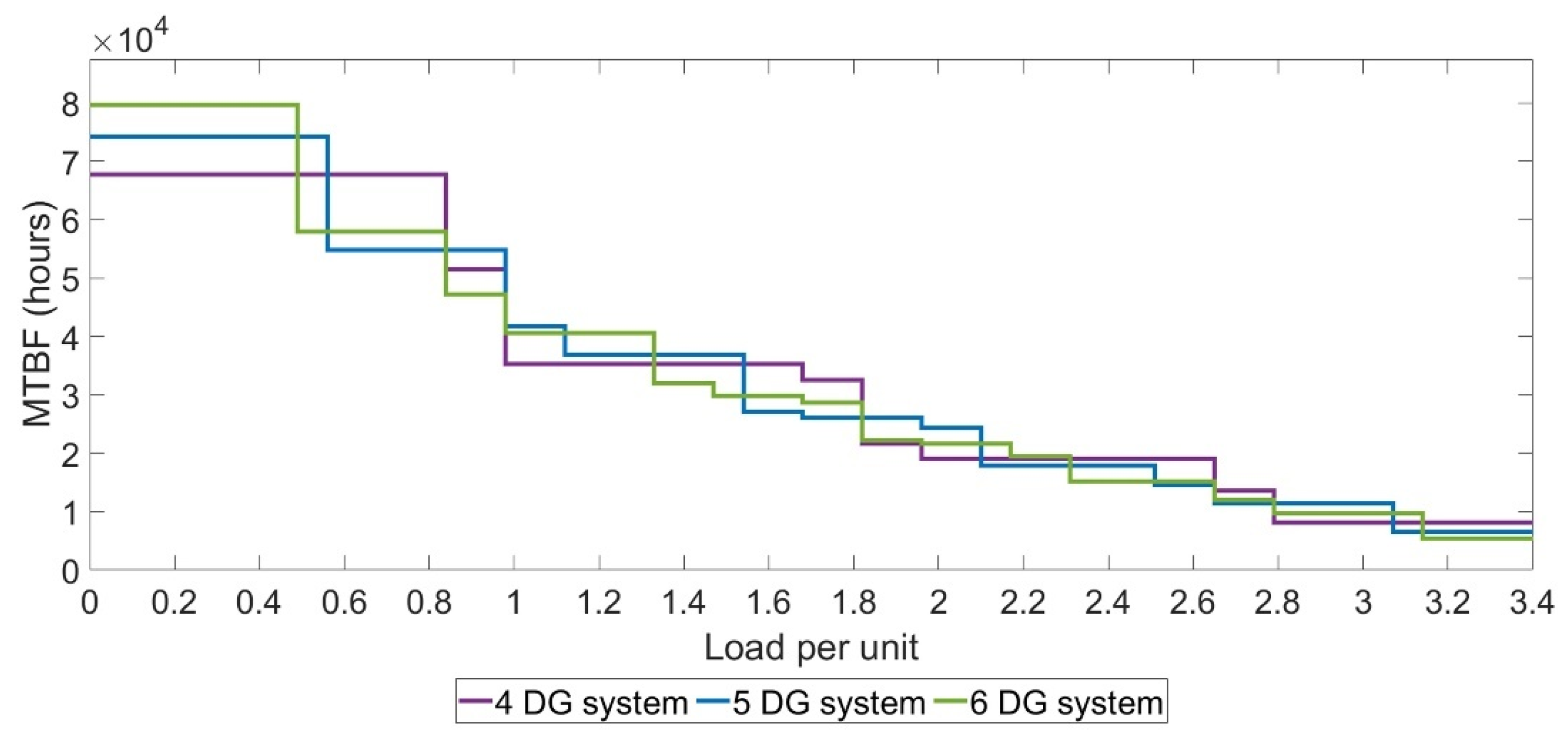
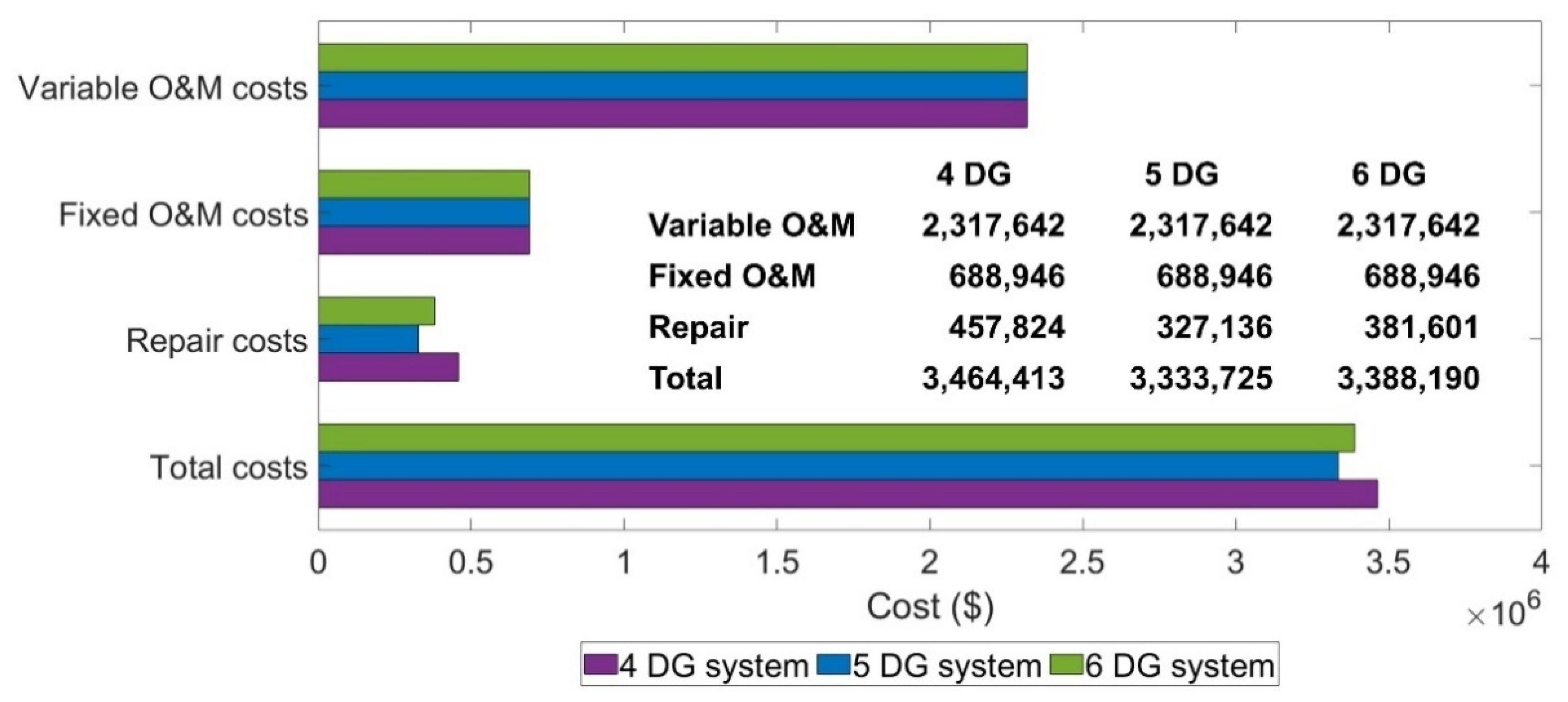
According to Equations (13)–(15), the variables related to the upkeep service are composed of power capacity, energy demands and system failure characteristics. Reliability improvement through the modification of system redundancy therefore represents an alternative approach for controlling ship operation costs. Figure 17 shows the system MTBF extracted from the weighted k-out-of-n redundancy used for the estimation of repair expenditure. The derived MTBF was inversely correlated with the load applied, as a reduction in system redundancy in the course of rising loads means boosting a chance of failure. Figure 18 gives a detailed cost breakdown of consolidated maintenance for a 3 pu load. It can be noticed that the repair costs are correlated with the reliability value obtained in Table 5, according to which the most reliable system proves to be that with the most economic design with regard to maintenance expenditure.

Figure 17.
Extracted system MTBF of conventional configurations compared with load demands.
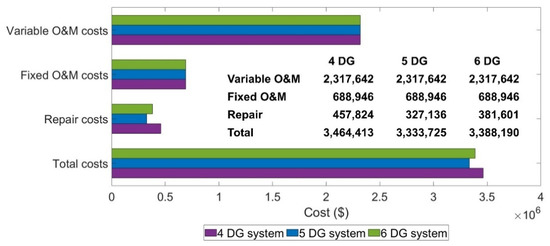
Figure 18.
Annual maintenance service costs breakdown at a 3 pu load.
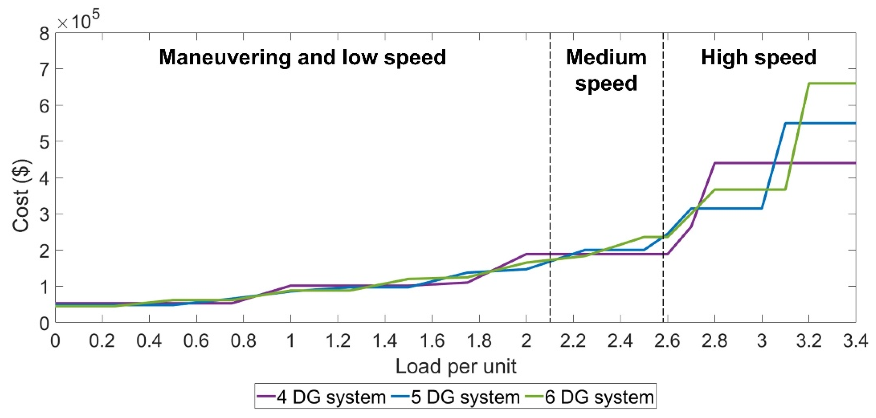
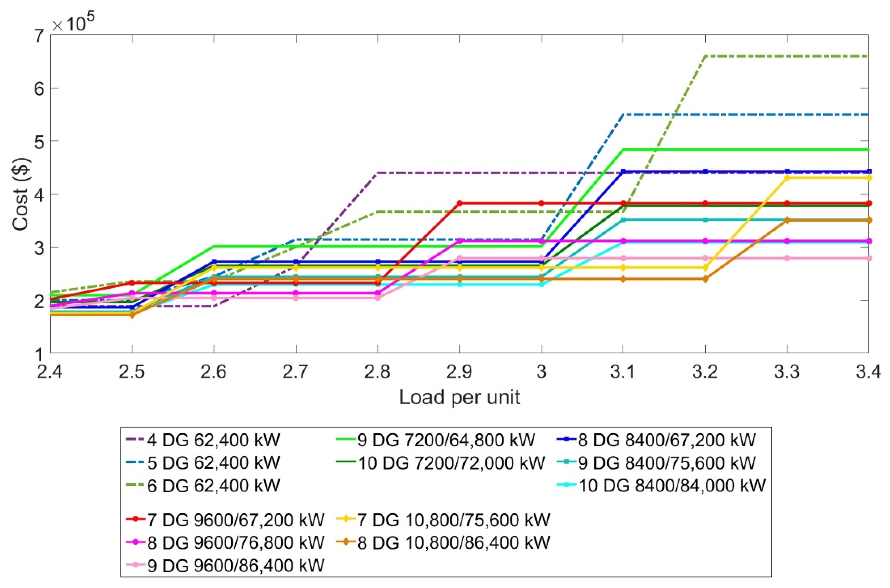
When taking all load scenarios into consideration, the repair costs respond accordingly to increasing load demands, most notably within the high-speed area, as shown in Figure 19. Each architecture offers a minimum cost for specific load ranges. For instance, the 4-DG arrangement provides the lowest repair costs if the average ship loading is between 2.3 and 2.7 pu or above 3.1 pu, while the 5-DG is the most cost-effective design within the load range of 2.8 to 3 pu.
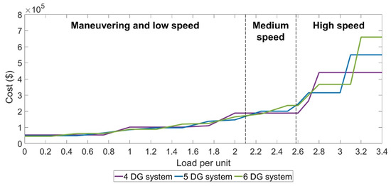
Figure 19.
Annual repair costs of conventional configurations compared to load demands.
A significant increase in the repair costs under high load conditions poses a challenge for the cruise line industry in working towards a solution to minimize such expenditure. This study introduced non-conventional parallel system designs that could minimize whole-life operation costs by maximizing system trustworthiness throughout all operating ranges. The proposed systems were composed of L-type engines with capacities varying from 7200 kW to 10,800 kW and also involved expanding power generation capacities from 62,400 kW to 86,400 kW, as detailed in Table 6. The selected engines could be organized into non-conventional arrangements, i.e., installation of more than six prime movers, which is rarely seen in the majority of cruise vessels. For the requirement of extending system capacity, the plant project cost per unit of installed power should be taken into consideration. The project cost basically consists of the installation cost and the costs of the generator set package plus auxiliary equipment, like heat recovery and exhaust gas treatment systems. The total cost then can be minimized on the basis of N + X parallel redundancy as follows:
Table 6.
Non-conventional system designs with average fuel-saving results.
The estimation of annual repair service costs for all proposed configurations is shown in Figure 20. The majority of non-conventional designs clearly demonstrate their high levels of reliability, represented by the suppression of repair costs in spite of entering the high load area. It can also be observed that the systems with greater power production tend to keep costs down with increasing load demands. Such non-conventional designs, however, may be subject to an increase in fixed O&M costs as a result of increasing generation capacity, as shown in Figure 21. This indicates the significance of determining appropriate installed power for the requirement of lowering the total maintenance and repair services costs.
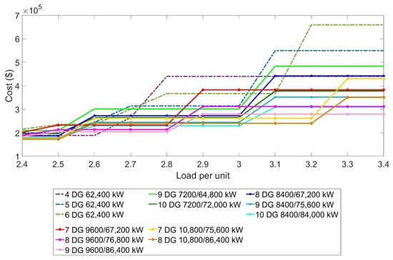
Figure 20.
Annual repair costs of all configurations with high load demands.
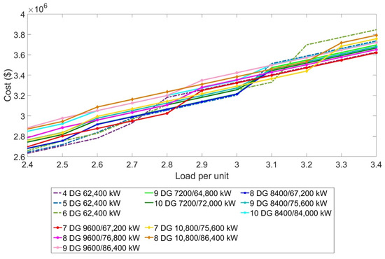
Figure 21.
Total annual maintenance and repair costs of all configurations.
5.4. Decision-Making Process on Power Plant System Design
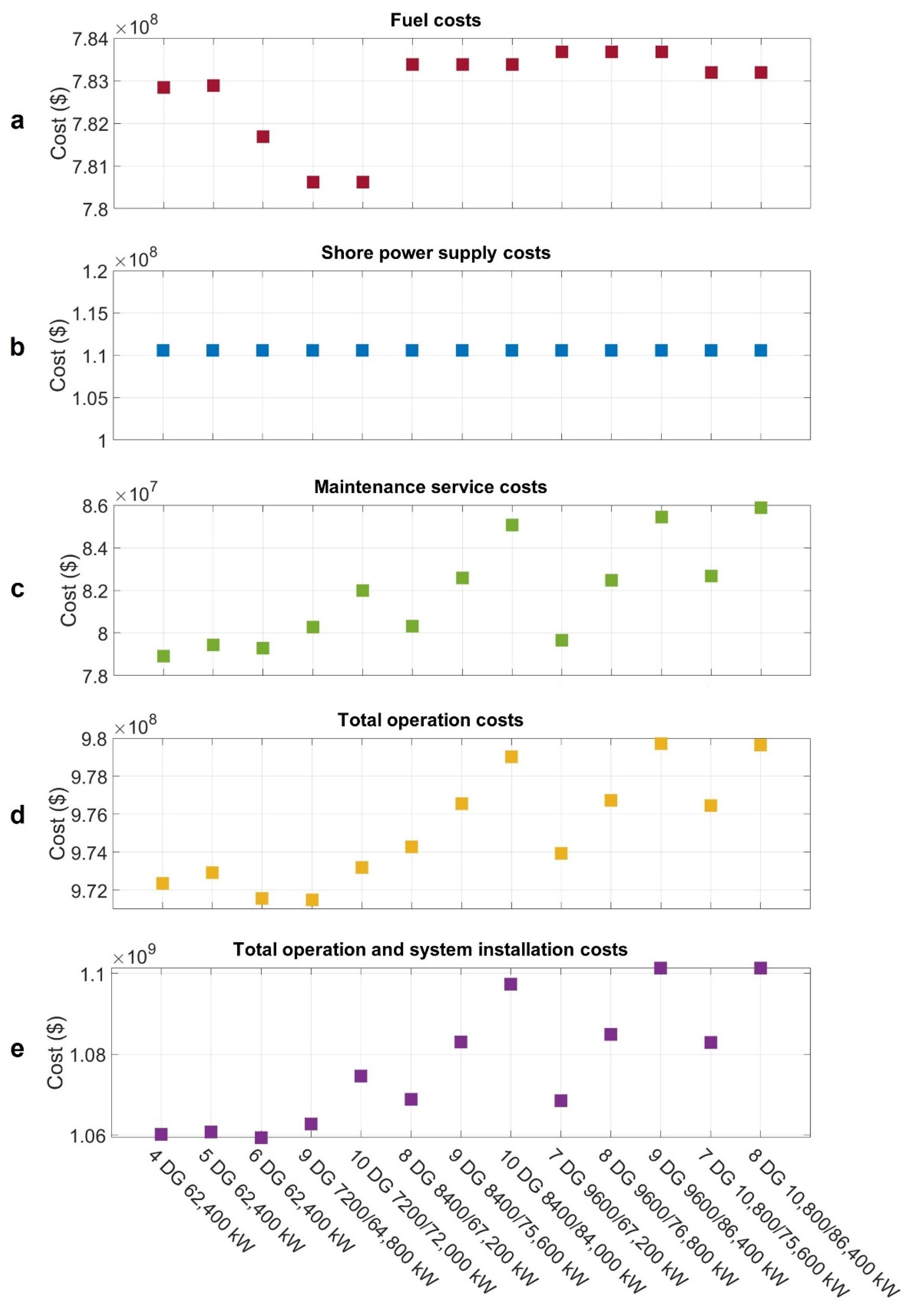
The main concern of holistic cost-effective design is that of incorporating all economic-related components, as shown in Figure 22. The lifetime fuel operation costs were based on the average fuel-saving results derived from Table 2 and Table 6. An appropriate power plant design can be initially determined from frequent ship speed ranges and the corresponding fuel consumed. Generally, cruise ships operating in open seas use medium and high speeds for the majority of cruising time. The non-conventional 9-DG7200/64,800 kW and 10-DG 7200/72,000 kW system designs, which provided significant fuel savings for such speeds, would therefore have secure cruising operations, with a minimum fuel consumption of USD780,615,529 over the ship lifetime.
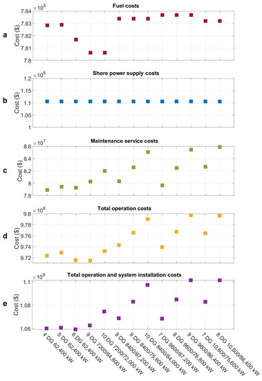
Figure 22.
Lifetime cost components of all configuration designs: (a) fuel costs (b) shore power supply costs (c) maintenance service costs (d) total operation costs (e) total operation and system installation costs.
The total operation costs are also partly accounted for by energy demands at ports, represented by shoreside electricity supply costs. However, such costs are entirely dependent on hotel service machinery, regardless of power generation sources, as generators need to be shut down during the period. The value of lifetime power supply costs of USD110,587,138, derived from the average port operation demand, was hence applied for all configuration designs.
The requirement for the minimum maintenance deals with a compromise between system reliability and complexity. A system consisting of a greater quantity of components may end up less reliable due to introducing more complex failure modes, whereas lowering the quantity could reduce its reliability due to fewer available backup options. There is also a need for compromise for conflicting service cost components. The conventional designs experienced escalating repair costs with the rise of load demands. On the contrary, the parallel designs with extended capacity were capable of bringing such costs down but this proved a hindrance due to the prohibitive costs of scheduled maintenance. The conventional 4-DG, which was able to keep the total costs to a minimum of USD78,910,423, therefore represents an optimum balance between incurred potential costs.
There is also a trade-off between operating cost requirements, as the reliability advantage from one system design may be outweighed by more economic and environmental benefits obtained from the other designs. The consolidation of cost components hence results in a solution for the selection of system architecture. The non-conventional 9-DG7200/64,800 kW proved to be an alternative system design for the requirement of minimizing ship operating costs. The system secured the whole-life costs at a minimum of USD971,478,589, mainly due to its superiority in optimizing load allocation. This means that, even though the maintenance expense of the system cannot be reduced to a minimum, the total operation costs can be diminished eventually through a considerable saving in fuel expenditure. However, this does not necessarily mean initiatives to improve system reliability can be disregarded, as the safety of ships and passengers, as well as consequent downtime costs associated with system failure, are also important.
Finally, the initial investment can be taken into account to facilitate a comparison between systems with various capacities. The 6-DG configuration, which achieved an overall lifetime cost of USD1,059,413,775, was the ultimate solution design when considering the comprehensive cost components. The minimum cost obtained also emphasized the potential of holistic design to meet industrial needs. In the competitive context of the cruising industry, an approach that is able to identify optimal power plants across several architecture choices hence came up with a solution for cruise lines to survive in the market. In summary, the holistic design seeks an optimum balance between fuel efficiency, reliability and system capacity in compliance with environmental constraints. The determination of capacity should be based on the requirement of minimizing capital investment, while the optimal arrangement should be able to significantly reduce fuel consumed and maintenance service costs across a variety of load profiles.
6. Conclusions
A holistic approach to determining optimal system design from economic and environmental perspectives was herein developed. Lifetime operation costs are very dependent on optimized load allocation and system design structure. Metaheuristic algorithms were introduced into the ship power management case study to determine the optimum use of installed systems onboard, whereas reliability design was applied to determine the maintenance. Alternative configurations with both conventional and non-conventional designs were assessed through fuel operation, shore electricity and maintenance service, as well as investment expenditure.
The main conclusions of this study can be summarized as follows:
- The optimal dispatch using the WOA ensured minimum GHG emissions and fuel operation expenses through elimination of inefficient working engines and by optimally distributing loads to the rest of the working generators. The algorithm was able to reduce fuel consumption by a range of 4.04–8.86%, varying with the profiles and configurations. The system with a greater quantity of components appeared to be more elastic and was able to cope with diverse load profiles thanks to complementary operation of smaller displacement engines. However, the utilization of such engine sizes may suffer from lower efficiency, as evidenced by their SFC characteristics.
- The reliability design is usually a trade-off between the repair service and overall expenditure. The conventional designs bore escalating failure costs during high-load demands, whereas the unconstrained capacity systems ensured additional resilience. However, such highly reliable designs may be hindered by the costliness of the starting capital and scheduled maintenance.
- The holistic design seeks a compromise solution for contradictory cost requirements. The most reliable system may be outweighed by more fuel-efficient designs in the sense of minimizing ship operating costs, while the most cost-effective design in terms of system costs may vary depending on the generation capacity. Proper consideration at the design stage is therefore necessary to determine which power plant architecture is most likely to offer a clear advantage in fulfilling specific requirements of the vessel.
Energy efficiency requirements in the context of maritime regulations are becoming even more stringent. As required by the IMO, a 30% reduction in GHG emissions released is mandated for all applicable ships from 2025 onwards. Hence, integration of energy storage technology for large diesel-electric ships and the application of forthcoming metaheuristics for next-generation ship power management could be introduced in future research work. Such a concept of system design not only further reduces fuel consumption and emissions, but ensures even an higher level of electrical system reliability.
Author Contributions
Conceptualization, C.N. and T.L.; methodology, C.N. and H.X.; software, C.N.; investigation, C.N. and H.X.; writing—original draft, C.N.; writing—review & editing, T.L.; supervision, T.L. All authors have read and agreed to the published version of the manuscript.
Funding
This work was supported by the Research on the Mid-Sized Cruise Ship Development (G18473CZ04) in the High-Tech Ships R&D Program of MIIT China.
Institutional Review Board Statement
Not applicable.
Informed Consent Statement
Not applicable.
Data Availability Statement
Not applicable.
Acknowledgments
The authors would like to thank all colleagues in the Large Engine Research Center of NAOCE. The first author gratefully acknowledges the support from the China Scholarship Council.
Conflicts of Interest
The authors declare no conflict of interest.
Nomenclature
| CF | fuel mass to CO2 mass conversion factor (ton CO2/ton fuel) |
| Celectricity | electricity price (USD/kWh) |
| Cfixed O&M | fixed operation and maintenance cost (USD/kW-year) |
| Cfuel | marine gas oil price (USD/ton) |
| Crepair | repair cost (USD/kW/h) |
| Csystem | system cost (USD/kW) |
| Cvariable O&M | variable operation and maintenance cost (USD/kWh) |
| EF | emission factor (ton/ton fuel) |
| e | substance of emission |
| FC | mass of consumed fuel (tons) |
| f | fuel type |
| g | engine type |
| k | required number of operating generators |
| L | ship lifespan (years) |
| n | number of installed generators |
| P | instantaneous power (kW) |
| Ptotal | total power demand (pu) |
| pj | power assigned to jth engine (pu) |
| R | reliability value |
| Rstart-up | maximum allowed load increase rate (pu) |
| Rup/down | maximum permissible instant load step (pu) |
| r | discount rate (%) |
| Thorizon | cruising time period |
| V | ship speed (knots) |
| w | weight value |
| Δt | time interval |
| λ | failure rate (failures/year) |
| μ | repair rate (repairs/year) |
| Abbreviations | |
| ALO | ant lion optimizer |
| CGS | classifier-guided sampling |
| DG | diesel generator |
| DP | dynamic programming |
| ECA | emission control area |
| EEOI | energy efficiency operational indicator |
| FMINCON | constrained nonlinear multivariable function |
| GA | genetic algorithm |
| GHG | greenhouse gas |
| GT | gross tonnage |
| GWO | grey wolf optimizer |
| IMO | International Maritime Organization |
| KPI | key performance indicator |
| LCC | life cycle cost |
| MCR | maximum continuous rating |
| MGO | marine gas oil |
| MTBF | mean time between failures |
| MTTF | mean time to failure |
| MTTR | mean time to repair |
| NFL | no free lunch |
| NSGA-II | non-dominated sorting genetic algorithm II |
| O&M | operation and maintenance |
| PSO | particle swarm optimization |
| SFC | specific fuel consumption |
| SQP | sequential quadratic programming |
| SSE | sum of squared estimate of errors |
| WOA | whale optimization algorithm |
Appendix A
Table A1.
Parameters for the Britannia-class vessel.
Table A1.
Parameters for the Britannia-class vessel.
| General characteristics | ||||
| Tonnage | 143,730 GT | Delivery | 2015 | |
| Length overall | 330 m | Speed | 21.9 knots | |
| Beam moulded | 38.38 m | Maximum capacity | 5722 persons | |
| Design draught | 8.55 m | Classification society | Lloyd’s Register | |
| Power system configuration | ||||
| Propulsion | Diesel-electric propulsion system 2xVEM Sachsenwerk propulsion motors Total propulsion power 36,000 kW | |||
| Power generation | 2xWärtsilä 14V46F and 2xWärtsilä 12V46F Total generated power 62,400 kW, 60 Hz, at 514 rpm Alternator efficiency 0.976 | |||
| Configuration design | 4-DG system (existing) | 5-DG system | 6-DG system | |
| Prime mover | DG 1 DG 2 DG 3 DG 4 DG 5 DG 6 | 14V46F/16,800 kW 14V46F/16,800 kW 12V46F/14,400 kW 12V46F/14,400 kW | 14V46F/16,800 kW 14V46F/16,800 kW 8L46F/9600 kW 8L46F/9600 kW 8L46F/9600 kW | 12V46F/14,400 kW 12V46F/14,400 kW 7L46F/8400 kW 7L46F/8400 kW 7L46F/8400 kW 7L46F/8400 kW |
| Emission data [28] | ||||
| Operation area | Emission control area (ECA) | |||
| Emission standards | IMO NOX emission tier III | |||
| Fuel type | Marine gas oil (MGO) with 0.1% sulphur content | |||
| CO2 emission factor | 3.206 CO2 ton/ton fuel | |||
| Reliability data [29] | ||||
| Reliability parameter | Failure rate (failures/year) | Mean time between failure MTBF (hours) | Mean time to repair MTTR (hours) | |
| Diesel engine | 0.1003 | 87,337.98 | 4.06 | |
| Engine-driven generator | 0.1691 | 51,803.67 | 32.70 | |
| Diesel generator | 0.2694 | 32,516.70 | 10.34 | |
| Economic data [41,42,43] | ||||
| Generator set package | USD575/kW | Variable O&M (service) | USD0.0075/kWh | |
| Heat recovery system | USD175/kW | Variable O&M (consumable) | USD0.0010/kWh | |
| Exhaust gas treatment | USD150/kW | Total variable O&M cost Cvariable O&M | USD0.0085/kWh | |
| Installation | USD508/kW | Repair cost Crepair | USD1.0889/kW/h | |
| Total system cost Csystem | USD1408/kW | MGO price Cfuel | USD698.50/ton | |
| Fixed O&M cost Cfixed O&M | USD10/kW-year | Electricity price Celectricity | USD0.1052/kWh | |
| Algorithm A1. Pseudo-code of the whale optimization algorithms (WOA). |
| Initialize the whale population Xi (i = 1, 2, …, n) |
| Calculate the fitness of search agent: X* = the best search agent |
| while (t < maximum number of iterations) |
| for each search agent: Update a, A, C, l and p |
| if 1 (p < 0.5) |
| if 2 ( < 1): Update position of search agents by: |
| else if 2 ( ≥ 1): Select a random search agent (Xrand) |
| Update position of search agents by: |
| end if 2 |
| else if 1 (p ≥ 0.5): Update position of search agents by: |
| end if 1 |
| end for |
| Calculate the fitness of search agent: Update X* for a better solution |
| t = t + 1 |
| end while |
| Return X* |
References
- IMO. MEPC 75/7/15 Reduction of GHG Emissions from Ship Fourth IMO GHG Study 2020; International Maritime Organization: London, UK, 2020. [Google Scholar]
- Vergara, J.; McKesson, C.; Walczak, M. Sustainable energy for the marine sector. Energy Policy 2012, 49, 333–345. [Google Scholar] [CrossRef]
- Bouman, E.A.; Lindstad, E.; Rialland, A.I.; Strømman, A.H. State-of-the-art technologies, measures, and potential for reducing GHG emissions from shipping—A review. Trans. Res. D Trans. Environ. 2017, 52, 408–421. [Google Scholar] [CrossRef]
- Geertsma, R.D.; Negenborn, R.R.; Visser, K.; Hopman, J.J. Design and control of hybrid power and propulsion systems for smart ships: A review of developments. Appl. Energy 2017, 194, 30–54. [Google Scholar] [CrossRef]
- Nuchturee, C.; Li, T.; Xia, H. Energy efficiency of integrated electric propulsion for ships–A review. Renew. Sustain. Energy Rev. 2020, 134, 110145. [Google Scholar] [CrossRef]
- Allianz. Safety and Shipping Review 2019 an Annual Review of Trends and Developments in Shipping Losses and Safety; Allianz Global Corporate & Specialty: Munich, Germany, 2019. [Google Scholar]
- Kanellos, F.D.; Tsekouras, G.J.; Hatziargyriou, N.D. Optimal demand-side management and power generation scheduling in an all-electric ship. IEEE Trans. Sustain. Energy 2014, 5, 1166–1175. [Google Scholar] [CrossRef]
- Michalopoulos, P.; Kanellos, F.D.; Tsekouras, G.J.; Prousalidis, J.M. A method for optimal operation of complex ship power systems employing shaft electric machines. IEEE Trans. Transp. Electr. 2016, 2, 547–557. [Google Scholar] [CrossRef]
- Baldi, F.; Ahlgren, F.; Melino, F.; Gabrielii, C.; Andersson, K. Optimal load allocation of complex ship power plants. Energy Convers. Manag. 2016, 124, 344–356. [Google Scholar] [CrossRef]
- Ancona, M.A.; Baldi, F.; Bianchi, M.; Branchini, L.; Melino, F.; Peretto, A.; Rosati, J. Efficiency improvement on a cruise ship: Load allocation optimization. Energy Convers. Manag. 2018, 164, 42–58. [Google Scholar] [CrossRef]
- Sakalis, G.N.; Frangopoulos, C.A. Intertemporal optimization of synthesis, design and operation of integrated energy systems of ships: General method and application on a system with Diesel main engines. Appl. Energy 2018, 226, 991–1008. [Google Scholar] [CrossRef]
- Kanellos, F.D.; Anvari-Moghaddam, A.; Guerrero, J.M. A cost-effective and emission-aware power management system for ships with integrated full electric propulsion. Electr. Power Syst. Res. 2017, 150, 63–75. [Google Scholar] [CrossRef] [Green Version]
- Huang, Y.; Lan, H.; Hong, Y.Y.; Wen, S.; Fang, S. Joint voyage scheduling and economic dispatch for all-electric ships with virtual energy storage systems. Energy 2020, 190, 116268. [Google Scholar] [CrossRef]
- Pradhan, M.; Roy, P.K.; Pal, T. Grey wolf optimization applied to economic load dispatch problems. Int. J. Electr. Power Energy 2016, 83, 325–334. [Google Scholar] [CrossRef]
- Sulligoi, G.; Vicenzutti, A.; Menis, R. All-electric ship design: From electrical propulsion to integrated electrical and electronic power systems. IEEE Trans. Transp. Electr. 2016, 2, 507–521. [Google Scholar] [CrossRef]
- Vicenzutti, A.; Menis, R.; Sulligoi, G. All-electric ship-integrated power systems: Dependable design based on fault tree analysis and dynamic modeling. IEEE Trans. Transp. Electr. 2019, 5, 812–827. [Google Scholar] [CrossRef]
- Backlund, P.B.; Seepersad, C.C.; Kiehne, T.M. All-electric ship energy system design using classifier-guided sampling. IEEE Trans. Transp. Electr. 2015, 1, 77–85. [Google Scholar] [CrossRef]
- Jeong, B.; Wang, H.; Oguz, E.; Zhou, P. An effective framework for life cycle and cost assessment for marine vessels aiming to select optimal propulsion systems. J. Clean. Prod. 2018, 187, 111–130. [Google Scholar] [CrossRef] [Green Version]
- Zhu, J.; Chen, L.; Wang, B.; Xia, L. Optimal design of a hybrid electric propulsive system for an anchor handling tug supply vessel. Appl. Energy 2018, 226, 423–436. [Google Scholar] [CrossRef]
- Zhu, J.; Chen, L.; Wang, X.; Yu, L. Bi-level optimal sizing and energy management of hybrid electric propulsion systems. Appl. Energy 2020, 260, 114134. [Google Scholar] [CrossRef]
- Trivyza, N.L.; Rentizelas, A.; Theotokatos, G. A novel multi-objective decision support method for ship energy systems synthesis to enhance sustainability. Energy Convers. Manag. 2018, 168, 128–149. [Google Scholar] [CrossRef] [Green Version]
- Trivyza, N.L.; Rentizelas, A.; Theotokatos, G. Impact of carbon pricing on the cruise ship energy systems optimal configuration. Energy 2019, 175, 952–966. [Google Scholar] [CrossRef] [Green Version]
- Bolbot, V.; Trivyza, N.L.; Theotokatos, G.; Boulougouris, E.; Rentizelas, A.; Vassalos, D. Cruise ships power plant optimisation and comparative analysis. Energy 2020, 196, 117061. [Google Scholar] [CrossRef]
- Balland, O.; Erikstad, S.O.; Fagerholt, K. Concurrent design of vessel machinery system and air emission controls to meet future air emissions regulations. Ocean. Eng. 2014, 84, 283–292. [Google Scholar] [CrossRef]
- Hebner, R.E.; Uriarte, F.M.; Kwasinski, A.; Gattozzi, A.L.; Estes, H.B.; Anwar, A.; Cairoli, P.; Dougal, R.A.; Feng, X.; Chou, H.; et al. Technical cross-fertilization between terrestrial microgrids and ship power systems. J. Mod. Power Syst. Clean Energy 2016, 4, 161–179. [Google Scholar] [CrossRef] [Green Version]
- Lloyd’s Register. Rules and Regulations for the Classification of Ships; Lloyd’s Register Group Limited: London, UK, 2019. [Google Scholar]
- IMO. MEPC.1/Circ.684 Guidelines for Voluntary Use of the Ship Energy Efficiency Operational Indicator (EEOI); International Maritime Organization: London, UK, 2009. [Google Scholar]
- Smith, T.W.; Jalkanen, J.P.; Anderson, B.A.; Corbett, J.J.; Faber, J.; Hanayama, S.; Pandey, A. Third IMO Greenhouse Gas Study 2014; International Maritime Organization: London, UK, 2014. [Google Scholar]
- IEEE. Recommended Practice for the Design of Reliable Industrial and Commercial Power Systems; IEEE Inc.: New York, NY, USA, 2007. [Google Scholar]
- Stevens, B.; Dubey, A.; Santoso, S. On improving reliability of shipboard power system. IEEE Trans. Power Syst. 2014, 30, 1905–1912. [Google Scholar] [CrossRef]
- Wu, J.S.; Chen, R.J. An algorithm for computing the reliability of weighted-k-out-of-n systems. IEEE Trans. Reliab. 1994, 43, 327–328. [Google Scholar]
- Eryilmaz, S.; Sarikaya, K. Modeling and analysis of weighted-k-out-of-n: G system consisting of two different types of components. Proc. Inst. Mech. Eng. O J. Risk. Reliab. 2014, 228, 265–271. [Google Scholar] [CrossRef]
- Wärtsilä. Wärtsilä 46F Product Guides; Wärtsilä Corporation: Helsinki, Finland, 2017. [Google Scholar]
- Mirjalili, S.; Lewis, A. The whale optimization algorithm. Adv. Eng. Softw. 2016, 95, 51–67. [Google Scholar] [CrossRef]
- Gharehchopogh, F.S.; Gholizadeh, H. A comprehensive survey: Whale Optimization Algorithm and its applications. Swarm Evol. Comput. 2019, 48, 1–24. [Google Scholar] [CrossRef]
- Simonsen, M.; Walnum, H.; Gössling, S. Model for estimation of fuel consumption of cruise ships. Energies 2018, 11, 1059. [Google Scholar] [CrossRef] [Green Version]
- U.S. EIA. Annual Energy Outlook 2020 with Projections to 2050; U.S. Energy Information Administration: Washington, DC, USA, 2020. [Google Scholar]
- Moore Stephens. Future Operating Costs Report; Moore Stephens LLP: London, UK, 2018. [Google Scholar]
- Agrawal, A.; Aldrete, G.; Anderson, B.; Muller, R.; Ray, J. Port of Los Angeles Inventory of Air Emissions–2016; Starcrest Consulting Group LLC: Albuquerque, NM, USA, 2017. [Google Scholar]
- Wolpert, D.H.; Macready, W.G. No free lunch theorems for optimization. IEEE Trans. Evol. Comput. 1997, 1, 67–82. [Google Scholar] [CrossRef] [Green Version]
- Darrow, K.; Tidball, R.; Wang, J.; Hampson, A. Catalog of CHP Technologies; U.S. Environmental Protection Agency and the U.S. Department of Energy: Washington, DC, USA, 2017. [Google Scholar]
- Lazard. Levelized Cost of Energy Analysis—Version 11.0. Available online: https://www.lazard.com/media/450337/lazard-levelized-cost-of-energy-version-110.pdf (accessed on 18 May 2021).
- AECOM. Spon’s Mechanical and Electrical Services Price Book; CRC Press: Boca Raton, FL, USA, 2018. [Google Scholar]


Publisher’s Note: MDPI stays neutral with regard to jurisdictional claims in published maps and institutional affiliations. |
© 2021 by the authors. Licensee MDPI, Basel, Switzerland. This article is an open access article distributed under the terms and conditions of the Creative Commons Attribution (CC BY) license (https://creativecommons.org/licenses/by/4.0/).