The Price Difference and Trend Analysis of Yesso Scallop (Patinopecten yessoensis) in Changhai County, China

Abstract

This paper focuses on the difference in inter-group and intra-group price of Yesso scallop (Patinopecten yessoensis) and the simulation accuracy of three different exponential smoothing models in the price. Based on the farm-gate price and wholesale price data of P. yessoensis in Changhai county from January 2017 to December 2018, this study uses the Wilcoxon rank sum test to compare the inter- and intra-group price and applies simple exponential smoothing (SES), Holt’s linear trend method, and Holt-Winters’ additive method to simulate and predict the price. The results suggest that (i) to improve economic benefits, it is necessary to formulate reasonable farming area and establish low-density ecological cultivation mode; (ii) the price’s Akaike information criterion (AIC) and mean absolute percentage error (MAPE) values by the SES model are optimal, and the MAPE value is lower than 4%; and (iii) the result of SES analysis shows no obvious change from January to March 2019.

1. Introduction

According to data from the FishStatJ database [1], China’s scallop production in 1979 was only 180 metric tons (t), accounting for less than 1% of world scallop production. In 2017, the country’s scallop production soared to 2 million t, accounting for approximately 72% of the world’s total. The above data show that the scale of China’s scallop industry has continued to expand. The national scallop industry plays a significant role in promoting fisheries economic growth in coastal regions, and it has produced enormous socioeconomic and ecological benefits [2,3,4,5].

At present, Chinese native scallop species mainly include Chlamys farreri and Chlamys nobilis, and the introduced species are Argopecten irradians and Patinopecten yessoensis [6]. Due to the large size and rapid growth of Yesso scallop (Patinopecten yessoensis), it has become a species with high economic value in Chinese scallop mariculture [7]. P. yessoensis is a cold-watered bivalve shellfish native to northern Japan and Russian Far East coastal waters [8,9]. Since the introduction of P. yessoensis from Japan, the research and promotion of Chinese researchers for many years has broken through key technologies (e.g., artificial seedling, intermediate breeding, proliferation, aquaculture, etc.), and P. yessoensis has increased in scale and industrialization in the northern Yellow Sea in China [10].

However, due to a lack of aquaculture planning and irregular production mode, the mortality of P. yessoensis increased in the Changhai county, China [11,12]. This affects the production and quality of P. yessoensis and may cause abnormal fluctuation in the farm-gate price and wholesale price. It can damage the interests of aquaculture producers and endanger the sustainable development of the industry. This paper aims to investigate the difference in inter- and intra-group price of P. yessoensis and simulate the price trend.

Many researchers have conducted the method innovations on the prediction of aquatic product prices and proposed a variety of prediction methods in different contexts. There are two main categories: (1) There is a widely used time series model (see, e.g., [13,14,15,16,17,18]) which applies the autoregressive moving average models and error correction model to analyze various aquatic product prices. Zhang and Yang (2018) applied the Holt-Winters model to simulate shrimp wholesale prices [19]. He et al. (2010) and Li et al. (2014) predicted fish wholesale prices through the neural network method [20,21]. Purcell et al. (2018) studied the market price of beche-de-mer by applying a regression model [22]. (2) In addition, there is a predictive model of several method combinations; for example, Zhang et al. (2005) constructed an aquatic product price forecasting support system, integrated neural network, moving average, linear regression, and other models to study price data [23]. Garza-Gil et al. (2009) used the linear, semi-log, double-log, and quadratic models to predict the aquaculture production and price trends of sea bream, sea bass, and turbot in Spain [24]. Zhou et al. (2017) introduced the consumer price index and applied the catastrophic grey model to conduct risk warning research on oyster prices [25].

There are numerous studies on the law of price fluctuation. In China’s aquatic products market, the price fluctuation may bring huge uncertainty to the income of aquaculture producers and operators [26]. Based on the autoregressive conditional heteroskedasticity model, a series of studies believed that the price fluctuation of aquatic products has the characteristics of clustering, no memory, high risk, and high payback [27,28]. Nguyen et al. (2013) estimated the demand for crustaceans in the United States retail stores, and results indicate that shrimp demand has price elasticity, while that of the crab, crawfish, and lobster is inelastic [29]. Asche et al. (2015) explored the price volatility regimes using the FAO Fish Price Index and they found that the price volatility of aquaculture products is much lower than that of wild products [30]. Some studies indicate that the price fluctuation has a diffusion effect through the investigated characteristics of price fluctuation in the aquatic product market [31,32].

Other research involves market integration and price transmission of aquatic products. For example, Hoshino et al. (2015) examined the price dynamics of imported abalone in Japan [33], Wakamatsu and Miyata (2015) surveyed the demand for the Japanese cod market [34], Singh (2016) explored the price transmission between different imported Atlantic salmon products in the United States market [35], and some researchers studied the price transmission of export chains and/or value chains [36,37,38,39].

In summary, the price difference of aquatic products is relatively less concerned. The price difference and trend predicting model for P. yessoensis would assist aquaculture producers to make reasonable farming area and density and improve farm management. This paper aims to better understand the price difference of P. yessoensis and predict future prices. In the study, a non-parametric method is introduced to measure the difference in the inter- and intra-group price of P. yessoensis, and three different exponential smoothing models are used to simulate the farm-gate price and wholesale price to determine the optimal prediction model.

The remainder of the paper is as follows: Section 2 describes data sources and methods, Section 3 shows the results, and Section 4 discusses and summarizes the paper.

2. Materials and Methods

2.1. Data Sources

The farming of P. yessoensis in China is mainly distributed in the coastal areas of the Liaoning and Shandong provinces, among which the farming in Liaoning province is concentrated in the waters around Changhai county [11,12]. To facilitate the research, this paper selects the price of P. yessoensis produced in Zhangzidao and Haiyangdao in this county as the research object. The location of price data collection in this paper is shown in Figure 1.

Data are from the molluscan shellfish industry in China Modern Agro-industry Technology Research System (CARS). The CARS has set up some price-monitoring stations for shellfish products in China. The research period is from January 2017 to December 2018. This paper uses two-year price data, mainly because it is difficult to collect price data; moreover, this study focuses on the price difference and short-term trend simulation, so short data series are sufficient for analysis.

In this paper, the farm-gate price refers to the price of P. yessoensis produced in Zhangzidao (ZZ) and Haiyangdao (HY); it is divided into extra large (EL), large (L), medium (M), small (S), and extra small (ES) by specification (

Table 1. Specification description in farm-gate price.

Specification	Code	The Number of Scallops per Kilogram (kg)
Extra Large	EL	4–5
Large	L	6–8
Middle	M	9–10
Small	S	11–12
Extra Small	ES	13–16

). The wholesale price refers to the market price in Beijing (BJ), Guangzhou (GZ), Shenzhen (SZ), Changsha (CS), Harbin (HR), Changchun (CC), Shenyang (SY), Shanghai (SH), Hangzhou (HZ), Chengdu (CD), Hefei (HF), Ningbo (NB), and Xiamen (XM) (

Table 2. Source and market description in wholesale price.

Market Name	Code	Source
		ZZ	HY
Beijing	BJ	EL, L, M, S, ES	EL, L, M, S, ES
Guangzhou	GZ	EL, L, M, S, ES	EL, L, M, S, ES
Shenzhen	SZ	L, M, S, ES	L, M, S, ES
Changsha	CS	S, ES	S, ES
Harbin	HR	S, ES	S, ES
Changchun	CC	S, ES	S, ES
Shenyang	SY	S, ES	S, ES
Shanghai	SH	S, ES	ES
Hangzhou	HZ	S, ES	ES
Chengdu	CD	S, ES	ES
Hefei	HF	S, ES	ES
Ningbo	NB	S, ES	ES
Xiamen	XM	S, ES	—

Note: Source refers to the specification in each market is from the Zhangzidao (ZZ) group or Haiyangdao (HY) group. The farm-gate group includes Zhangzidao (ZZ) and Haiyangdao (HY); the market group includes Beijing (BJ), Guangzhou (GZ), Shenzhen (SZ), Changsha (CS), Harbin (HR), Changchun (CC), Shenyang (SY), Shanghai (SH), Hangzhou (HZ), Chengdu (CD), Hefei (HF), Ningbo (NB), and Xiamen (XM); the same below.

). The unit is Chinese Yuan per kilogram (CNY per kg). Figure 2 shows the explanation of each group. Figure 3 presents the boxplot of price series with minimum, lower quartile (25th percentile), median (50th percentile), upper quartile (75th percentile), and maximum.

2.2. Methodology

This study assumes that for the P. yessoensis in Zhangzidao and Haiyangdao, the farming company’s production technology and consumer preference for scallop demand remain unchanged or change little.

2.2.1. Non-Parametric Test

There are two reasons for using the non-parametric method. First, the price is independent between the farm-gate and each wholesale market, so the Wilcoxon rank sum test is used to compare the inter- and intra-group price [40,41]. Second, we applied the adjustment method proposed to control the overall type I error rate to a large extent [42]. This study uses the test from [43] to compare the difference in the inter-group (source and specification) and intra-group (farm-gate and wholesale market) price of the P. yessoensis. The advantage of this method is that under the premise of controlling the probability of making a type I error, pairwise comparison between all groups can be performed simultaneously. The calculation process is completed by R software.

2.2.2. Exponential Smoothing Models

Exponential smoothing models are a common method for predicting future values of time series, and it has been proved that their short-term prediction ability is better than long-term prediction ability [44,45,46]. Therefore, this paper uses simple (single) exponential smoothing (SES), Holt’s linear trend method, and Holt-Winters’ additive method to simulate the farm-gate price and wholesale price. The three models are tested and compared by the Akaike information criterion (AIC) [47,48] and mean absolute percentage error (MAPE). The optimal model is selected to make a short-term prediction of the price. The calculation process is completed by R software’s forecast package.

The formulas of the three models are as follows:

(i) Simple exponential smoothing:

$$\{\begin{array}{l}{S}_t=\alpha x_t+(1-\alpha )S_{t-1}\\ y_{t+1}=S_t\end{array}$$

(1)

(ii) Holt’s linear trend method:

$$\{\begin{array}{l}{S}_t=\alpha x_t+(1-\alpha )(S_{t-1}+b_{t-1})\\ b_t=\beta (S_t-S_{t-1})+(1-\beta )b_{t-1}\\ y_{t+k}=S_t+b_{t}k\end{array}$$

(2)

(iii) Holt-Winters’ additive method:

$$\{\begin{array}{l}{S}_t=\alpha (x_t-I_{t-m})+(1-\alpha )(S_{t-1}+b_{t-1})\\ b_t=\beta (S_t-S_{t-1})+(1-\beta )b{}_{t-1}\\ I_t=\gamma (x_t-S_{t-1}-b_{t-1})+(1-\gamma )I_{t-m}\\ y_{t+k}=S_t+b_{t}k+I_{t+k-m}\end{array}$$

(3)

where S_t, b_t, and I_t are the estimate of the level (smoothed value), trend (slope), and season of the series at time t, respectively; α, β, and γ are the smoothing parameter for the level, trend, and season, respectively; x_t and y_t+k are the actual value and simulated value, respectively; m is the length of the season (the number of month or season); and k is the step-ahead forecast.

The AIC and MAPE calculation processes are as follows:

(iv) AIC:

$$AIC=2n-2\ln (L)$$

(4)

where n is the number of the parameter and L is the likelihood function.

(v) MAPE:

$$MAPE=\frac{1}{s}{\displaystyle \sum _{t=1}^s\frac{\left|y_t-x_t\right|}{x_t}}$$

(5)

where s is the sample size and x_t and y_t are the actual value and simulated value of the price data, respectively.

3. Results

3.1. Difference Comparison

3.1.1. Inter-Group Difference

Table 3. The differences between sources in the farm-gate group and the wholesale market group.

Name	Group.1	Group.2	W-Stat	p-Value
Farm-gate (n = 240)	HY	ZZ	7064.5	0.8006
BJ (n = 240)	HY	ZZ	7035	0.7584
GZ (n = 240)	HY	ZZ	6746	0.3976
SZ (n = 192)	HY	ZZ	4332	0.4725
CS (n = 96)	HY	ZZ	1092.5	0.6535
HR (n = 96)	HY	ZZ	1230.5	0.5589
CC (n = 96)	HY	ZZ	1233.5	0.5480
SY (n = 96)	HY	ZZ	1230.5	0.5589
SH (n = 48)	HY	ZZ	257.5	0.5272
HZ (n = 48)	HY	ZZ	307.5	0.6924
CD (n = 48)	ZZ	HY	212.5	0.1131
HF (n = 48)	HY	ZZ	288	1.0000
NB (n = 48)	HY	ZZ	288	1.0000

shows the test result of sources and

Table 4. The differences between specifications in the farm-gate group and the wholesale market group.

Name	Group.1	Group.2	W-Stat
Farm-gate (n = 240)	ES	S	268
	ES	M	6
	ES	L	0
	ES	EL	0
	S	M	145
	S	L	0
	S	EL	0
	M	L	238
	M	EL	0
	L	EL	161
BJ (n = 240)	ES	S	560
	ES	M	26
	ES	L	0
	ES	EL	0
	S	M	300
	S	L	0
	S	EL	0
	M	L	458
	M	EL	33
	L	EL	348
GZ (n = 240)	ES	S	374
	ES	M	12
	ES	L	0
	ES	EL	0
	S	M	185
	S	L	0
	S	EL	0
	M	L	291
	M	EL	0
	L	EL	214
SZ (n = 192)	ES	S	374
	ES	M	12
	ES	L	0
	S	M	185
	S	L	0
	M	L	291
CS (n = 96)	ES	S	540
HR (n = 96)	ES	S	560
CC (n = 96)	ES	S	470
SY (n = 96)	ES	S	560

Note: All p-values here are lower than 0.001 (0.1% significance level), so they are omitted.

shows the significant test result of specifications (EL, L, M, S, and ES). The result of Table 3 indicates that there is no statistically significant difference in sources (p > 0.1), while that of Table 4 has a statistically significant difference in specifications and all significance at the level of 0.1% (p < 0.001).

3.1.2. Intra-Group Difference

Table 5. The differences between ZZ and wholesale markets and between the wholesale markets in the ZZ group.

Name	Group.1	Group.2	W-Stat	p-Value
EL (n = 72)	ZZ	BJ	91	0.0000 ****
	ZZ	GZ	25.5	0.0000 ****
	BJ	GZ	206.5	0.0601 *
L (n = 96)	ZZ	BJ	146	0.0100 **
	ZZ	GZ	64	0.0000 ****
	ZZ	SZ	64	0.0000 ****
M (n = 96)	ZZ	BJ	146	0.0100 **
	ZZ	GZ	64	0.0000 ****
	ZZ	SZ	64	0.0000 ****
S (n = 336)	ZZ	XM	100.5	0.0085 ***
	ZZ	GZ	108	0.0140 **
	ZZ	SZ	108	0.0140 **
ES (n = 336)	ZZ	HZ	129.5	0.0873 *
	ZZ	SH	129.5	0.0873 *
	ZZ	HF	129.5	0.0873 *
	ZZ	CC	129.5	0.0873 *
	ZZ	NB	129.5	0.0873 *
	ZZ	CS	104.5	0.0111 **
	ZZ	GZ	104.5	0.0111 **
	ZZ	SZ	104.5	0.0111 **
	ZZ	XM	79.5	0.0014 ***

Note: *, **, ***, and **** indicate significance at the levels of 10%, 5%, 1%, and 0.1%, respectively; the same below.

and

Table 6. The differences between HY and wholesale markets and between the wholesale markets in the HY group.

Name	Group.1	Group.2	W-Stat	p-Value
EL (n = 72)	HY	BJ	146	0.0050 ***
	HY	GZ	95	0.0002 ****
L (n = 96)	HY	BJ	146	0.0100 **
	HY	GZ	95	0.0003 ****
	HY	SZ	95	0.0003 ****
M (n = 96)	HY	BJ	179	0.0902 *
	HY	GZ	161	0.0487 **
	HY	SZ	161	0.0487 **
ES (n = 312)	HY	BJ	133	0.0712 *
	HY	HR	133	0.0712 *
	HY	SY	133	0.0712 *
	HY	CC	99	0.0057 ***
	HY	CD	99	0.0057 ***
	HY	GZ	99	0.0057 ***
	HY	SZ	99	0.0057 ***
	HY	CS	72	0.0003 ****

Note: *, **, ***, and **** indicate significance at the levels of 10%, 5%, 1%, and 0.1%, respectively; the same below.

show the significant test results of the ZZ and wholesale market and the HY and wholesale market, respectively. In terms of the number of pairwise comparisons with statistically significant difference and their proportion in the total pairwise comparison, in the ZZ group, the number of the EL, L, M, S, and ES specifications are 3, 3, 3, 3, and 9 pairs, respectively, while the proportion of the above specifications are 3/3, 3/6, 3/6, 3/91, and 9/91, respectively. In the HY group, the number of the above specifications are 2, 3, 3, 0, and 8 pairs, respectively, while the proportion of the above specifications are 2/3, 3/6, 3/6, 0/28, and 8/78, respectively.

3.2. Price Simulation

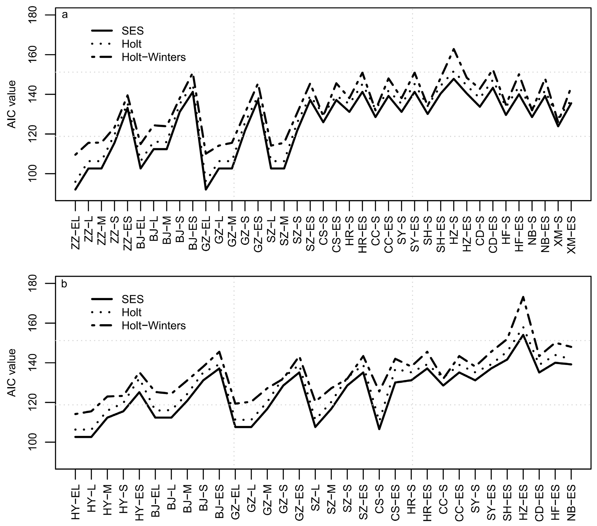
3.2.1. Model Selection

Figure 4 and Figure 5 show the AIC and MAPE value, respectively. It can be clearly seen that the AIC values of the SES model in Figure 4 is the lowest of the three models. The MAPE values of the SES model in the ZZ group are the smallest of the three models (MAPE value < 3%) (Figure 5a); except for the HY-ES, CS-S, and CS-ES specification in the HY group, the MAPE values of the remaining specification in SES model is also the lowest (MAPE value < 4%) (Figure 5b). Specifically, in the 39 sets of data series in the ZZ group, the MAPE value of 24 sets is lower than 2%; in the 32 sets of data series in the HY group, the MAPE value of 18 sets does not exceed 2%. Therefore, the SES model is selected to simulate the farm-gate price and wholesale price of P. yessoensis.

3.2.2. Simulated Results

The actual value and simulated value in the ZZ group (Figure 6) and in the HY group (Figure 7) from January 2017 to December 2018. It can be seen from the figures that the farm-gate and wholesale prices show obvious seasonal fluctuations, which are between December and February of the following year. This period coincides with China’s Spring Festival. This paper predicts the farm-gate price and wholesale price in the ZZ group (

Table 7. The predicted value of each specification price in the ZZ group (CNY per kg).

Time	ZZ-EL	ZZ-L	ZZ-M	ZZ-S	ZZ-ES	BJ-EL	BJ-L	BJ-M	BJ-S	BJ-ES
Jan-19	68.000	64.000	60.000	48.001	40.003	72.000	68.000	64.000	50.001	42.001
Feb-19	68.000	64.000	60.000	48.001	40.003	72.000	68.000	64.000	50.001	42.001
Mar-19	68.000	64.000	60.000	48.001	40.003	72.000	68.000	64.000	50.001	42.001
Time	GZ-EL	GZ-L	GZ-M	GZ-S	GZ-ES	SZ-L	SZ-M	SZ-S	SZ-ES	CS-S
Jan-19	72.000	68.000	64.000	50.001	42.002	68.000	64.000	50.001	42.002	50.002
Feb-19	72.000	68.000	64.000	50.001	42.002	68.000	64.000	50.001	42.002	50.002
Mar-19	72.000	68.000	64.000	50.001	42.002	68.000	64.000	50.001	42.002	50.002
Time	CS-ES	HR-S	HR-ES	CC-S	CC-ES	SY-S	SY-ES	SH-S	SH-ES	HZ-S
Jan-19	42.002	50.001	42.001	50.002	42.004	50.001	42.001	50.001	42.002	42.011
Feb-19	42.002	50.001	42.001	50.002	42.004	50.001	42.001	50.001	42.002	42.011
Mar-19	42.002	50.001	42.001	50.002	42.004	50.001	42.001	50.001	42.002	42.011
Time	HZ-ES	CD-S	CD-ES	HF-S	HF-ES	NB-S	NB-ES	XM-S	XM-ES
Jan-19	42.002	50.002	42.003	50.001	42.003	50.002	42.004	50.001	42.019
Feb-19	42.002	50.002	42.003	50.001	42.003	50.002	42.004	50.001	42.019
Mar-19	42.002	50.002	42.003	50.001	42.003	50.002	42.004	50.001	42.019

) and the HY group (

Table 8. The predicted value of each specification price in the HY group (CNY per kg).

Time	HY-EL	HY-L	HY-M	HY-S	HY-ES	BJ-EL	BJ-L	BJ-M	BJ-S	BJ-ES
Jan-19	68.000	64.000	60.000	48.001	47.167	72.000	68.000	64.000	50.001	42.002
Feb-19	68.000	64.000	60.000	48.001	47.167	72.000	68.000	64.000	50.001	42.002
Mar-19	68.000	64.000	60.000	48.001	47.167	72.000	68.000	64.000	50.001	42.002
Time	GZ-EL	GZ-L	GZ-M	GZ-S	GZ-ES	SZ-L	SZ-M	SZ-S	SZ-ES	CS-S
Jan-19	72.000	68.000	64.000	50.002	42.001	68.000	64.000	50.002	42.001	52.500
Feb-19	72.000	68.000	64.000	50.002	42.001	68.000	64.000	50.002	42.001	52.500
Mar-19	72.000	68.000	64.000	50.002	42.001	68.000	64.000	50.002	42.001	52.500
Time	CS-ES	HR-S	HR-ES	CC-S	CC-ES	SY-S	SY-ES	SH-ES	HZ-ES	CD-ES
Jan-19	51.084	50.001	42.002	50.002	42.001	50.001	42.002	42.002	42.003	42.001
Feb-19	51.084	50.001	42.002	50.002	42.001	50.001	42.002	42.002	42.003	42.001
Mar-19	51.084	50.001	42.002	50.002	42.001	50.001	42.002	42.002	42.003	42.001
Time	HF-ES	NB-S
Jan-19	42.003	42.004
Feb-19	42.003	42.004
Mar-19	42.003	42.004

) from January to March 2019. The results demonstrate that the price has not fluctuated during this period, and will continue to maintain the previous price. The results may ignore the seasonal influence to a certain extent, and a more detailed discussion will follow.

4. Discussion and Conclusions

4.1. Discussion

According to the difference comparison results, the differences between sources are not obvious; however, the differences between specifications are obvious. For the proportion in the total pairwise comparison, the significant difference of a larger size (EL, L, and M) was greater than that of a smaller size (S and ES). The difference is mainly in the specification, which may be because the geographical location and environmental condition of Zhangzidao and Haiyangdao are roughly the same [11]. Therefore, the influence of the source on the price is not significant. Some studies indicate that the average shell height of high-density cultivation was lower than that of low-density cultivation and the cumulative mortality rate of high-density cultivation was greater than that of low-density cultivation [49,50]. The differences between specifications under different cultivation densities are significant, which leads to different prices. These results are consistent with our finding.

According to the simulating results, the AIC and MAPE values of the SES model are optimal in the three models, and the MAPE value in the ZZ group and HY group are both not more than 4%. The farm-gate price and wholesale price remain the previous price from January to March 2019. The MAPE value of ES specification in the ZZ group and HY group simulated by the Holt model and of the HZ-S specification in the ZZ group and of the HZ-ES specification in the HY group simulated by the Holt-Winters model are larger; however, the price simulations of the other specifications are better for the two models. This also indicates that there are trend terms and/or seasonal terms in the price series, but the impacts of the trend and seasonal factors on the price are not obvious, which may be due to the short time scale of the price series. This requires continuous monitoring of the farm-gate price and wholesale price, and the updated data are supplemented to the model to make the prediction more accurate. Consistent with previous results [13,14,19], the price of P. yessoensis and other aquatic products have the same characteristics. That is, the supply of P. yessoensis is affected by the farming cycle and the instability of supply will cause the random fluctuation of price.

The hypothesis mentioned earlier in this paper is that from the collected price data, the price change of P. yessoensis is relatively small. This study considers the actual situation during the study period and assumes that the production technology of the farming company and demand preference of the consumer have not changed or changed little, so as to analyze the price difference and simulate the price trend. If there are major changes, the above analysis will be affected.

4.2. Conclusions

This paper introduces a non-parametric method to evaluate the difference in inter- and intra-group price of P. yessoensis. In addition, this study tests the simulation accuracy of three exponential smoothing models in price. There are two conclusions in this paper. First, the differences between specifications are obvious. This shows that the government management departments should actively guide aquaculture producers to make reasonable farming area and establish low-density ecological cultivation mode, which is conducive to the improvement of economic benefits. Second, the exponential smoothing models are suitable for simulating the P. yessoensis price; the SES model is especially better for simulating the price.

Thus far, the European Union has adopted a clear and strong legislative system to ensure seafood safety and prevent environmental issues [51,52]. With the continuous growth of China’s economy, consumers are paying more attention to the quality and safety of seafood [53,54,55]. Therefore, it is necessary for management departments to improve the food safety management system of shellfish (including P. yessoensis). On the other hand, it is also conducive to the development of export trade of P. yessoensis [56,57,58]. Moreover, it is necessary to strengthen cooperation between aquaculture producers and management departments to provide information on the price changes to them, maintain market price stability and ensure the sustainable development of the industry.

In the future, this study can further explore the P. yessoensis price trend by adding more abundant price datasets and factors that affect the price, which is more helpful to formulate targeted policy recommendations.

References

1. FAO. FishStatJ-Software for Fishery and Aquaculture Statistical Time Series. Available online: http://www.fao.org/fishery/statistics/software/fishstatj/en (accessed on 28 June 2019).
2. Liu, X.Y.; Hu, L.P.; Li, L.; Xu, X.Y.; Chen, W.; Zhang, L.; Zhang, W.; Sun, J.R.; Shi, W.K. Development strategies of scallop fishery from the perspective of ecological civilization. Chin. Fish. Qual. Stand. 2018, 8, 26–31. [Google Scholar]
3. Peng, D.M.; Hou, X.M.; Li, Y.; Mu, Y.T. The difference in development level of marine shellfish industry in 10 major producing countries. Mar. Policy 2019, 106, 103516. [Google Scholar] [CrossRef]
4. Peng, D.M.; Zhang, S.C.; Zhang, H.Z.; Pang, D.Z.; Yang, Q.; Jiang, R.H.; Lin, Y.T.; Mu, Y.T.; Zhu, Y.G. The oyster fishery in China: Trend, concerns and solutions. Mar. Policy 2021, 129, 104524. [Google Scholar] [CrossRef]
5. Yu, L.; Ma, L.N.; Lam, V.; Guan, X.M.; Zhao, Y.J.; Wang, S.; Mu, Y.T.; Sumaila, R. Local marine policy whacking the national Zhikong scallop fishery. Mar. Policy 2021, 124, 104352. [Google Scholar] [CrossRef]
6. Li, C.L.; Song, A.H.; Hu, W.; Li, Q.C.; Zhao, B.; Zhu, R.J.; Zhang, Y.; Ma, D.P. Status analyzing and developing counter-measure of cultured scallop industry in Shandong province. Mar. Sci. 2011, 35, 92–98. [Google Scholar]
7. Yu, Z.A.; Li, D.C.; Wang, X.Y.; Wang, Q.Z.; Li, H.L.; Teng, W.M.; Liu, D.F.; Zhou, Z.C. Reason of massive mortality of Japanese scallop Pationopecten yessoenisis in raft cultivation in coastal Changhai county. Fish. Sci. 2019, 38, 420–427. [Google Scholar]
8. Wang, Q.C. The introduction of Japanese scallop Patinopecten yessoensis and its farming prospect in Northern China. Fish. Sci. 1984, 3, 24–27. [Google Scholar]
9. Wang, Y.; Zhou, L. Bottom sowing of proliferation of Patinopecten yessoensis yield research: Case in Zhangzidao. Chin. Fish. Econ. 2014, 32, 104–109. [Google Scholar]
10. Li, W.J.; Xue, Z.F. Healthy sustainable proliferation and cultivation of scallop Patinopecten yessoensis. Fish. Sci. 2005, 24, 49–51. [Google Scholar]
11. Zhou, J.H. Preliminary Study on Structure and Characteristic of Yesso Scallop industry in Liaoning. Master’s Thesis, Ocean University of China, Qingdao, China, 2012. [Google Scholar]
12. Wang, Z. Study on the Water Quality and Food Sources of Japanese Scallop Mizuhopecten yessoensis in Changhai County. Master’s Thesis, Dalian Ocean University, Dalian, China, 2018. [Google Scholar]
13. Shi, B.W. The Construction and Application of the Wholesale Index of Aquatic Productions of China. Master’s Thesis, Zhejiang University, Hangzhou, China, 2015. [Google Scholar]
14. Zhang, Y.; Zhu, Y.G. Prediction on price of aquatic products and sustainable development of fishery: With the prices of aquatic products in Shandong province as research samples. J. Xiamen Univ. (Arts Soc. Sci.) 2017, 70, 57–64. [Google Scholar]
15. Nam, J.; Sim, S. Forecast accuracy of abalone producer prices by shell size in the Republic of Korea: Modified Diebold–Mariano tests of selected autoregressive models. Aquacult. Econ. Manag. 2017, 21, 1–16. [Google Scholar] [CrossRef]
16. Gordon, D.V. Price modelling in the Canadian fish supply chain with forecasts and simulations of the producer price of fish. Aquacult. Econ. Manag. 2017, 21, 105–124. [Google Scholar]
17. Bloznelis, D. Short-term salmon price forecasting. J. Forecast. 2018, 37, 151–169. [Google Scholar] [CrossRef]
18. Hasan, M.R.; Dey, M.M.; Engle, C.R. Forecasting monthly catfish (Ictalurus punctatus.) pond bank and feed prices. Aquacult. Econ. Manag. 2019, 23, 86–110. [Google Scholar] [CrossRef]
19. Zhang, J.Y.; Yang, H.Y. Short prediction and research prospect on Macrobrachium rosenbergii price in Shanghai. Agr. Outlook 2018, 14, 31–35, 40. [Google Scholar]
20. He, Y.H.; Yuan, Y.M.; Zhang, H.Y.; Gong, Y.C.; Wang, H.W. Research on prediction model of aquatic production price based on artificial neural network. Agr. Netw. Inform. 2010, 36, 20–24. [Google Scholar]
21. Li, H.W.; Gao, X.X.; Cheng, K.J. Research on price forecasting of fish based on wavelet neural network method. Chin. Fish. Econ. 2014, 32, 61–66. [Google Scholar]
22. Purcell, S.W.; Williamson, D.H.; Ngaluafe, P. Chinese market prices of beche-de-mer: Implications for fisheries and aquaculture. Mar. Policy 2018, 91, 58–65. [Google Scholar] [CrossRef]
23. Zhang, X.S.; Hu, T.; Brain, R.; Fu, Z.T. A forecasting support system for aquatic products price in China. Expert Syst. Appl. 2005, 28, 119–126. [Google Scholar]
24. Garza-Gil, M.D.; Varela-Lafuente, M.; Caballero-Miguez, G. Price and production trends in the marine fish aquaculture in Spain. Aquac. Res. 2008, 40, 274–281. [Google Scholar] [CrossRef]
25. Zhou, C.S.; Zhang, L.L.; Mu, Y.T. A study on risk early warning of abnormal fluctuations in oyster price based on catastrophe grey model. J. Ocean. Univ. Chin. Soc. Sci. 2017, 34, 1–4. [Google Scholar]
26. Zhong, Z.G. Talking about the risk management of aquatic products price in China. Price Theory Pract. 2010, 5, 34–35. [Google Scholar]
27. Zhu, J.Z.; Liu, H.B. Analysis of Chinese aquatic product price fluctuation based on ARCH model. South. Chin. Rural Area 2012, 28, 66–69. [Google Scholar]
28. Ying, Y. Research on volatility of various food price indexes in China based on ARCH model. J. Commer. Econ. 2016, 40, 171–173. [Google Scholar]
29. Nguyen, G.V.; Hanson, T.R.; Jolly, C.M. A demand analysis for crustaceans at the U.S. retail store level. Aquacult. Econ. Manag. 2013, 17, 212–227. [Google Scholar]
30. Asche, F.; Dahl, R.E.; Steen, M. Price volatility in seafood markets: Farmed vs. wild fish. Aquacult. Econ. Manag. 2015, 19, 316–335. [Google Scholar] [CrossRef]
31. Hu, J.; Yan, X.; Sun, Y.Z.; Ouyang, H.Y.; Chen, B.S.; Bao, S.C. Staple freshwater fishes: Price lluctuations in Beijing from 2007 to 2016. Chin. Agr. Sci. Bull. 2018, 34, 105–110. [Google Scholar]
32. Huang, Q.L.; Zhou, L.; Chen, Q. Analysis of temporal and spatial characteristics of price lluctuation in Chinese aquatic products market. Jiangsu Agr. Sci. 2018, 46, 340–344. [Google Scholar]
33. Hoshino, E.; Gardner, C.; Jennings, S.; Hartmann, K. Examining the long-run relationship between the prices of imported abalone in Japan. Mar. Resour. Econ. 2015, 30, 179–192. [Google Scholar] [CrossRef]
34. Wakamatsu, H.; Miyata, T. A demand analysis for the Japanese cod markets with unknown structural changes. Fish. Sci. 2015, 81, 393–400. [Google Scholar] [CrossRef]
35. Singh, K. Price transmission among different Atlantic salmon products in the U.S. import market. Aquacult. Econ. Manag. 2016, 20, 253–271. [Google Scholar]
36. Pham, T.A.N.; Meuwissen, M.P.M.; Le, T.C.; Bosma, R.H.; Verreth, J.; Lansink, A.O. Price transmission along the Vietnamese pangasius export chain. Aquaculture 2018, 493, 416–423. [Google Scholar] [CrossRef]
37. Nielsen, M.; Ankamah-Yeboah, I.; Staahl, L.; Nielsen, R. Price transmission in the trans-atlantic northern shrimp value chain. Mar. Policy 2018, 93, 71–79. [Google Scholar] [CrossRef]
38. Fernández-Polanco, J.; Llorente, I. Price transmission and market integration: Vertical and horizontal price linkages for gilthead seabream (Sparus aurata) in the Spanish market. Aquaculture 2019, 506, 470–474. [Google Scholar] [CrossRef]
39. Thong, N.T.; Ankamah-Yeboah, I.; Bronnmann, J.; Nielsen, M.; Roth, E.; Schulze-Ehlers, B. Price transmission in the pangasius value chain from Vietnam to Germany. Aquacult. Rep. 2020, 16, 100266. [Google Scholar] [CrossRef]
40. Bauer, D.F. Constructing confidence sets using rank statistics. J. Am. Stat. Assoc. 1972, 67, 687–690. [Google Scholar] [CrossRef]
41. Hollander, M.; Wolfe, D.A. Nonparametric Statistical Methods; John Wiley & Sons: New York, NY, USA, 1973. [Google Scholar]
42. Holm, S. A simple sequentially rejective multiple test procedure. Scand. J. Stat. 1979, 6, 65–70. [Google Scholar]
43. Kabacoff, R.I. R in Action: Data Analysis and Graphics with R, 2nd ed.; Manning Publications: Greenwich, CT, USA, 2015. [Google Scholar]
44. Hyndman, R.J.; Koehler, A.B.; Ord, J.K.; Snyder, R.D. Forecasting with Exponential Smoothing: The State Space Approach; Springer: Berlin, Germany, 2008. [Google Scholar]
45. Xue, Y.; Chen, L.P. Application of R Language in Statistics; Posts & Telecom Press: Beijing, China, 2017. [Google Scholar]
46. Hyndman, R.J.; Athanasopoulos, G. Forecasts: Principles and Practice, 2nd ed.; Otexts: Melbourne, Australia, 2018. [Google Scholar]
47. Burnham, K.P.; Anderson, D.R. Model Selection and Inference: A Practical Information-Theoretic Approach; Springer: New York, NY, USA, 2002. [Google Scholar]
48. Song, X.F.; Li, J.P.; Hu, X.Y. Model Selection Criterion AIC and its Application in ANOVA. J. NW A F Univ. Nat. Sci. Ed. 2009, 37, 88–92. [Google Scholar]
49. Yu, Z.A.; Tan, K.F.; Zhang, M.; Li, D.C.; Li, H.L.; Wang, X.Y. The analysis of growth and economic benefit at different density in the cultivation period of raft cultural scallop Patinopecten yessoensis. J. Fish. Chin. 2016, 40, 1624–1633. [Google Scholar]
50. Li, H.L.; Yu, Z.A.; Zhang, M.; Li, D.C.; Fu, Z.Y.; Liu, X.F.; Wang, X.Z. Discussion on growth factors of raft cultural scallop Patinopecten yessoensis. Hebei Fish. 2021, 3, 24–26. [Google Scholar]
51. Bondoc, I. The Veterinary Sanitary Control of Fish and Fisheries Products. Control of Products and Food of Animal Origin; Controlul produselor și alimentelor de origine animală-Original Title; Ion Ionescu de la Brad Iași Publishing: Iași, Romania, 2014; pp. 264–346. [Google Scholar]
52. Bondoc, I. European Regulation in the Veterinary Sanitary and Food Safety Area, a Component of the European Policies on the Safety of Food Products and the Protection of Consumer Interests: A 2007 Retrospective; Universul Juridic: Bucureşti, Romania, 2016; pp. 12–27. [Google Scholar]
53. Zhou, H.X.; Han, L.M. Research on the traceability system construction problem of quality and safety of seafood in our country. Chin. Fish. Econ. 2013, 31, 70–74. [Google Scholar]
54. Tian, T.; Wen, J.H.; Zeng, X.L.; Huang, W.J. Research status and prospect of quality and safety risk monitoring and assessment of fresh aquatic products. J. Food Saf. Qual. 2019, 10, 8524–8530. [Google Scholar]
55. Liang, J.; Gao, Q. Analysis of influencing factors of traceable seafood purchase behavior: Based on consumer micro survey data. Chin. Fish. Econ. 2020, 38, 80–88. [Google Scholar]
56. Liu, J.R.; Zhang, C.H.; Jiang, H.S.; Chen, S.P.; Qin, X.M.; Lei, J.W. EU food safety management system, special reference to Chinese marine bivalve industry. J. Dalian Ocean. Univ. 2010, 25, 442–449. [Google Scholar]
57. Mu, Y.T. A Research Report on Shellfish Trade and Production Policy. Unpublished. 2014; 1–10. [Google Scholar]
58. Mu, Y.T. A Review of 10-year Research on the Economics of Shellfish Industry. Unpublished. 2018; 1–13. [Google Scholar]
Figure 1. The location of price data collection. Farm-gate price including Zhangzidao (ZZ), and Haiyangdao (HY); wholesale price including Beijing (BJ), Guangzhou (GZ), Shenzhen (SZ), Changsha (CS), Harbin (HR), Changchun (CC), Shenyang (SY), Shanghai (SH), Hangzhou (HZ), Chengdu (CD), Hefei (HF), Ningbo (NB), and Xiamen (XM).
Jmse 09 00696 g001
Figure 2. The explanation of each group.
Jmse 09 00696 g002
Figure 3. The boxplot of the price series. (a) ZZ group; (b) HY group. The front code (collection location; see Table 2) and back code (specification; see Table 1); the same below.
Jmse 09 00696 g003
Figure 4. The AIC value for three models. (a) ZZ group; (b) HY group.
Jmse 09 00696 g004
Figure 5. The MAPE value for three models. (a) ZZ group; (b) HY group.
Jmse 09 00696 g005
Figure 6. The actual value and simulated value of each specification price in the ZZ group.
Jmse 09 00696 g006
Figure 7. The actual value and simulated value of each specification price in the HY group.
Jmse 09 00696 g007