Abstract
The numerical procedures for dynamic analysis of mooring lines in the time domain and frequency domain were developed in this work. The lumped mass method was used to model the mooring lines. In the time domain dynamic analysis, the modified Euler method was used to solve the motion equation of mooring lines. The dynamic analyses of mooring lines under horizontal, vertical, and combined harmonic excitations were carried out. The cases of single-component and multicomponent mooring lines under these excitations were studied, respectively. The case considering the seabed contact was also included. The program was validated by comparing with the results from commercial software, Orcaflex. For the frequency domain dynamic analysis, an improved frame invariant stochastic linearization method was applied to the nonlinear hydrodynamic drag term. The cases of single-component and multicomponent mooring lines were studied. The comparison of results shows that frequency domain results agree well with nonlinear time domain results.
1. Introduction
As offshore oilfield developments have been moving toward deeper water, floating structures are frequently used for drilling, well intervention, production, and storage at sea. Under environmental loads such as wind, waves, and current, the floating structure exhibits offsets different from the desired point for normal operations. Therefore, mooring systems are used to maintain a floating structure on the station within a specified tolerance, typically based on an offset limit determined from the configuration of the risers. If the mooring lines fail, it will cause operation interruption, oil spills, even casualty, and environmental issues. Therefore, mooring analysis should be carried out to ensure it has adequate strength against overloading.
In deep water application, the quasi-static analysis method for mooring line is not accurate and dynamic analysis, which accounts for the time-varying effects due to mass, damping, and fluid acceleration should be carried out. The lumped mass method is a straightforward and efficient method for mooring line analysis and has greater versatility than other methods [1,2]. Nakajima et al. [3] employed the lumped mass method for the time domain dynamic analysis of 2D multicomponent mooring lines. They found time histories of dynamic tension predicted by the lumped mass method have good agreement with the experimental ones. Huang [1] carried out the dynamic analysis of cables using the lumped mass method with the finite difference method and discussed the stability and convergence of the numerical scheme.
The differential motion equations of mooring lines in the time domain can be solved by explicit or implicit numerical integration schemes. For the implicit method such as Newmark beta and Wilson theta method, it involves iteration process at each time step. The modified Euler method, whose simplicity is one of the distinguishing features, is a numerical procedure that can be effectively used for dynamic analyses [4,5]. Hahn [4] applied this method in the dynamic analysis of a structure and discussed its stability and accuracy. The application showed that this method is efficient and easy to use. On the other hand, the dynamic analysis of the mooring line in the time domain can consider the nonlinearity such as the geometric nonlinearity and hydrodynamic drag force.
The frequency domain method requires linearization for the nonlinear terms since it employs the linear principle of superposition. It is very efficient and useful for dynamic response problems with less severe nonlinearity. The geometric nonlinearity can be considered by assuming that dynamic deflections around the static equilibrium position are small. There are several linearization methods for the drag force. The linear form of drag force in a regular wave can be obtained by the equivalent energy method [6]. In a random wave, statistical linearization is often used [7,8,9]. It is based on the minimization of the expected square error between the nonlinear drag force and linearized drag force. Wu [10] derived the equivalent linear form for a one-dimensional drag force in a random sea with a current. Additionally, the one-dimensional linearization is extended to a three-dimensional case by linearizing each component with this equivalent linear form. Hamilton [11] pointed out that this approach is not strictly frame invariant, i.e., it depends upon the choice of reference axes. Langley [12] found that this linearization method can lead to a significant underestimate of the drag force since coupling between perpendicular flow directions is neglected.
2. Governing Equations and Formulations
The time- or frequency domain dynamic analysis can be carried out to estimate the dynamic mooring line response. The mooring line is modeled as a set of concentrated masses connected by massless springs on the basis of the lumped mass method. The dynamical equations of mooring lines in the time domain and frequency domain are derivated, respectively.
A mooring line element in the global coordinate is shown in Figure 1. The i-th node’s position is ri = [xi, yi, zi]T. ei+1/2 is the unit vector parallel to the centerline of the segment between the i-th node and (i+1)-th node.
where is the length of the segment between the i-th node and (i+1)-th node.
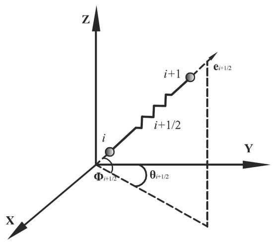
Figure 1.
Mooring model in global coordinate.
All forces along the mooring lines are assumed to be concentrated at the node.
Tension forces at the i-th node include the tension forces in the line segments on either side of the node i which are, respectively, indicated as Ti+1/2 and Ti−1/2.
where E is the elastic module; A is the cross-sectional area; li+1/2 is the original length of the segment between the i-th node and (i+1)-th node; li−1/2 is the original length of the segment between the i-th node and (i−1)-th node.
The tension force at node i is expressed as follows:
Wave forces on the mooring line are computed using the Morison equation, which assumes the force to be linearly summation of inertia and drag forces. The wave–particle velocity at node i is ui = [ux,i, uy,i, uz,i]T. The normal wave–particle velocity across the half of the upper segment that connects the i-th node is
Similarly, the normal wave–particle acceleration across the half of the upper segment that connects the i-th node is
The tangential wave particle velocity across the half of the upper segment that connects the i-th node is
and the corresponding acceleration across the half of the upper segment that connects the i-th node is
The inertia or drag forces are usually computed separately for directions normal and tangent to the lines. As the tangential component is usually small and can be neglected, it is assumed that the tangential inertia coefficient is zero. The inertia force on the upper and lower half segment on the side of node i is as follows:
where is the normal and tangential inertia coefficient.
Then, the inertia forces on node i including two lines segments on either side of the node are
where , and the normal inertia coefficient = 2.
The structural acceleration is not included in inertia forces, and it is usually accounted for by the inclusion of an added mass term in the mass matrix in the equation of motion.
where , and the normally added mass coefficient .
The added mass on node i is
Therefore, the mass, including added mass matrix, is
where represents the mass of two mooring line segments on each side of the i-th node.
Additionally, the force including weight and buoyancy is
where the buoyancy is denoted by , and is the density of seawater.
The drag force on the upper and lower half segment on the side of node i is calculated using Morrison’s equation. The tangential drag is assumed to be neglected as it is usually small.
where is the normal drag coefficient. is the normal relative velocity to the upper segment connected with node i, respectively.
where Vri is the relative velocity between the water–particle velocity from wave ui and current Vci at node i and the velocity of node .
The drag forces on the i-th node including two line segments on either side of the node are
where .
2.1. Dynamic Analysis in the Time Domain
The equation of motion is
where M is the mass matrix of mooring lines including added mass, and is the acceleration. The force consists of tension forces T, inertia force FI, drag force FD, weight, and buoyancy W.
The upper end connects with the vessel, and the bottom end is considered as a fixed point. The motion equation of mooring lines can be solved using numerical integration schemes. Here, the modified Euler method is applied. and are the known displacement and velocity of the mooring line, respectively, at time . The displacement and velocity of the line, and , at the time are evaluated as follows:
where is the time step. The new displacements, velocities, and accelerations of all the nodes can be evaluated easily according to this scheme.
It can be seen that the modified Euler method is very simple, and it can lead to accurate response evaluations. It is explicit and straightforward, which is different from the Newmark beta method, which needs iteration for each step. This method is conditionally stable, and the time step should satisfy the condition of stability as follows:
where T is the natural period of vibration of the line system.
2.2. Dynamic Analysis in the Frequency Domain
The dynamic analysis in the frequency domain is based on the linear system. There are nonlinear effects that can have an important influence on mooring line behavior. One is geometric nonlinearity, which is associated with large changes in the shape of the mooring line. The other is fluid loading, in which the Morrison equation is most frequently used to represent its effects on mooring lines. The drag force on the line is proportional to the square of the relative velocity between the water–particle velocity from the wave or current and the line’s velocity and hence is nonlinear. In addition, the contact of the line with the seabed is also nonlinear. These nonlinearities have to be linearized.
It is assumed that dynamic deflections around the static equilibrium position are small. The tangent stiffness matrix for the upper segment for node i is
The drag force can be linearized by the statistical linearization method. The nonlinear term in drag force is replaced by the linear form
where Ce is the equivalent linear coefficient, and Fm is a constant force vector. The normal water–particle velocity from wave is a Gaussian random process, the corresponding structure’s velocity , and the relative velocity is also a Gaussian random process. The Ce and Fm can be estimated from the minimization of the expected square error between the nonlinear and linearized forms. The expected square error is
Minimization of the error with respect to Ce and Fm leads to the following:
Since the relative velocity is normal to the centerline of the line, it has only two nonzero components in a coordinate system that has the tangent to the centerline as a basis vector. If the two components are uncorrelated, the evaluation of the expected values in the above equations can be simplified. We can choose the coordinate based on the principal directions of the relative velocity covariance matrix. One base vector of the coordinate system, denoted as axis 1, is in the direction of the maximum velocity variance and the other, denoted as axis 2, is in the direction of the minimum velocity variance. In this coordinate system, the two components of the relative velocity are uncorrelated, i.e., the covariance of vl and v2 is zero. Additionally, current velocity is in this coordinate system.
Therefore, the above equations can be rewritten as follows:
where is the probability density function of . Considering is a Gaussian random process and vl and v2 are uncorrelated, the probability density function is
The linearization needs the integration of double infinite integrals. Only a few special cases have the closed form of integration. For the one-dimensional drag force, the linearization results are
where .
If there is no current, then the linearization coefficient for one-dimensional drag force is
For the case in which the drag force is three dimensional, the integrals require numerical integration. The infinite integrals can be transformed into finite integrals by trigonometric functions, and the finite integrals are evaluated by trapezoidal rule [13]. Using the above linearization method, the linearized drag force at node i can be obtained as follows:
where is the orthogonal transformation from the local principal coordinate system to the global coordinate system.
where
After linearization, the equation of motion of mooring lines is transformed into the frequency domain in the form as follows:
Then, the right side of the equation of motion can be rewritten as G(ω)η(ω), where G(ω) is the force transfer function. the displacement responses can be obtained as
where H(ω) is the transfer function and H(ω) = (−ω2M + iωQ + K)−1G(ω).
Additionally, the velocity of lines is
The response spectral of displacement and top tension are
Mean square response of displacement and velocity are
Top tension can be obtained as
3. Numerical Case in the Time Domain
The codes for the dynamic analyses of mooring lines in the time domain were programmed using MATLAB. The numerical case analyses of single-component and multicomponent mooring lines were carried out. To verify this program, the results were compared with the results from commercial software, Orcaflex. The detailed properties of lines are listed in Table 1. The harmonic excitations were applied on the top end of the lines. The horizontal and vertical harmonic excitations represent the motions at wave frequency and low frequency of a floating structure, respectively.

Table 1.
Properties of the mooring line.
Three test cases were carried out and compared with the results from Orcaflex. The first case was a single-component mooring line only under harmonic excitation applied on its top end. There were no environmental loads and no seabed contact. In the second case, the environmental loads, wave, and current were applied to the line. The third case addressed multicomponent mooring lines. The lines were subjected to wave, current, and harmonic excitation. In addition, contact with seabed was also taken into account.
3.1. Single-Component Mooring Line under Harmonic Excitation
The dynamic response of a single-component mooring line, the R4 chain, was simulated. The mooring line was subjected to vertical, horizontal, and combined vertical and horizontal harmonic excitations, respectively. The given harmonic excitations are as follows:
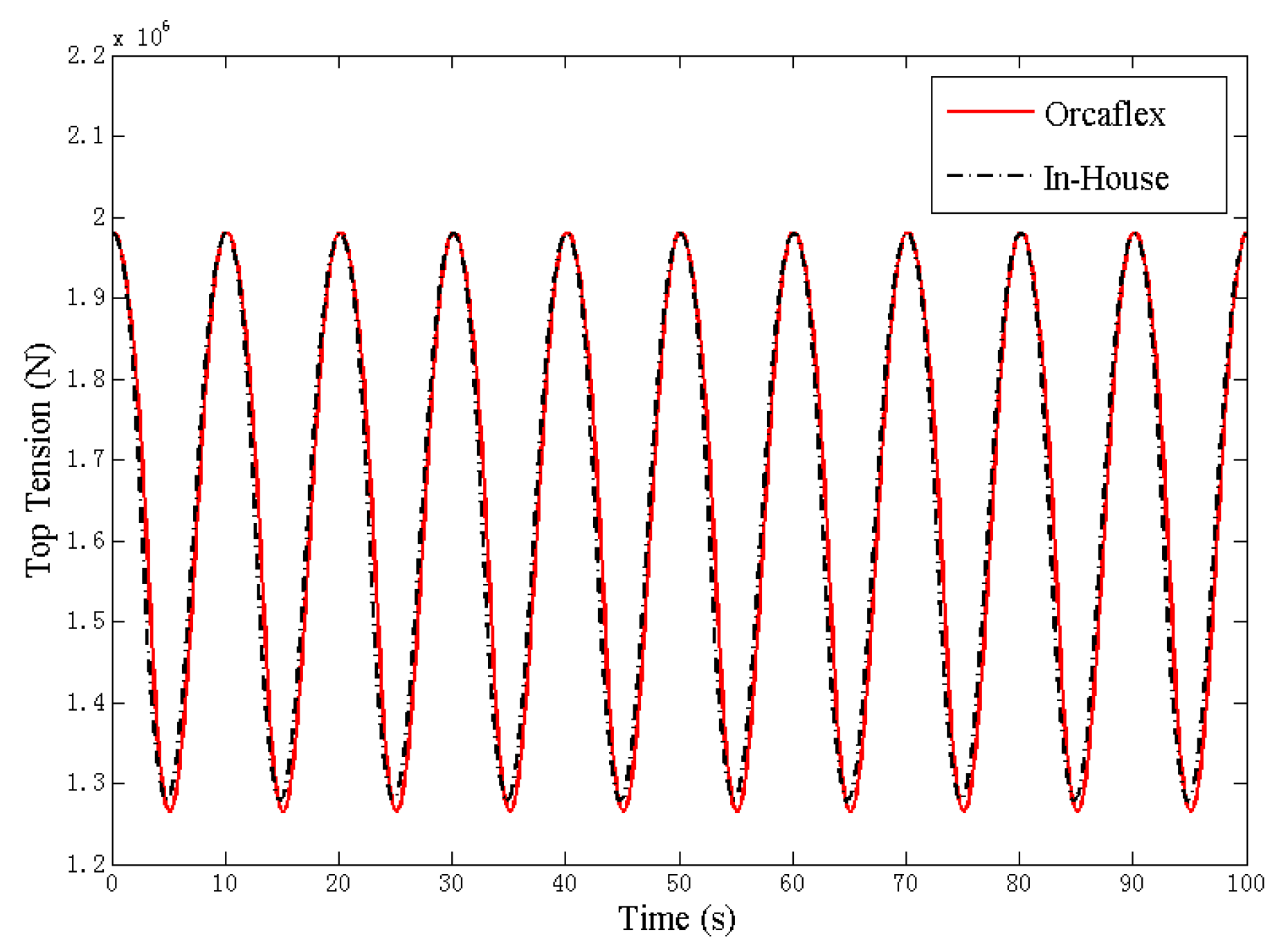
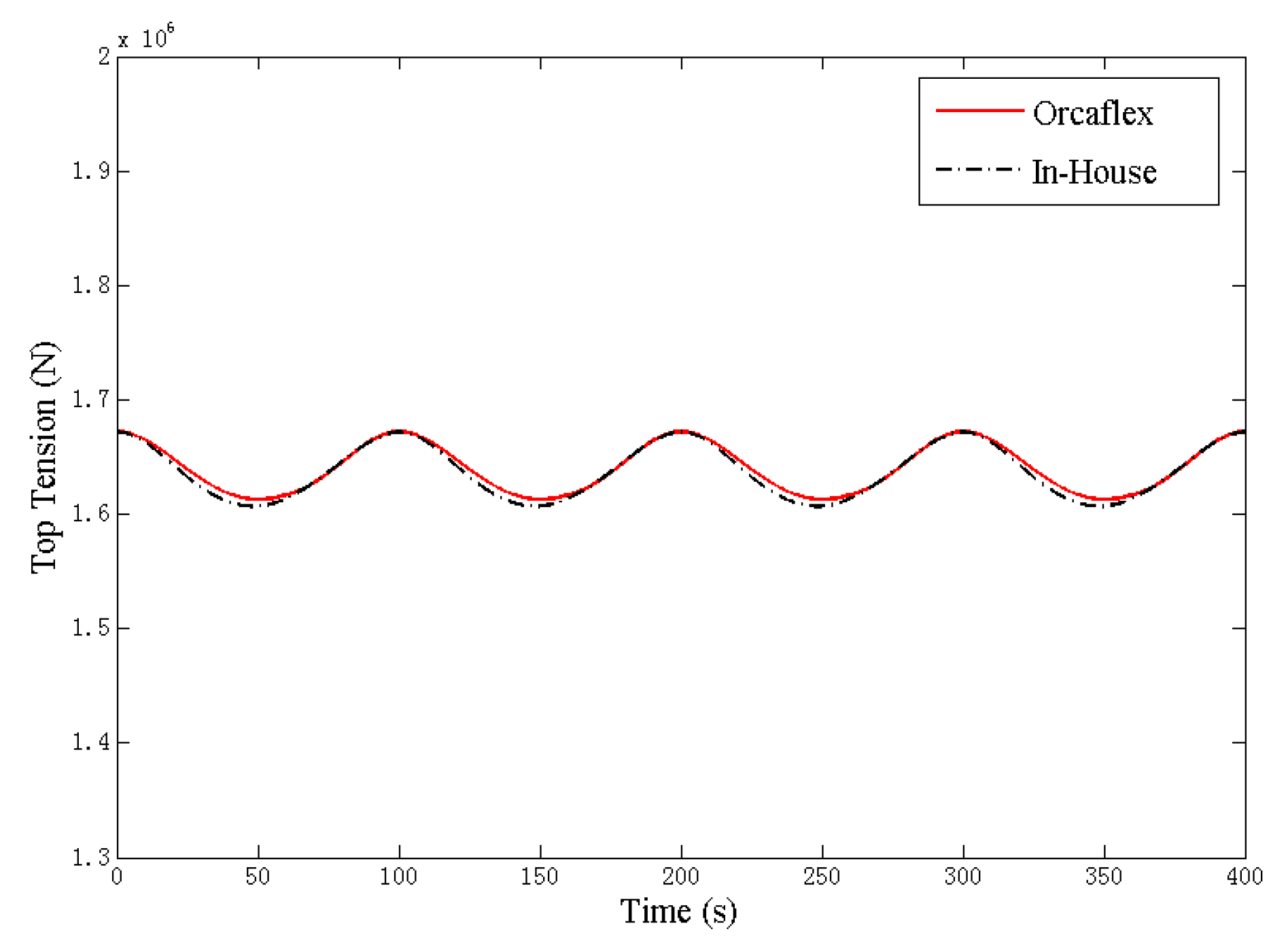
The environmental loads were not taken into account here. The water depth is 400 m. The length of the line is 400 m. The top end is 10 m under the water surface. The configuration of the mooring line is shown in Figure 2. Additionally, the results of dynamic analysis were compared with Orcaflex’s. There are 20 segments. Figure 3, Figure 4 and Figure 5 show the dynamic response of a single-component mooring line under vertical, horizontal, and combined vertical and horizontal harmonic excitations. According to the results, the codes agree well with the outputs of Orcaflex, and the top tension range is 1% greater in Orcaflex.
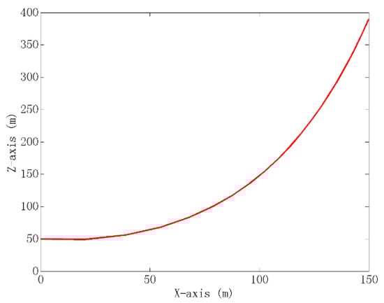
Figure 2.
Configuration of the single mooring line.

Figure 3.
Single mooring line under the vertical harmonic excitation.
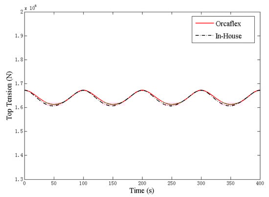
Figure 4.
Single mooring line under the horizontal harmonic excitation.
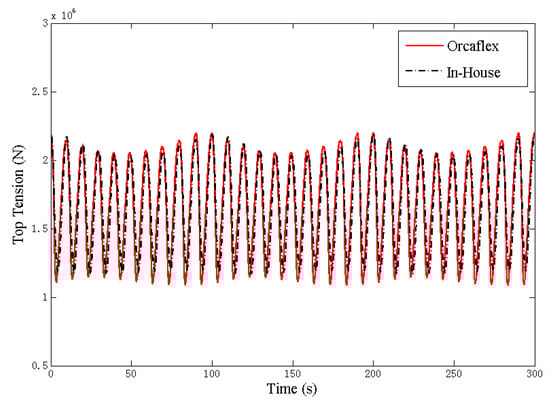
Figure 5.
Single mooring line under the combined vertical and horizontal harmonic excitations.
3.2. Single-Component Mooring Line under Harmonic Excitation with Wave and Current
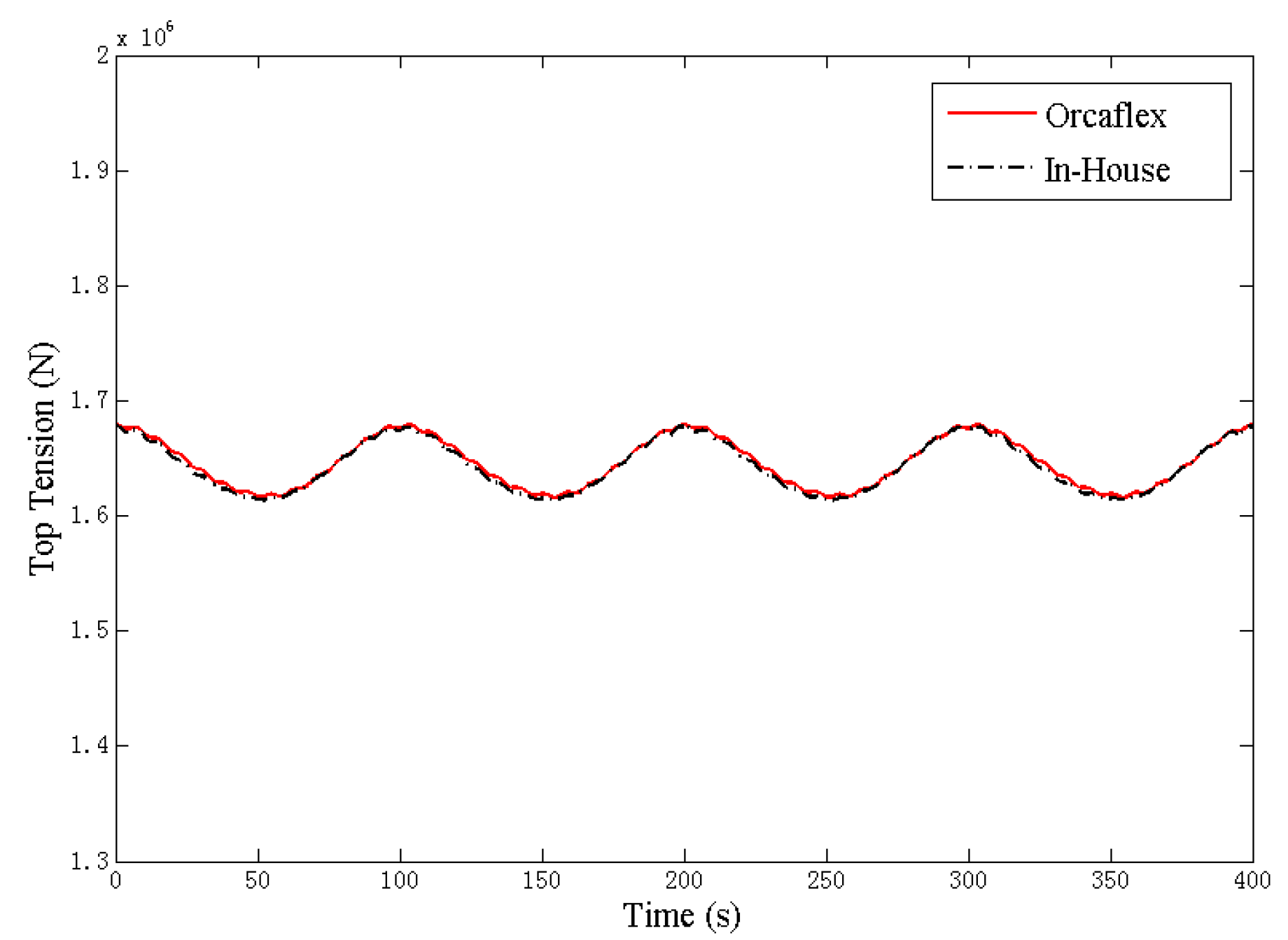
In this case, the environmental loads from wave and current were applied to the lines. The wave is an airy wave that has a wave height of 7.0 m and a period of 8.0 s. The current is 1 m/s in the x-direction and linear decay, along with the depth until zero at the seabed. Additionally, the mooring line was still subjected to three harmonic excitations, i.e., vertical, horizontal, and combined vertical and horizontal harmonic excitations. Both the results of mooring line dynamic analysis by the in-house code and Orcaflex are shown in Figure 6, Figure 7 and Figure 8. It can be seen that the agreement is well, and the difference is within 1%.
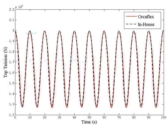
Figure 6.
Single mooring line under vertical harmonic excitation with wave and current.
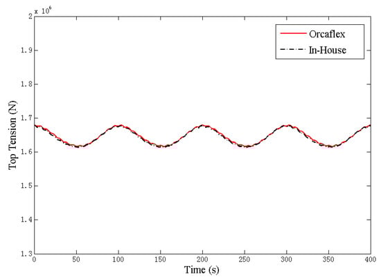
Figure 7.
Single mooring line under horizontal harmonic excitation with wave and current.
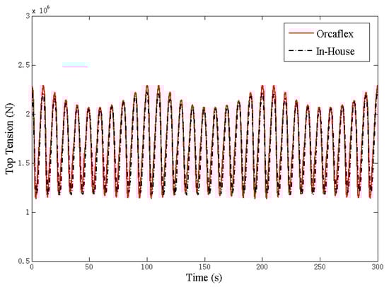
Figure 8.
Single mooring line under combined vertical and horizontal harmonic excitation with wave and current.
3.3. Multicomponent Mooring Line
This code can also carry out the dynamic analysis for multicomponent mooring lines. Here, a test case of a multicomponent mooring line (R4 chain-Spiral Strand wire-R4 chain) was simulated. The line length is 100, 400, and 1480 m, respectively. The configuration of the multicomponent mooring line is shown in Figure 9. The first part of the 100 m R4 chain was divided into five segments, and the second part of the spiral strand wire was divided into six segments. The third part of the R4 chain considered the seabed contraction, in which parts on the touch-down zone were meshed by 10 m per segment (in total 58 segments), and other parts, always on the seabed, were coarsely meshed by 100 m per segment. The given harmonic excitations are as follows:

Figure 9.
Configuration of the multicomponent mooring line.
Wave and current were the same as used in the single-component mooring line. In addition, seabed interaction was also considered. For the mooring line resting on the seabed, a modified bilinear spring is used to model the vertical contact force Fs on a node [14], which has the form in Equation (50). Friction effects are considered to be less significant for the system analyzed and are neglected. A gradual transition is proposed to account for numerical stability. The effects of wave and current are considered, using the same parameters in the single line case.
where a, b, c, and d is suitably chosen constants. In particular, d should be the value such that Fs is close to 0 when z is a suitable distance away from the seabed.
Dynamic response of multicomponent mooring line under vertical, horizontal, and combined vertical and horizontal harmonic excitations are shown in Figure 10, Figure 11 and Figure 12. According to the results of the dynamic analysis in the time domain, it can be seen that this program can perform as well as the commercial software, and the difference is within 3%.
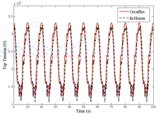
Figure 10.
Multicomponent mooring line under the vertical harmonic excitation.
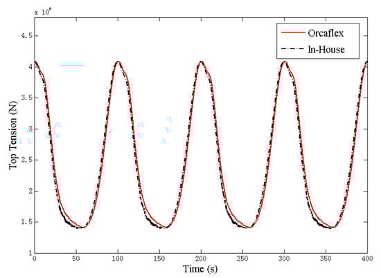
Figure 11.
Multicomponent mooring line under the horizontal harmonic excitation.
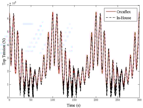
Figure 12.
Multicomponent mooring line under the combined vertical and horizontal harmonic excitation.
4. Numerical Case in the Frequency Domain
The code for the dynamic analysis of mooring lines in the frequency domain was programmed and compared with the results from Oraclex. Since Orcaflex cannot perform the dynamic analysis in the frequency domain, the dynamic responses in the time domain were transformed to responses in the frequency domain using FFT. The nonlinearities in the mooring lines were linearized using the aforementioned method. Additionally, cases of single-component and multicomponent lines were performed.
4.1. Mooring Line under Harmonic Excitation and Regular Wave
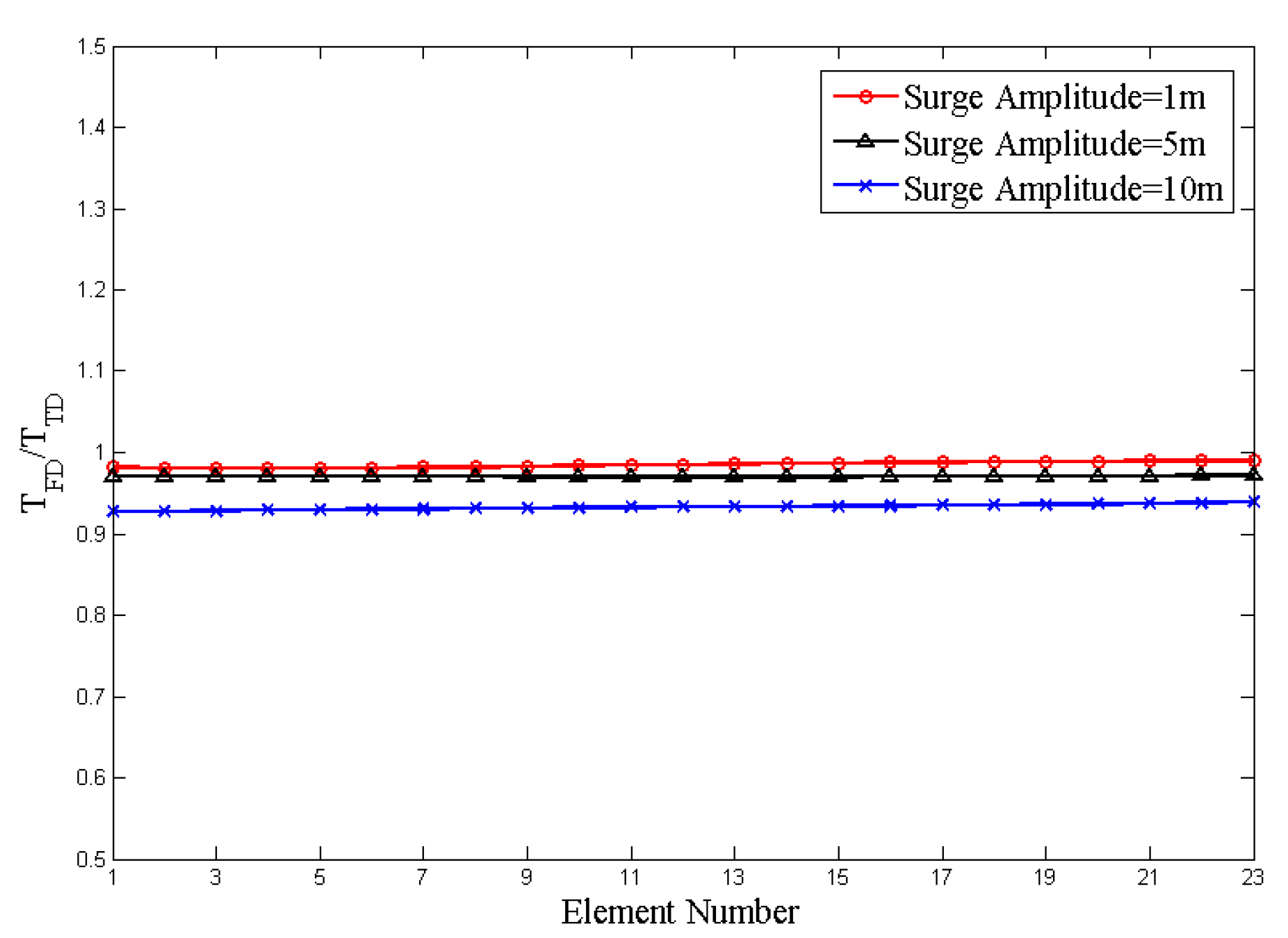
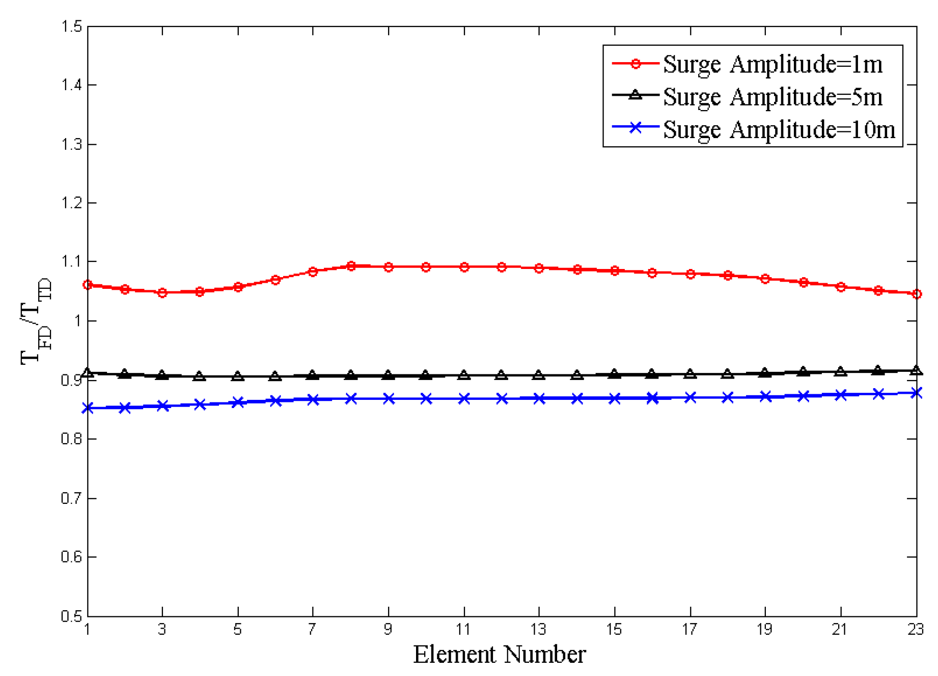
The dynamic analyses of a single-component mooring line, R4 chain, under different horizontal surge harmonic excitation were carried out in the frequency domain and time domain, respectively. The configuration of the mooring line is shown in Figure 2. The surge motion amplitudes of 1 m, 5 m, and 10 m with a period of 10 s were investigated. Figure 13 shows the ratio of dynamic tension amplitude in the frequency domain and time domain.

Figure 13.
The ratio of dynamic tension amplitude in the frequency domain and time domain under harmonic excitation.
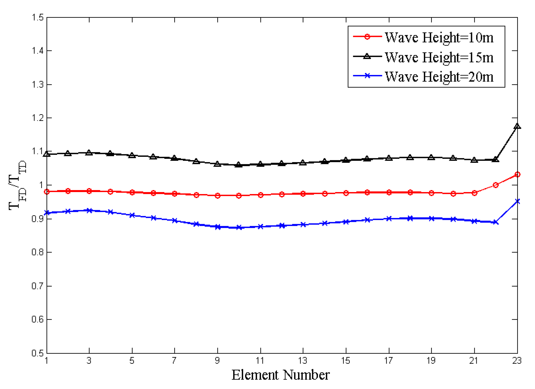
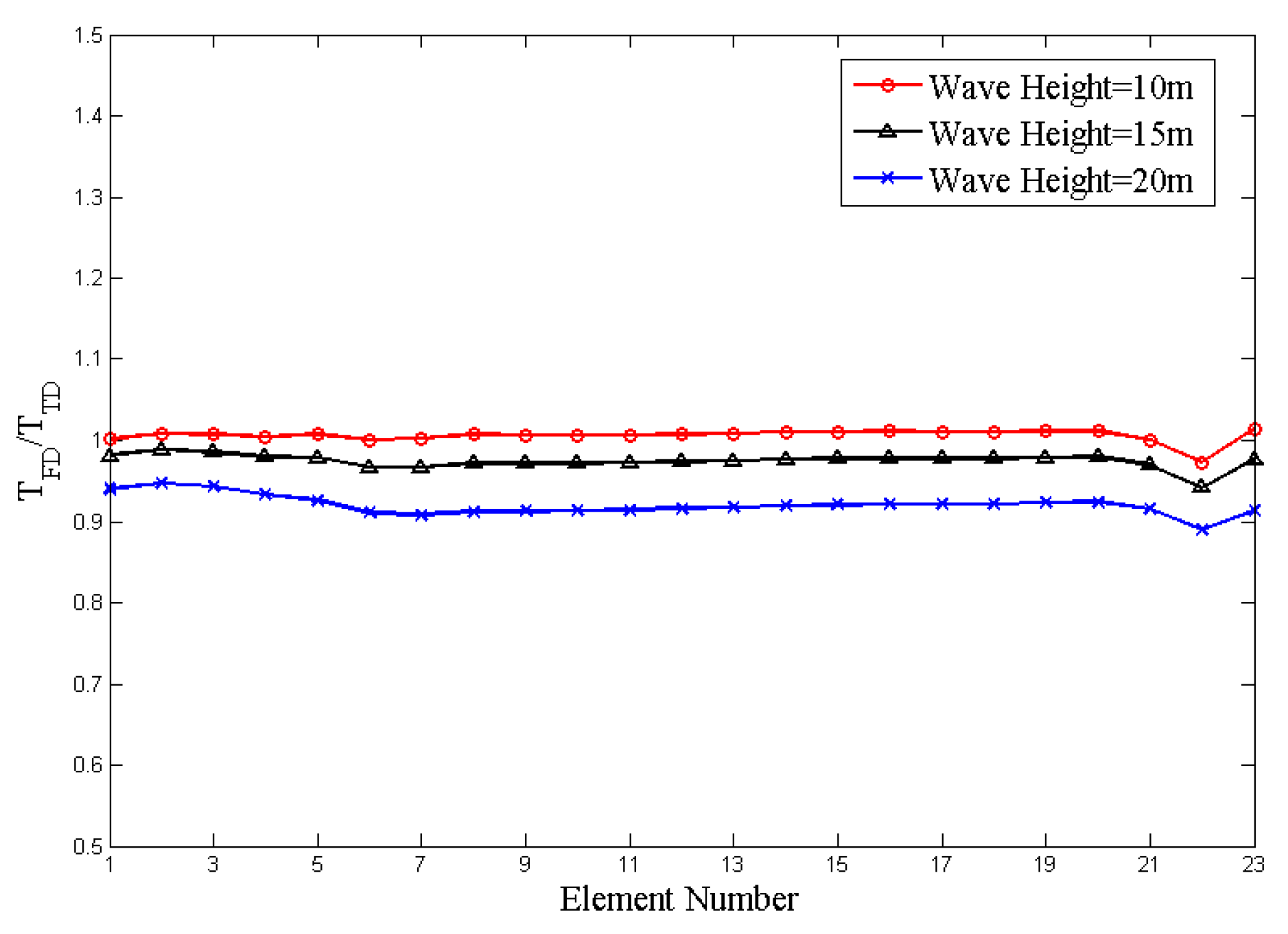
The frequency domain simulations of single-component mooring line under regular wave were carried out thereafter. The wave height is 10 m, 15 m, and 20 m, respectively. The ratios of dynamic tension amplitude in the frequency domain and time domain are shown in Figure 14.
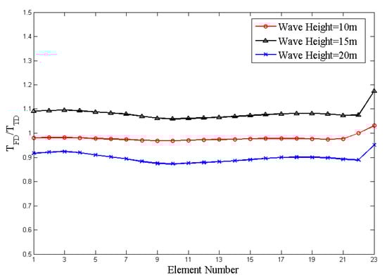
Figure 14.
The ratio of dynamic tension amplitude in the frequency domain and time domain under a regular wave.
The dynamic analyses of multicomponent mooring lines under different surge harmonic excitations were also carried out in the frequency domain and time domain, respectively. The configuration of the mooring line is shown in Figure 9. Figure 15 shows the ratio of dynamic tension amplitude in the frequency domain and time domain with the surge motion amplitudes of 1 m, 5 m, and 10 m. The ratios of dynamic tension amplitude in the frequency domain and time domain under wave height of 10 m, 15 m, and 20 m are shown in Figure 16.
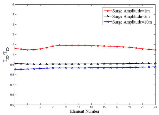
Figure 15.
The ratio of dynamic tension amplitude in the frequency domain and time domain under harmonic excitation.

Figure 16.
The ratio of dynamic tension amplitude in the frequency domain and time domain under a regular wave.
4.2. Single-Component Mooring Line under Random Wave with Current
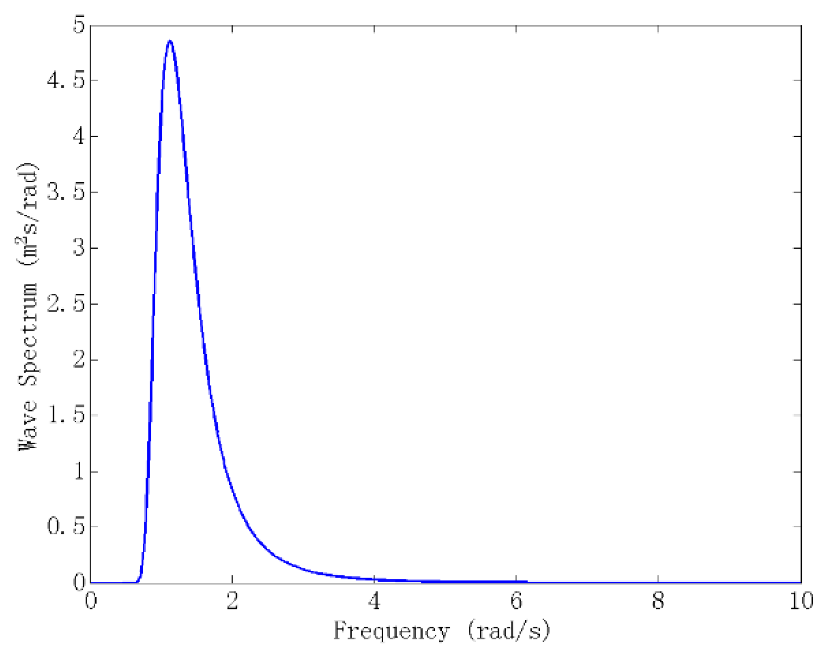
The dynamic analysis of a single-component mooring line, R4 chain, was simulated under a random wave. The random wave is defined by the ISSC spectrum as follows. The significant wave height is 7.8 m, the peak period is 5.6 s, and the spectrum is shown in Figure 17.
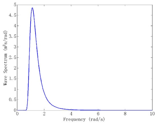
Figure 17.
Wave spectrum.
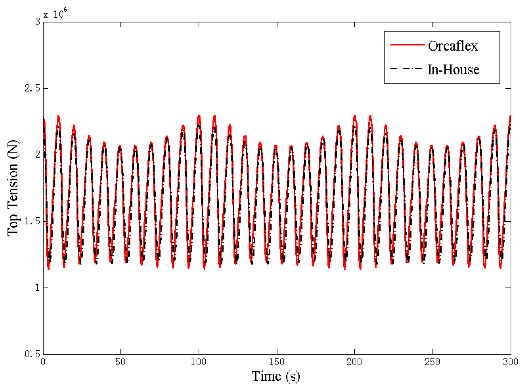
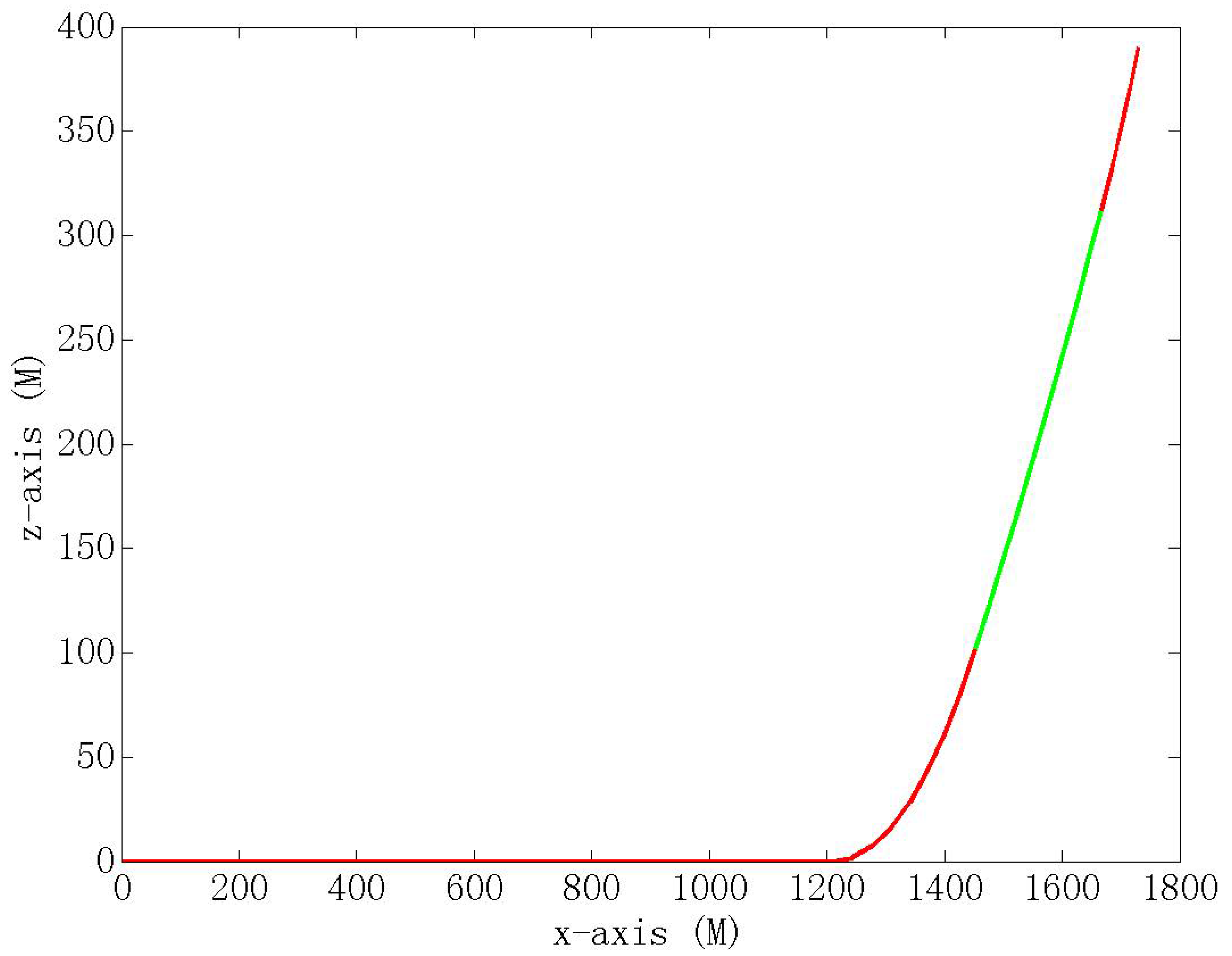
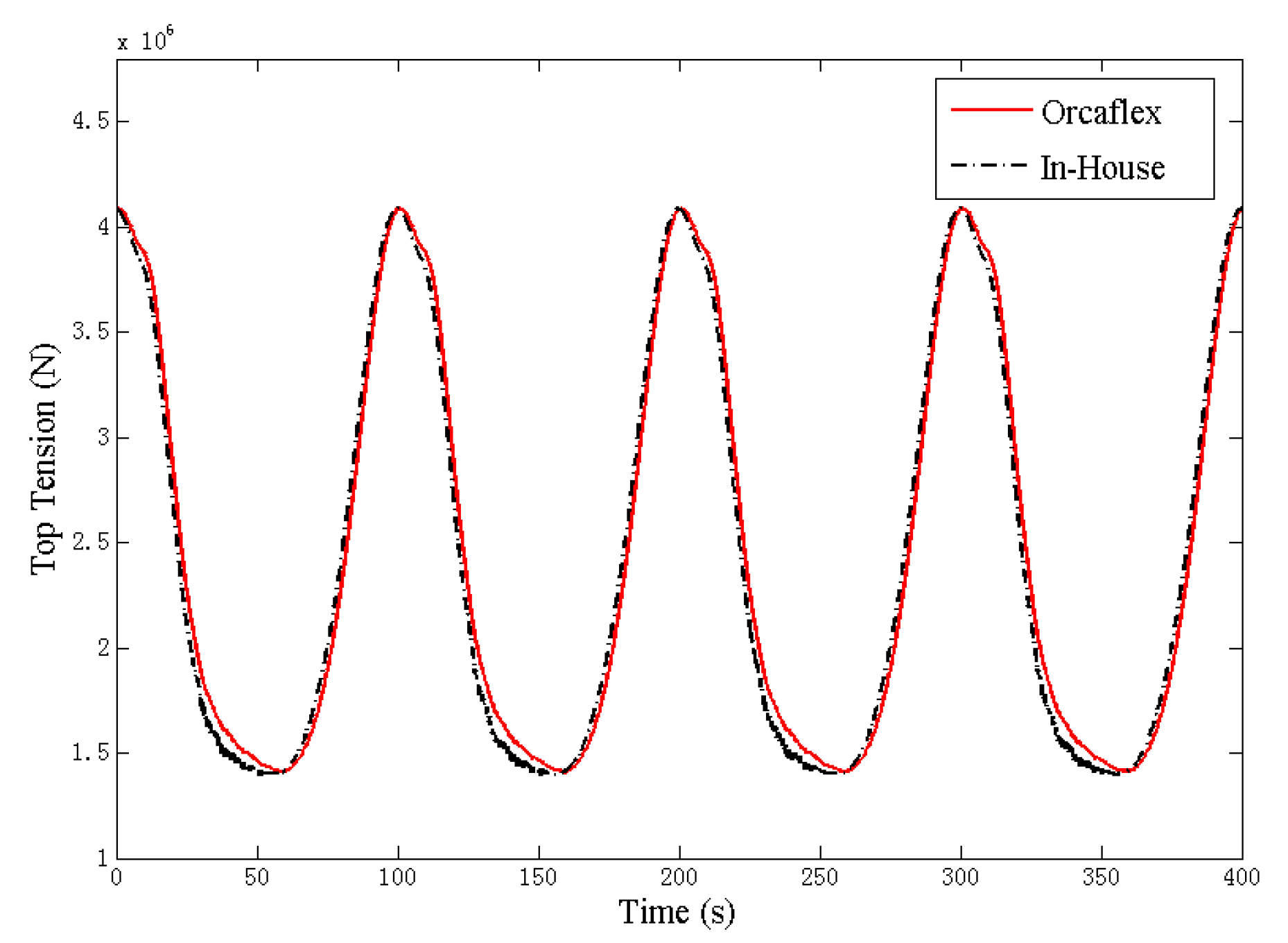
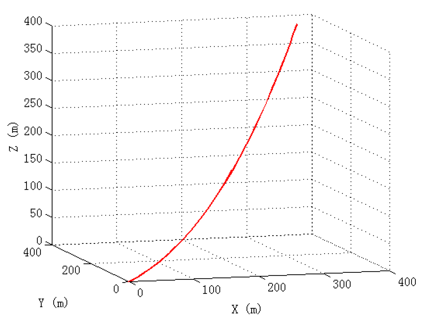
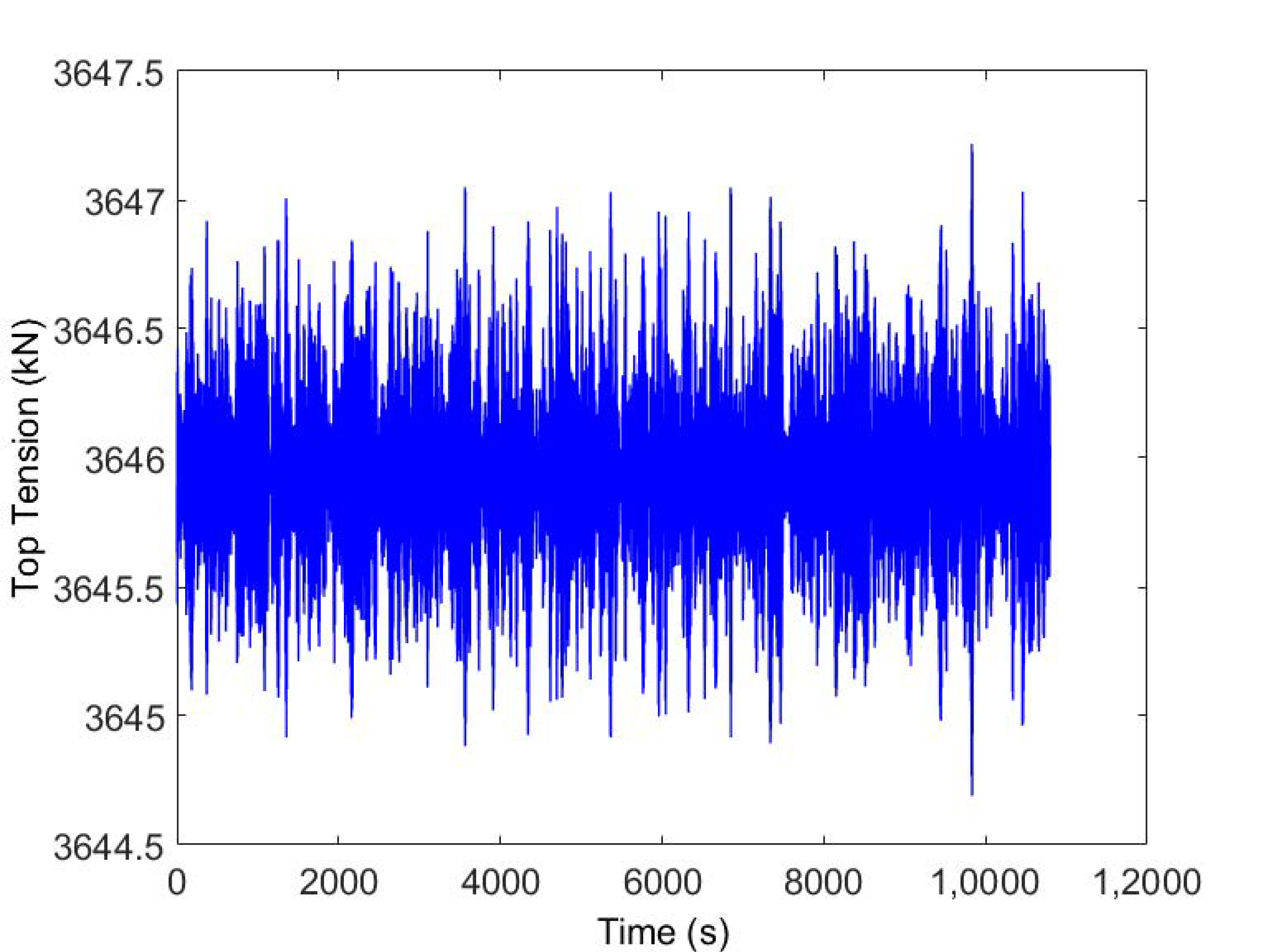
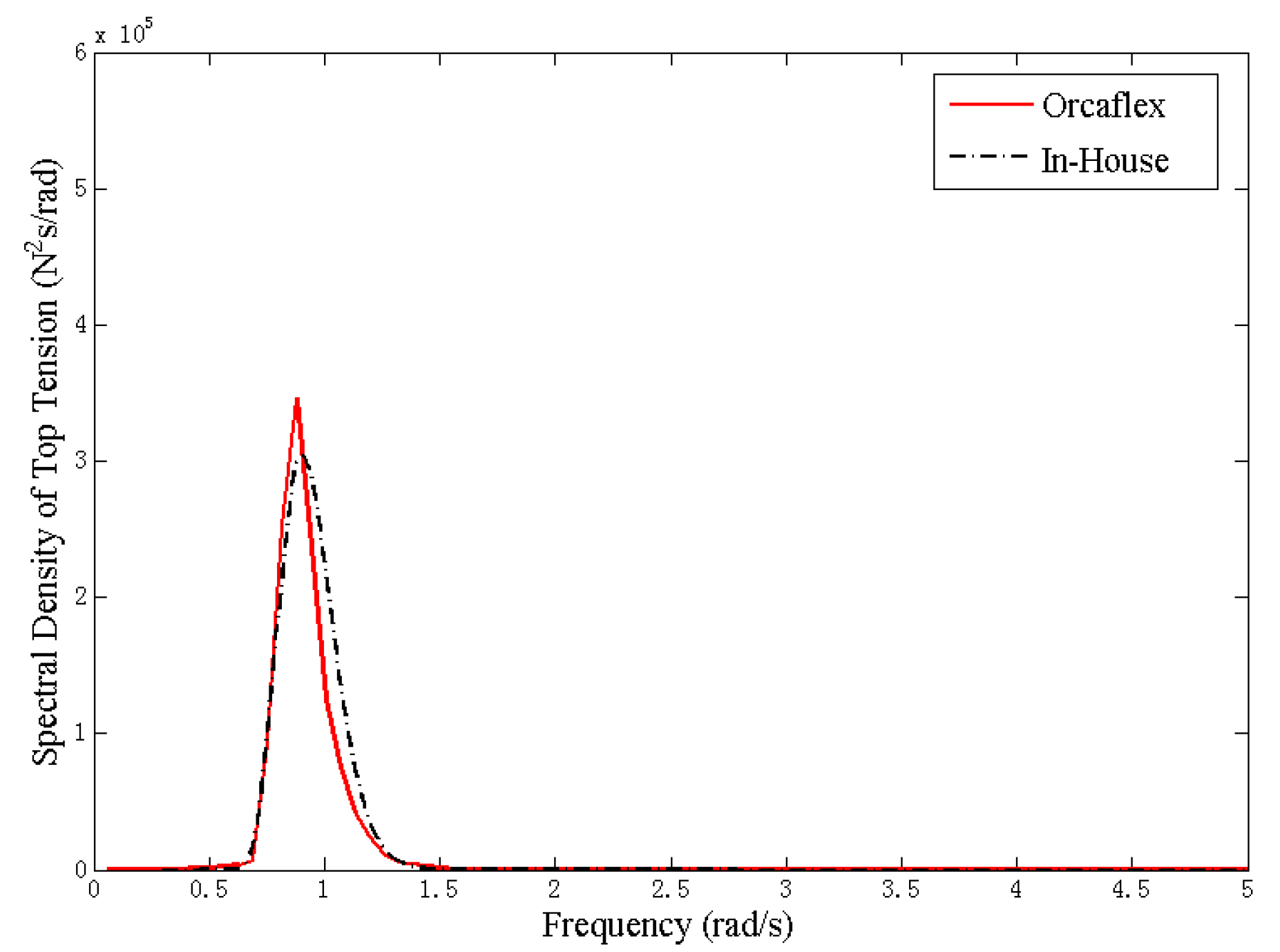
The current velocity is 1 m/s in the x-direction. The configuration of the mooring line is shown in Figure 18. The length is 668.8 m, and the water depth is 400 m. Both top and bottom are pinned, the top is at (366.89, 366.89, 390) and the bottom is at the origin point. After linearization and the frequency analysis, the spectral density of top tension is presented in Figure 19. The dynamic analysis in the time domain is simulated for 3 h using Orcaflex, as shown in Figure 20, and then transformed the response to the frequency domain. The standard deviation of top tension is shown in Table 2. The difference is 13.41%.

Figure 18.
Configuration of the single mooring line.
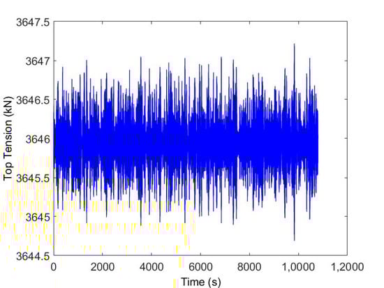
Figure 19.
Spectral density of top tension single mooring line.
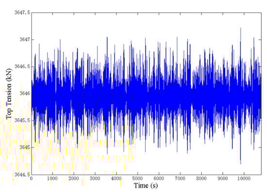
Figure 20.
Top tension in time series (3 h) of single-component line.
Table 2.
The standard deviation of top tension for single-component case.
4.3. Multicomponent Mooring Line under Random Wave with Current
The frequency analysis for a multicomponent (R4 chain-Spiral Strand wire-R4 chain) mooring line was also carried out under the random waves. The line configuration is shown in Figure 21. The length is 100 m, 300 m, and 268.8 m, respectively. Both ends were pinned, and positions were the same as the single-component line.
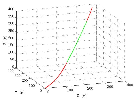
Figure 21.
Configuration of the multicomponent mooring line.
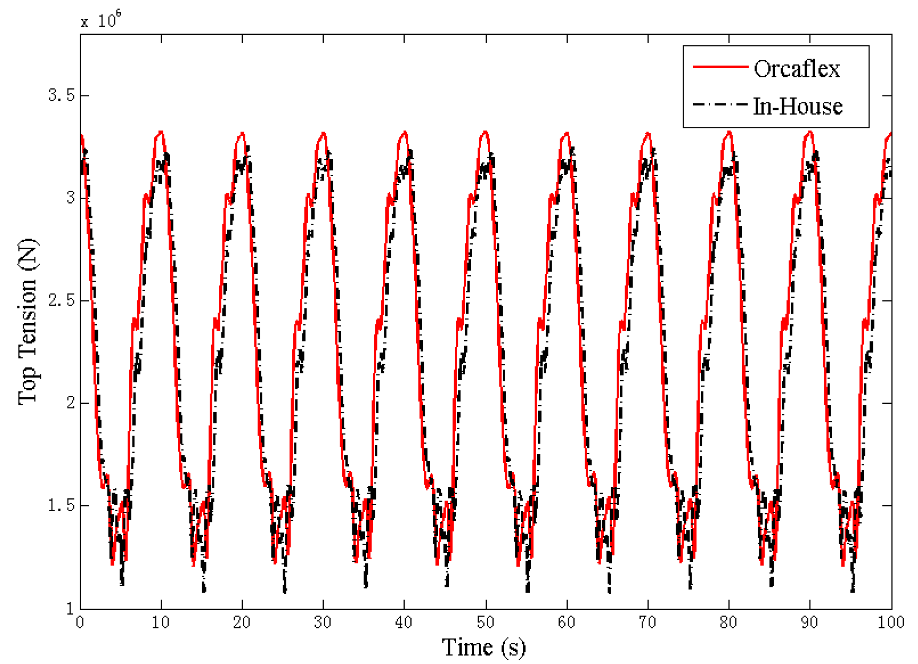
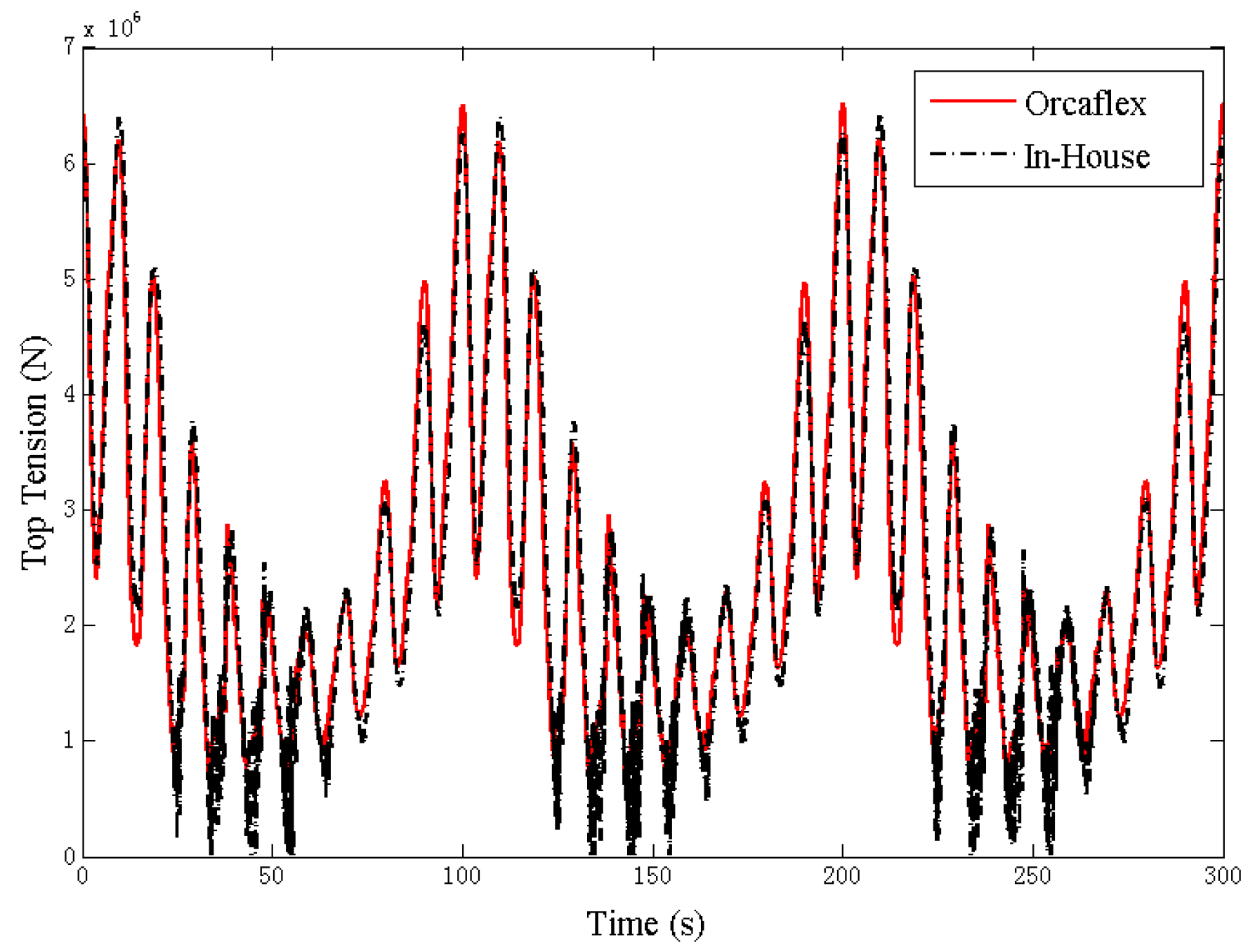
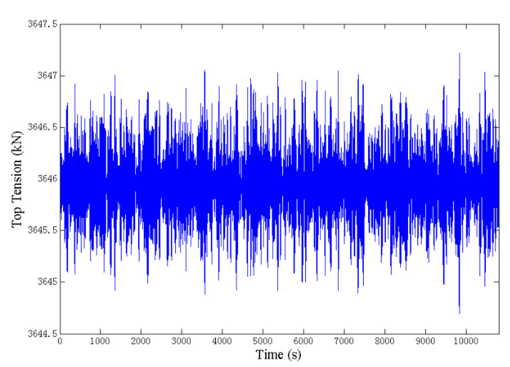
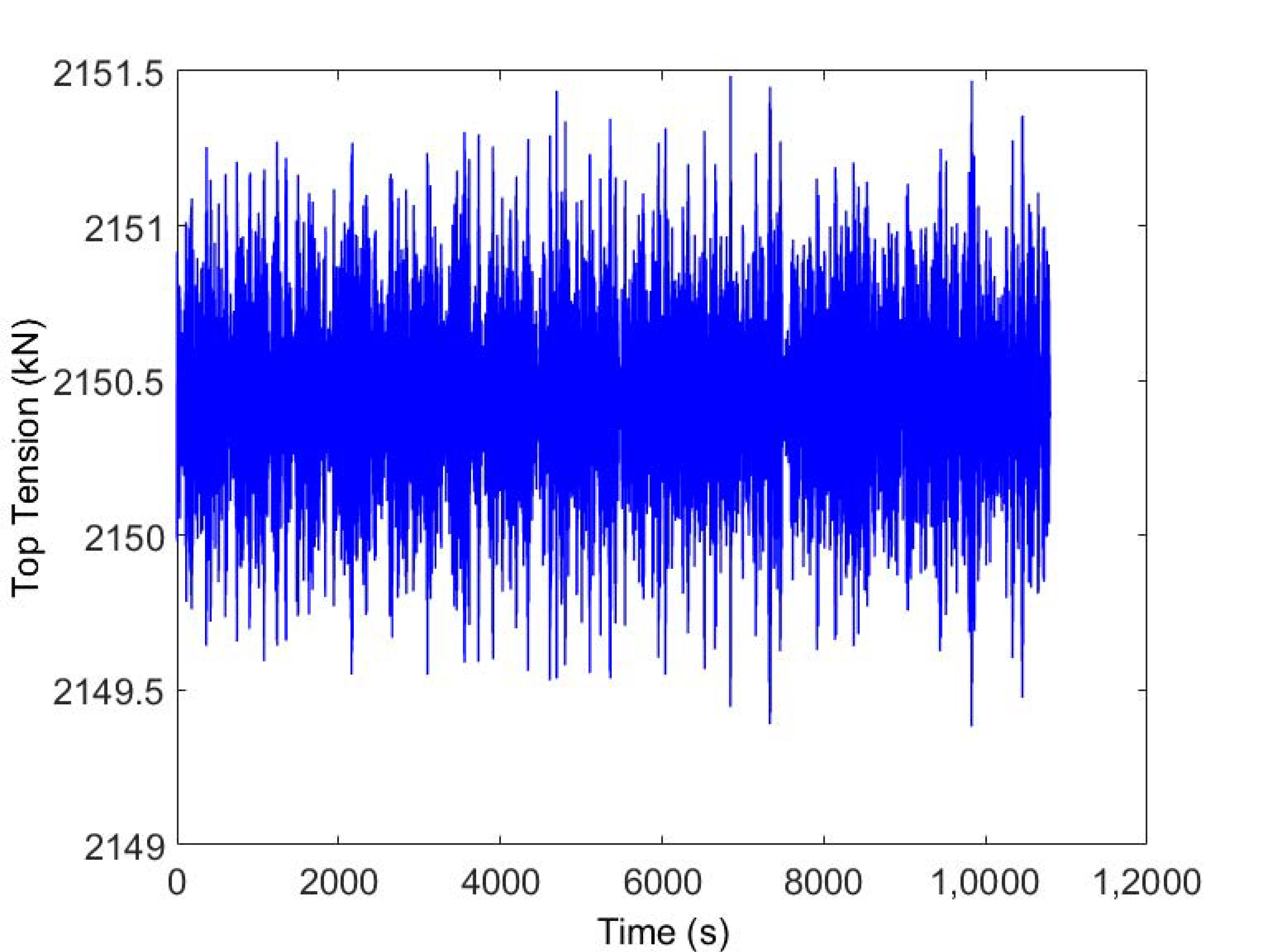
The dynamic analysis in the time domain was also simulated for 3 h using Orcaflex, as shown in Figure 22. Additionally, the response of top tension in time series was transformed to the frequency domain. The frequency analysis for the multicomponent line was carried out to obtain the spectral density of top tension, which is presented in Figure 23. The standard deviation of top tension is shown in Table 3. The difference between them is 6.16%.
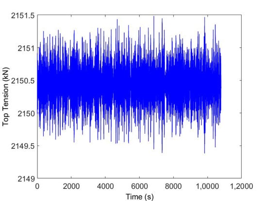
Figure 22.
Top tension in time series (3 h) of multicomponent line.
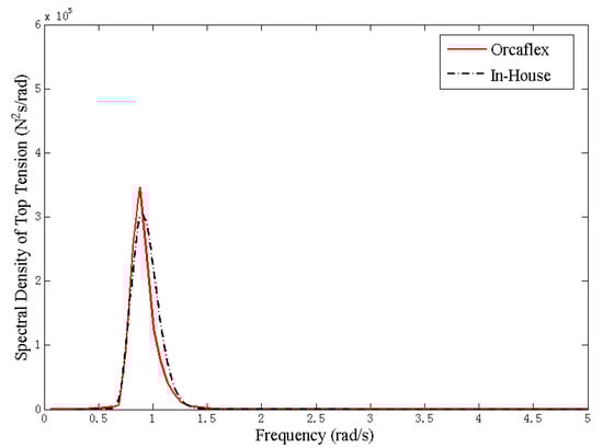
Figure 23.
Spectral density of top tension multicomponent line.
Table 3.
The standard deviation of top tension for the multicomponent case.
5. Conclusions
This paper developed a numerical scheme for dynamic analysis of mooring lines in the time domain and frequency domain based on the lumped mass method. The modified Euler method, a direct and simply explicit algorithm, was employed to carry out the dynamic analysis of mooring lines in the time domain. The mooring lines under horizontal, vertical, and combined harmonic excitations were studied. The studied cases included single-component and multicomponent mooring lines, and the seabed contact was also taken into account. An improved frame invariant stochastic linearization method was applied to the nonlinear hydrodynamic drag term for the frequency domain dynamic analysis. The cases of single-component and multicomponent mooring lines were studied. The codes were validated by comparison with commercial software, Orcaflex. The comparison of results showed that time and frequency domain results agree well with nonlinear time domain results.
Author Contributions
Conceptualization, S.H. and A.W.; methodology, A.W.; software, A.W.; validation, A.W.; formal analysis, A.W.; investigation, S.H.; resources, A.W.; data curation, A.W.; writing—original draft preparation, A.W.; writing—review and editing, S.H. and A.W.; project administration, S.H.; funding acquisition, S.H. Both authors have read and agreed to the published version of the manuscript.
Funding
This research was funded by the National Natural Science Foundation of China, Grant Number 51979157.
Institutional Review Board Statement
Not applicable.
Informed Consent Statement
Not applicable.
Data Availability Statement
Not applicable.
Conflicts of Interest
The authors declare no conflict of interest.
References
- Low, Y.M.; Langley, R.S. Dynamic analysis of a flexible hanging riser in the time and frequency domain. In Proceedings of the International Conference on Offshore Mechanics and Arctic Engineering, Hamburg, Germany, 4–9 June 2006; Volume 4, pp. 161–170. [Google Scholar] [CrossRef]
- Huang, S. Dynamic analysis of three-dimensional marine cables. Ocean. Eng. 1994, 21, 587–605. [Google Scholar] [CrossRef]
- Nakajima, T.; Motora, S.; Fujino, M. On the dynamic analysis of multi-component mooring lines. In Proceedings of the Offshore Technology Conference, Houston, TX, USA, 3–6 May 1982. [Google Scholar]
- Huang, S.; Vassalos, D. A numerical method for predicting snap loading of marine cables. Appl. Ocean. Res. 1993, 15, 235–242. [Google Scholar] [CrossRef]
- Hahn, G.D. A modified Euler method for dynamic analysis. Int. J. Numer. Methods Eng. 1991, 32, 943–955. [Google Scholar] [CrossRef]
- Chakrabarti, S.K.; Cotter, D.C. Motion analysis of articulated tower. J. Waterw. Port. Coast. Ocean. Div. 1979, 105, 281–292. [Google Scholar] [CrossRef]
- Atalik, T.S.; Utku, S. Stochastic linearization of multi-degree-of-freedom non-linear systems. Earthq. Eng. Struct. Dyn. 1976, 4, 411–420. [Google Scholar] [CrossRef]
- Krolikowski, L.P.; Gay, T.A. An improved linearization technique for frequency domain riser analysis. In Proceedings of the 12th Offshore Technology Conference, Houston, TX, USA, 5–8 May 1980. [Google Scholar]
- Spanos, P.D.; Ghosh, R.; Finn, L.D.; Halkyard, J. Coupled analysis of a spar structure: Monte Carlo and statistical linearization solutions. J. Offshore Mech. Arct. Eng. 2005, 127, 11–16. [Google Scholar] [CrossRef]
- Wu, S.C. The effects of current on dynamic response of offshore platforms. In Proceedings of the Offshore Technology Conference, Houston, TX, USA, 2–5 May 1976. [Google Scholar]
- Hamilton, J. Three-dimensional Fourier analysis of drag force for compliant offshore structures. Appl. Ocean. Res. 1980, 2, 147–153. [Google Scholar] [CrossRef]
- Langley, R. The linearisation of three dimensional drag force in random seas with current. Appl. Ocean. Res. 1984, 6, 126–131. [Google Scholar] [CrossRef]
- Rodenbusch, G.; Garrett, D.L.; Anderson, S.L. Statistical linearization of velocity-squared drag forces. In Proceedings of the 5th International Offshore Mechanics and Arctic Engineering (OMAE) Symposium, Tokyo, Japan, 13 April 1986. [Google Scholar]
- Ghadimi, R. A simple and efficient algorithm for the static and dynamic analysis of flexible marine risers. Comput. Struct. 1988, 29, 541–555. [Google Scholar] [CrossRef]


Publisher’s Note: MDPI stays neutral with regard to jurisdictional claims in published maps and institutional affiliations. |
© 2021 by the authors. Licensee MDPI, Basel, Switzerland. This article is an open access article distributed under the terms and conditions of the Creative Commons Attribution (CC BY) license (https://creativecommons.org/licenses/by/4.0/).