Influence of Sand Trapping Fences on Dune Toe Growth and Its Relation with Potential Aeolian Sediment Transport

Abstract

This study provides insights into dune toe growth around and between individual brushwood lines of sand trapping fences at the dune toe of coastal dunes using digital elevation models obtained from repeated unmanned aerial vehicle surveys. Prevailing boundary conditions, especially sediment supply, as well as the porosity and arrangement of the installed sand trapping fences significantly influence the effectiveness of different configurations of sand trapping fences. The dune toe growth is significant immediately after constructing a new sand trapping fence and decreases over time. According to the results presented in this study, for sand trapping fences that have been in place longer, the protruding branch height and the porosity of the remaining branches play a minor role in trapping sand. Sand trapping fences with lower permeability favour localized coastal dune toe growth directly at their brushwood lines, whereas fences with higher porosity allow for more sediment deposition further downwind. The trend in dune toe changes can be roughly predicted by integrating potential sediment transport rates calculated with hourly meteorological data.

1. Introduction

Coastal dunes are a natural barrier against storm surges and act as a sediment resource in case of erosive storm events, thereby offering protection for the low-lying hinterland against flooding and sea-level rise [1,2,3,4]. Furthermore, they have a natural protective function within the framework of nature conservation and serve for recreation [5]. However, the coastal dune system, in particular the foredune, is complex and highly dynamic as natural processes drive the dune development [5,6]. Long-term coastal dune development results from the sum of erosive processes due to hydrodynamic forces during storm surges and accretive processes due to aeolian sediment transport processes, resulting in growing or eroding coastal dunes [4,7,8]. Additionally, coastal management interventions like beach nourishments, installing sand trapping fences, the presence of vegetation, the sediment grain size, or the beach width can, amongst others, influence the development of the coastal dunes [4,6,9,10,11,12,13].

To support the restoration and maintenance of beach and dune systems, accurate knowledge of beach-dune interaction and the effectiveness of coastal protection measures to strengthen coastal dunes is required [5,14,15]. Generally, a good empirical understanding of dune erosion and wave-dune interaction processes exists and has been extensively studied [8,16,17,18]; however, the prediction of dune growth is a significant challenge due to the complexity of influencing factors, e.g., coastal dune formation, aeolian sediment transport, vegetation, or sediment moisture. These factors and their interaction make the understanding of the morphological and volumetric changes of the dune system a major challenge when utilizing building with nature methods for designing coastal protection measures [6,19,20]. The literature on aeolian sediment transport can, e.g., be found in Bagnold (1941) [21], van Rijn And Strypsteen (2019) [7], Baas And Sherman (2006) [20] or Sherman et al. (2012) [22].

Where a positive sediment supply exists, sand trapping fences as a widely used nature-based solution can often be found along the coastline of barrier islands at the seaward dune slope close to the dune toe. They are part of the coastal protection measures [2,23].

Generally, fences control air and water flow, sediments, and direct people flow or animals [24]. Depending on their purpose, they can be differentiated into two different types: wind fences and sand-trapping fences [24,25,26]. Wind fences are mainly used in arid and desert regions and aim to reduce wind velocity, prevent wind-induced erosion, and, e.g., protect transport infrastructure or monetary assets against heavy wind or sediment loads [26,27,28,29]. On the other hand, in coastal regions, sand trapping fences are placed with the following purposes: rehabilitating eroded areas from storm surges or blowouts in the coastal dunes, for reinforcement of the coastal dune toe, for protecting transport infrastructure or monetary assets from drifting sand, to control human access to nature reserve, and to initiate the formation of coastal dunes by supporting the selective deposition of sand [30,31]. While wind velocity reduction has already been extensively studied for wind fences [27,30,32,33], only a few detailed studies, e.g., [23,24,25,31,34,35,36,37], about sand trapping fences for initiating and facilitating the establishment of the dune toe are available. There is currently a research demand on sand-trapping fences in coastal areas for the position relative to the beach profile, the porosity and height of the fence, and the arrangement of the fence [25,36].

In this work, sand trapping fences with the primary aim to strengthen the dune toe are considered. Figure 1a shows an aerial photograph of the sand trapping fence on Norderney with brushwood lines parallel and orthogonal to the coastal dunes and Figure 1b a close-up of the sand trapping fence from the viewpoint of the coastal dunes showing sand being trapped in between the brushwood lines.

The individual brushwood lines generally reduce the wind velocity, so that sediment can accumulate at the individual brushwood lines. These processes initiate and facilitate the dune toe development [38].

Currently, the design of these sand trapping fences on the East Frisian islands, i.e., the arrangement of the brushwood lines parallel and orthogonal to the coastal dunes, the position of the brushwood lines relative to the dune profile as well as the porosity and the height of the sand trapping fences is based on empirical knowledge, creating further uncertainties for implementing these coastal protection measures [36].

This study presents insights into the effectiveness of different sand trapping fence configurations to contribute to the formation of the dune toe. Thus, the results will help to improve and adapt methods for nature-based solutions of foredune restoration in coastal areas.

Therefore, during field campaigns from May 2020 until March 2021, we monitored the terrain elevation heights of two different study sites to gain more insight into the dune toe development influenced by different configurations of a sand trapping fence. As a result, the following research goals are set:

(1)

Determination of the porosity of the different sand trapping configurations.

(2)

Description of the temporal changes of dune toe volume and dune profiles at the sand trapping fence under consideration of the prevailing boundary conditions.

(3)

Evaluation of the different sand trapping fence configurations to trap sand effectively.

(4)

Investigation on the relation between dune toe volume changes and potential aeolian sediment transport.

First, the regional settings, the coastal protection measures, and the study sites are described in detail. After describing the applied methodology, the results are presented and discussed. Finally, the manuscript concludes with a discussion and an outlook.

2. Regional Setting and Coastal Protection Measures

The East Frisian Islands, see Figure 2, form a natural barrier island system in the German North Sea. The development and the shape of these sandy natural barrier islands are continuously changing as part of a highly dynamic morphological system due to the sea level rise, varying sediment availability, sandbar relocations, and storm surges [39,40]. For a detailed study on beach-dune systems near tidal inlets the readers are referred to Silva (2019) [13].

The whole barrier island system stretches over ~90 km. Six main tidal inlets dissect the islands, see Figure 2a [2,41]. Between this island system and the mainland (distance ~3–20 km) extensive areas with tidal flats exist.

The East Frisian Islands are influenced by tidal energy as well as wave energy and can be categorized as mesotidal barrier islands with semi-diurnal tides and a tidal range of around T_R ~2.5 m (Norderney, Riffgat) up to T_R ~2.7 m (Langeoog, port entrance) [43,44,45]. As the tide rises, the tidal basins are filled, and they are emptied again as the tide falls [46]. Incoming waves generally run in from the directions between northwest and southwest; only the northwest components of waves are incident on the study site [47].

Figure 3a shows the hourly averaged wind data at the weather station Norderney at the height of 11 m above the ground and (b) Spiekeroog (see Figure 3b) at the height of 14 m above the ground. The wind data from 1 May 2020 to 31 March 2021 are depicted as a wind rose. Over the measured time period, a significant southwest component of the wind with magnitude wind velocities of up to ~20 m/s and mainly oblique offshore wind conditions concerning the coastline were recorded. The oblique onshore wind occurred less frequently but, on average, reached higher wind velocities [48]. The strong southwesterly wind conditions have little effect on the local water level at both study sites, whereas the less frequent but strong northwesterly wind has a longer fetch length and can lead to higher water levels locally.

Both weather stations provide similar results, with Spiekeroog always tending to measure higher magnitude wind velocities than Norderney. This is because the nearby urban area attenuates wind velocities from Norderney’s weather station.

The East Frisian island Langeoog (see Figure 2b) covers ~20 km², and its morphology generally consists of a natural sandy beach followed by foredunes and older dune landscapes. The fully established foredune is ~ 20 m high and partially covered with the European Marram grass (Ammophila arenaria) [2,36]. The island has a coastal dike line of 5.5 km (red line) in the southwest and a coastal dike line (red line) of 0.3 km in the south, while coastal dunes (orange areas) over ~20.3 km protect the coastline from the southwest side of the island northward towards the east. A little part of the coastline is additionally protected by dike revetments (red double line) in the west. In the northwest of the island, sand nourishments are carried out if required (yellow dotted line). The study site Langeoog is located north of the island at the dune toe, see Figure 2b. The beach comprises quartz sand with a median grain size of d₅₀ = 218 µm [36]. The beach has a relatively steep slope with m ~ 1:50. The beach width W [m], indicated as the distance between a defined water level (average of the high tide level MHW or average of the low tide level MNW) and the dune toe level (z = +3 mNHN [49,50]), varied from ~300 m during MNW = −1.3 mNHN [43] to ~70 m during MHW = +1.4 mNHN [43]. When the sand trapping fences were investigated in this study, the dry beach width was always W > 50 m. In July 2020, beach nourishments with a sand volume of V = 700.000 m³ at Pirolatal on Langeoog island, 1.5 km west of the study site, were conducted.

With an area of ~26 km², Norderney (see Figure 2 ©) is the second-largest East Frisian island. It has coastal dunes (orange areas) stretching over ~12.1 km from the southwestern side of the island northward towards the isl’nd’s center with heights up to 20 m. The coastal dunes are also in part covered with Ammophila arenaria. The beach slope m ~ 1:200 is much lower on Norderney than on Langeoog. The coastline is over ~10 km protected by coastal dikes (red line) in the south. Additionally, the dike line is partly protected by revetments (red double line) and massive groynes (brown line). In the northwest of the island, sand nourishments are carried out if required (yellow dotted line) [2]. The study site Norderney is also located in the north of the island at the dune toe, see Figure 2c, and had a dry beach width W ~ 320 m (MHW = +1.2 mNHN, [43]) over the measuring time. During low tide (MNW = −1.3 mNHN [43]) the beach width can increase up to W ~ 550 m. The study site Norderney is located north of the island at the dune toe, see Figure 2c. Sand trapping fences installed in the past surround the investigation area [2,28].

3. Sand Trapping Fences

3.1. Description of Studied Sand Trapping Fences

Sand trapping fences on the East Frisian Islands are generally constructed in late spring after the storm surge season is over and before the peak tourist season has started by the Lower Saxony Water Management, Coastal Protection and Nature Conservation Agency (NLWKN). The sand trapping fences on Norderney and on Langeoog were installed at the dune toe in July 2019 and May 2020, respectively.

Many participants, also consisting of students and trainees, participated in constructing the sand trapping fence on Norderney. Therefore, the sand trapping fence installed on Norderney is less homogeneous than Langeoog’s sand trapping fence installed by a few experienced employees of NLWKN [51]. The sand trapping fences are made out of locally available brushwood positioned in the sand in parallel and orthogonal arrangements to the coastal dunes. The branches are buried about ~0.5 m into the ground and then protrude about ~1.8 m from the ground. The bundles of brushwood on both study sites differ from each other as; for Langeoog, long, thin, straight birch twigs were used, and on Norderney, rather knob-thick, curved branches were used.

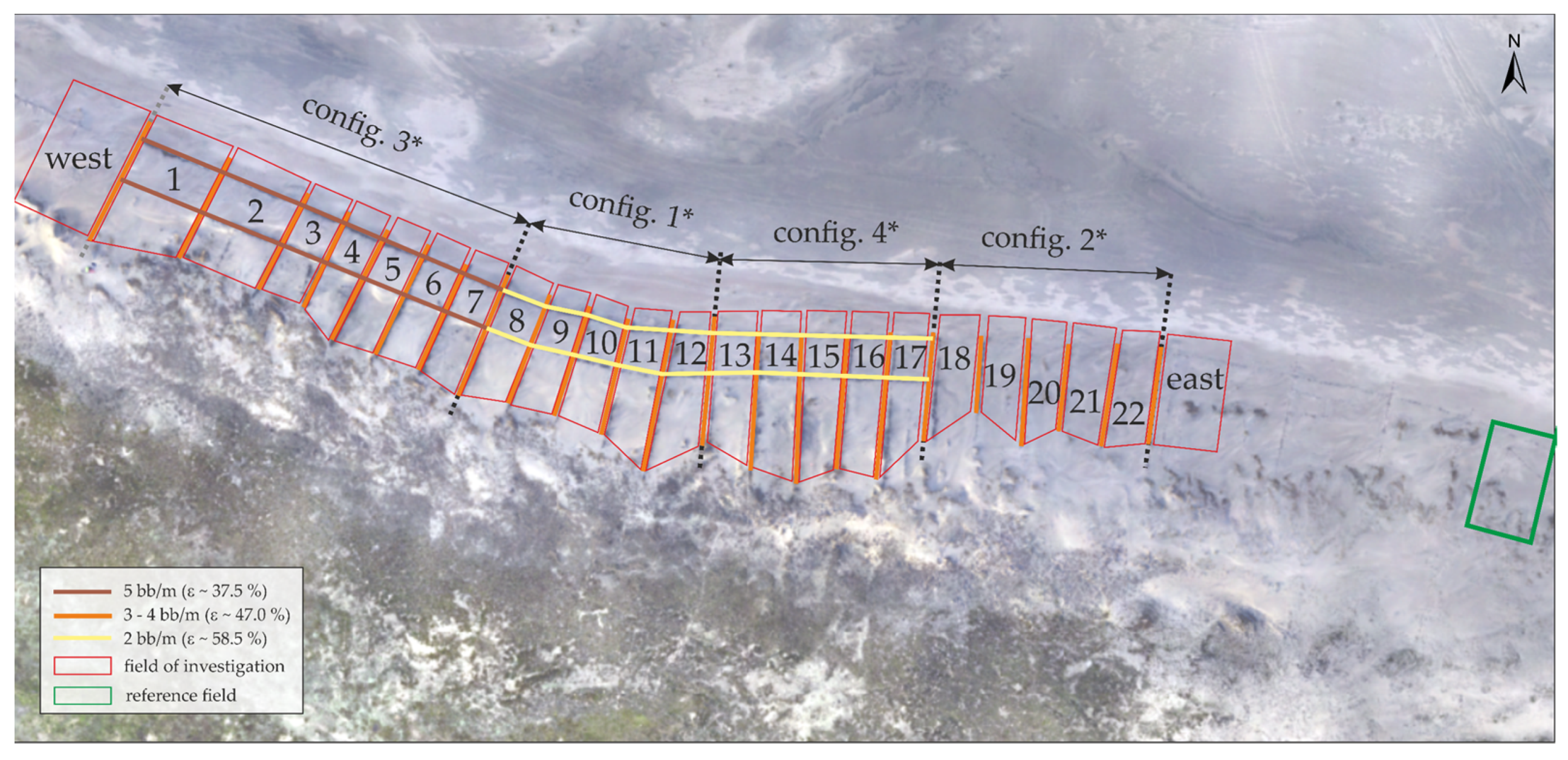
3.2. Sand Trapping Fence Configurations

Figure 4 shows an aerial drone photograph of the sand trapping fence at the dune toe at the study site of Langeoog. The sand trapping fence is stretched over a length of ~120 m and has four different configurations. The configurations differ in their arrangement of parallel and orthogonal brushwood lines to the coastal dunes and the number of bundles of brushwood used per running meter n [bb/m], see Figure 4. The red polygons delimit the individual fields 1–12, west, and east. A green polygon shows a field in which sediment deposition is not influenced by the sand trapping fence and which serves as a reference for further analysis. This reference field is located ~40 m east of field 12, ensuring that the sand trapping fence does not influence the wind field according to Dong et al. [28]. The sand trapping fence is characterized by thirteen brushwood lines (brown lines in Figure 4) arranged orthogonal to the coastal dunes and three brushwood lines (orange and yellow lines in Figure 4) parallel to the coastal dunes. The brushwood lines orthogonal to the coastal dunes have an average length of ~6 m, except for configuration 4, with an average length of ~3 m. There the deflectors at the dune toe are missing. Three parallel brushwood lines stretch over ~30 m each and intersect with the orthogonal brushwood lines. Configuration 1 consists of brushwood lines parallel (n = 2 bb/m) and orthogonal (n = 3–4 bb/m) to the coastal dunes. The westerly exposed configuration 1 is followed by configuration 2, consisting only of orthogonal brushwood lines (n = 3–4 bb/m) to the coastal dunes. Configuration 3 has the most densely set of parallel brushwood lines with n = 5 bb/m. Most eastward, configuration 4 lies with orthogonal brushwood lines with an average length of ~3 m. Offshore of the sand trapping fence Ammophila arenaria of varying heights (with a medium height of about 0.5 m) and irregularities in the topography were present in config. 2–4, see Figure 4. The vegetation covered maximum 3.0% of the investigated study area.

In Figure 5, an aerial drone photograph of the sand trapping fence at the study site of Norderney is shown. The red polygons delimit the individual fields 1–22, west, and east. A reference field, located ~75 m east of field 22, ensures no influencing effects of the sand trapping fence on the wind profile [27]. The reference field is located where the upper endings of brushwood lines of a sand trapping fence installed in the past exist. This sand trapping fence is already fully filled with sand, and the brushwood bundles protrude around 2–5 cm above the ground. Zhang et al. (2010) [26], from their findings in wind tunnel experiments, stated that behind a porous fence with a height of h = 3 cm, the saltating sand particles reach a maximum length of four times the fence height behind the porous fence in main wind direction for wind velocities up to u = 9 m/s. Even for higher wind velocities, see, e.g., NING et al. (2020) [32], who investigated the fence height effect on sand trapping in field experiments, it is assumed that the effect of this sand trapping fence is locally limited and therefore can be neglected for further analysis.

The sand trapping fence stretches over ~240 m. The configurations 1*, 2*, 3*, and 4* generally correspond to the configurations on Langeoog. However, for configurations 1*, 3*, and 4*, two parallel brushwood lines to the coastal dunes were installed, resulting in different field sizes between the brushwood lines. These fields are ~10 m wide, except for the first two fields in the west, which are ~20 m wide. The average length of the orthogonal brushwood lines is ~16 m. Furthermore, the arrangement of the configurations is different with configuration 3* followed by configuration 1*, configuration 4*, and configuration 2*, seen from west to east. When wind approaches from west or east, the outer fields have a potentially higher sediment supply since the sediment transport in the inner fields is attenuated by the brushwood bundles, resulting in a potentially lower sediment supply. Between the individual lines of brushwood only small spots of Ammophila arenaria, mainly in config. 4* and config 2*, were present, see Figure 5. The total coverage of the area with vegetation was maximum 3.5% at this study site.

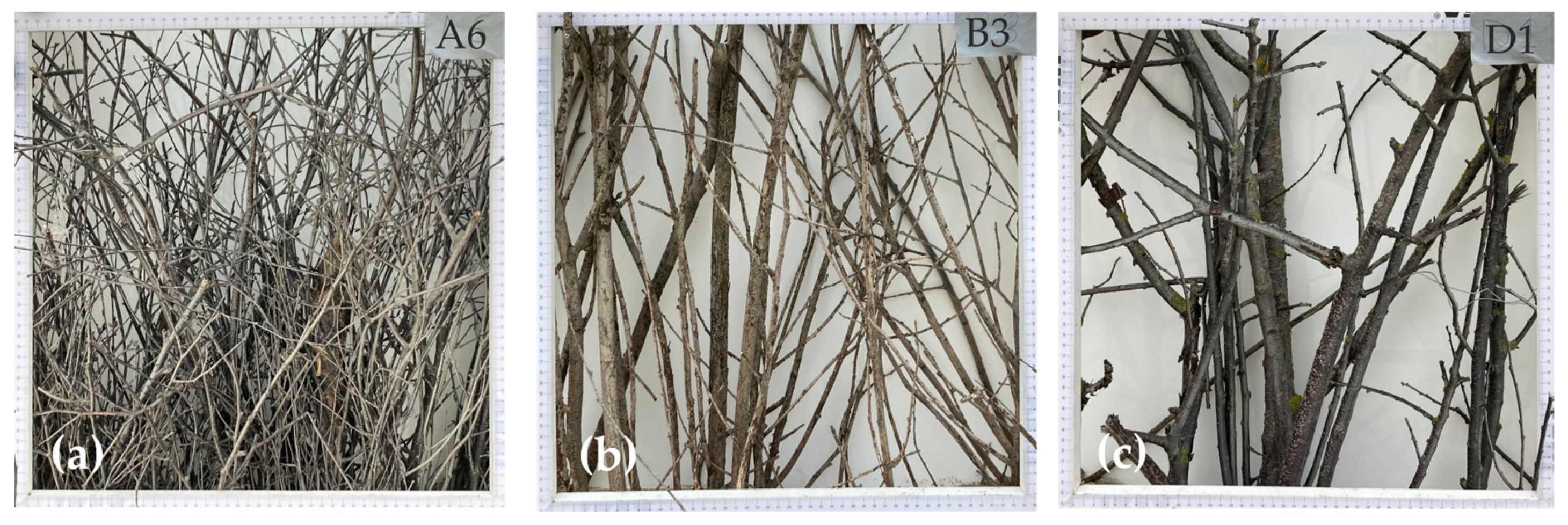
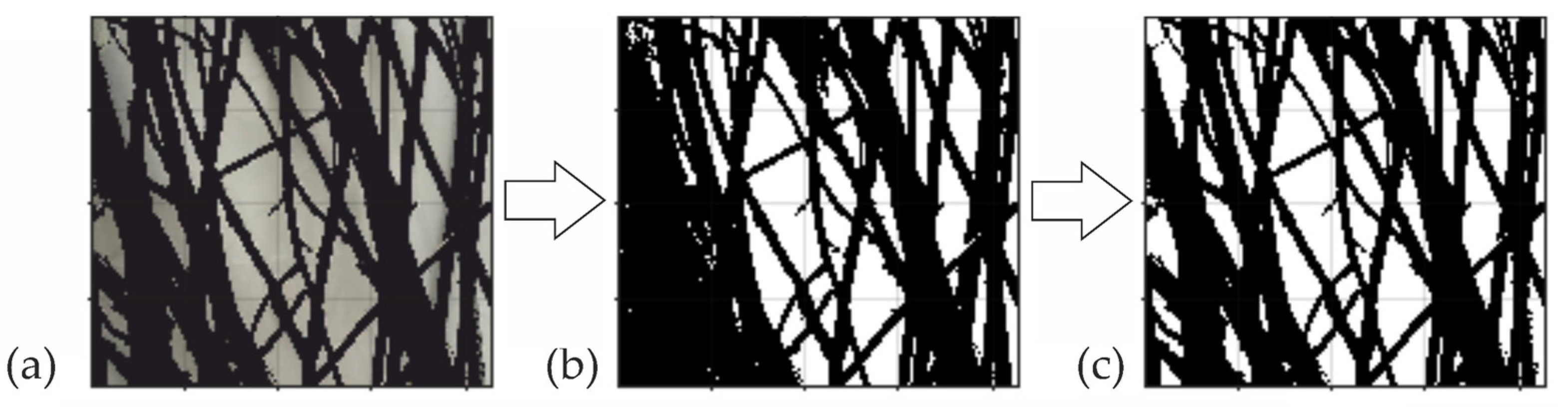
3.3. Sand Trapping Fence Porosity

In this section, the porosity of the sand trapping fences is determined, in addition to the number of brushwood bundles used per running meter n [bb/m]. It is necessary for the comparability of the results to determine the different porosities as the installation of the sand trapping fences was executed differently and furthermore, different types of branches were used, see Section 3.1, and therefore, the comparability of the results must be ensured.

In Figure 6, a standardized section of 45 cm × 45 cm of the sand trapping fence with (a) a low porosity with 5 bb/m, (b) a medium porosity with 3–4 bb/m, and (c) a high porosity with 2 bb/m is shown using the example of the study site Norderney.

The photographs were processed with the MATLAB (R2018b, version 9.510.944444) Color Thresholder Application [52]. The application offers four different color spaces for creating a mask to threshold the images. The color space red, green, blue (RGB) was chosen to create the masks, as the results were more precise than those obtained by the other color spaces. The color channel values, representing the color spaces of the brushwood bundles, were selected manually to segment the photographs. The image mask covers the regions overlaid by the brushwood branches in black, increasing the contrast to the background in white. Afterward, the masked images were converted into binary images. The small areas of black that were entirely surrounded by white color were removed to reduce the noise using the salt and pepper noise reduction filter [53]. The sand trapping fence’s porosity was determined by the ratio of black pixels of the noise-cleared image to the total number of pixels in the image [54]. Figure 7 shows (a) the masked image, (b) the binary image, and (c) the porosity clearance of the standardized section from configuration 2* of the sand trapping fence on Norderney with n = 3–4 bb/m.

The applied approach was validated by processing photographs of a defined number of brushwood branches (one up to five branches) with a known surface area. Therefore, the surface area was determined by measuring the length and width of the branches. As the branches show many irregularities in their geometry, the comparison between the results obtained by MATLAB and the measured lengths and widths contains uncertainties. However, with a mean error of the surface area error_mean ~ 0.11, a minimum error of error_min ~ 0.03, and a maximum error of error_max ~ 0.14, the applied approach shows good results for the validation case.

In

Table 1. Summary of sand trapping fence characteristics of Langeoog and Norderney comprising the date of installation of the sand trapping fence, the configuration type, the number of parallel brushwood lines to the coastal dunes k [-], the total length of parallel L₁ [m] and orthogonally L₂ [m] arranged brushwood lines, the number of used brushwood bundles for the parallel n [bb/m] and orthogonally i [bb/m] arranged brushwood lines to the coastal dunes, the dates at which the photographs were taken, the section of the sand trapping fence (lower or upper part), the average porosities of the brushwood bundles for the parallel ε_n [%] and orthogonally ε_i [%] arranged brushwood lines and the average porosity for each configuration $\overline{\epsilon }$ [%].

Study Site, Date of Installation	Config. Type	k [-]	L1+ L2 [m]	n [bb/m]	i [bb/m]	Date of Photograph	Section	εn [%]	εi [%]	$\overline{\mathit{\epsilon }} [\%]$
Langeoog, May 2020	1	1	30 + 24	~2	~3	26/05/2020 *	lower	33	24	29
	4		30 +15	~2	~3	26/05/2020 *	lower	33	24	30
	2		0 + 24	~3	~3	14/03/2021	upper	-	24	24
	3		30 + 24	~5	~3	26/05/2020 *	lower	12	24	17
Norderney, July 2020	1*	2	100 + 96	~2	~3–4	10/03/2021	upper	61	51	51
						01/08/2019 *	lower	49	43
							average	55	47
	4*		100 + 81	~2	~3–4	10/03/2021	upper	74	51	55
						01/08/2019 *	lower	50	43
							average	62	47
	2*		0 + 93	~3–4	~3–4	10/03/2021	upper	-	51	47
						01/08/2019	lower		43
							average		47
	3*		180 + 128	~5	~3–4	10/03/2021	upper	42	51	41
						01/08/2019 *	lower	33	43
							average	37.5	47

* Project partner NLWKN provided photographs.

, the date of installation of the sand trapping fence, the configuration type, the number of parallel brushwood lines to the coastal dunes k [-], the total length of parallel L₁ [m] and orthogonally L₂ [m] arranged brushwood lines, the number of used brushwood bundles for the parallel n [bb/m] and orthogonally i [bb/m] arranged brushwood lines to the coastal dunes, the dates at which the photographs were taken, the section of the sand trapping fence (lower or upper part), the average porosities of the brushwood bundles for the parallel ε_n [%] and orthogonally ε_i [%] arranged brushwood lines and the average porosity for each configuration $\overline{\epsilon }$ [%] are shown. The porosity was calculated out of several (between 4 and 21) photographs of the same configuration. The mean value of the porosity $\overline{\epsilon }$ [%] for each field of the sand trapping fence was determined from the porosities of the orthogonally and parallel brushwood bundles of this field, weighed by their length.

Note that the photographs were taken on different dates. As time progresses, more and more sand can accumulate at the brushwood lines of the sand trapping fence. Thus, the photographs taken later depict more of the upper section of the sand trapping fence, where the porosity is lower than the photographs taken earlier, which depict more of the lower section of the sand trapping fence, where the porosity is higher.

Generally, it becomes clear that with increasing brushwood bundles per running meter, the porosity decreases. What is striking in Table 1 is the difference between the determined porosities of the sand trapping fence on Langeoog and Norderney for the same configuration with an equal number of brushwood bundles per running meter. A possible explanation might be that different people installed the sand trapping fences, as discussed in Section 3.2. Furthermore, different types of brushwood bundles were used. The diversity of the brushwood bundles makes it challenging to build sand trapping fences with nearly identical characteristics. This underlines the importance of determining the porosity of the sand trapping fences to interpret their efficiency consistently. When comparing the individual islands to each other, it is better to compare the porosities instead of using brushwood bundles.

4. Materials and Methods

4.1. Experimental Instrumentation

The field campaigns employed an unmanned aerial vehicle (UAV, manufacturer DJI Phantom 4 with real-time kinematic). The UAV is equipped with a one-inch complementary metal-oxide-semiconductor sensor camera with a resolution of 20 megapixels to obtain ortho-image data and a real-time kinematic function to gain spatial coordinates. For detailed technical information on the UAV, the readers are referred to the drone’s user manual [55]. The UAV surveys were conducted on Langeoog from 20 May 2020 to 12 March 2021 and on Norderney from 24 August 2020 to 9 March 2021. The weather conditions were different from sunny and windless to stormy and cloudy.

Two flight plans on Norderney and four flight plans on Langeoog with varying flight altitudes between 20 m and 100 m (distance above the coastal dunes) were performed using the DJI Pilot app. The camera took photographs with 70% and 80% forward and lateral overlap, respectively. The flight velocity was kept low and varied around an average velocity of ~4 m/s.

The drone’s georeferenced ortho-images generally achieve an accuracy of 1 cm + 1 ppm (root mean square error) horizontally and 1.5 cm + 1 ppm vertically [55]. Four visible checkpoints were installed with coded target markers distributed within the study site to evaluate the precision of the derived digital elevation model (DEM). These checkpoints’ exact positions were also registered using the global navigation satellite system JAVAD GNSS Receiver SigmaD with an accuracy of 1 cm + 1 ppm (root mean square error) horizontally and 1.5 cm + 1 ppm vertically [56].

4.2. Structure from Motion Processing of UAV Images and Data Precision

The structure from motion processing of UAV images was performed using Agisoft Metashape Pro (version 1.6.5; 64 bit) [57] to obtain digital elevation models. The following steps were subsequently performed: (i) importing of photographs and camera positioning, (ii) conversion of the coordinate systems from Universal Transverse Mercator (UTM) World Geodetic System 1984 (WGS 84) with the geoid height Earth Gravitational Model 1996 (EGM 96) to UTM ETRS 89 with German Geoid height GCG 2016, (iii) image alignment at the high/highest accuracy level; (iv) gradual selection of study site, (v) checkpoint positioning, (vi) optimization of camera alignment, (vi) generation of the dense point cloud with high/medium accuracy and application of the moderate filter for calculating the depth maps, (vii) DEM and orthophotographs generation from the dense point cloud. The final UAV-derived DEM reached an averaged resolution of ~3.5 cm/pixel. Additionally, the measured checkpoints gave coordinates in UTM WGS 84 with ellipsoidal heights converted into UTM ETRS89 with GCG 2016 heights.

The difference in x-, y-, and z-direction between the markers in the DEM obtained by the UAV and the measured checkpoints gave mean distances for the study site Langeoog of 0.023 m, 0.032 m, and 0.059 m for x, y, and z, respectively. For Norderney, the UAV flew at higher altitudes, resulting in mean distances of x = 0.051 m, y = 0.047 m, and z = 0.085 m.

4.3. Analysis Method for Evaluating the Dune Toe Growth

The coastal beach-dune system can be divided into five cross-shore horizontal elevation slices: (1) bed, (2) foreshore, (3) intertidal beach, (4) dry beach, and (5) coastal dunes with (6) sand trapping fence, see Figure 8. The dune toe level separates the dry beach (5) from the coastal dunes (5). The dune toe level at the East Frisian Islands is defined at z = +3 mNHN [49].

In the following, the dune volume (7), see Figure 8, was defined as the volume of sand above a fixed horizontal plane in the z-direction and a vertical boundary in the x-direction (approximately ~3 m onshore of the orthogonal deflectors of the sand trapping fence). In addition, the horizontal z-plane was chosen to be at least at dune toe level and at the same time ~3 m onshore of the sand trapping fence’s deflectors, see Figure 4 and Figure 5. Thereby, it was ensured that the sand trapping fences directly influence the observed study site at the dune toe.

Therefore, the chosen dune volume is defined depending on the chosen boundary planes and does not represent the whole coastal dune volume.

In addition to calculating the dune volume around the sand trapping fence, the dune volume between the orthogonally arranged brushwood lines was also determined for each field individually. Thereby, a comparison of the different configurations to each other is possible.

The dune volumes at different times were calculated using ArcGIS (version 10.5.1; 64 bit) [58]. For this purpose, the formatted. xyz digital elevation model derived from Agisoft Metashape Pro [57] was converted to a database, added to the map as a layer, and the obtained multipoint input features were converted to a raster. Afterward, shape polygons were defined for the different areas of interest, and then the three-dimensional (3D) Analyst surface volume tool was applied to obtain the dune volumes over a standardized section V/A [m³/m²]. Finally, the interpolate shape tool was used to obtain the cross-sectional and longitudinal dune profiles.

4.4. Calculation Procedure of Potential Aeolian Sediment Transport

The saturated aeolian sediment transport rate q_s [kg/m/hr] is calculated by a modified Bagnold model [21,59]:

$$q_s=\{\begin{array}{cc}3600·{\alpha }_B·\sqrt{\frac{d_{50}}{d_{50,ref}}}·\frac{{\rho }_a}{g}·\left(u_{*}{}^3-u_{*t}{}^3\right)\hfill & \hfill for u_{*}>u_{*t}\\ 0& for u_{* }>u_{*t}\hfill \end{array}$$

(1)

For the Bagnold factor, a value of α_B = 2 was chosen to represent naturally graded sand [21,22]. The mean particle size was defined with d₅₀ = 218 µm [36], and the reference sediment diameter was d_50,ref = 250 µm as a standard value for dune sand [60]. The air density was chosen as ρ_a =1.2 kg/m³ and the gravitational acceleration as g = 9.81 m/². u_* [m/s] is the shear velocity and u_*t [m/s] is the critical shear velocity, at which transport of dry sand is initiated [18]. The shear velocity is assumed to be constant over an hourly interval. According to Sarre (1989) [61], these simplifications in the determination of potential aeolian transport rates are not critical, whereas other transport-limiting factors, such as surface moisture or vegetation, are of greater importance in coastal areas [6]. Except for wind velocity, all parameters in Equation (1) are considered constant over time. It implies that the sediment transport rate depends solely on the variability of the wind [22,60,62,63].

The potential transport rates represent the maximum transport rates as transport limiting factors like surface roughness, vegetation, shells, surface slope, and fetch effects are neglected [59,62,64,65,66]. The fetch effect increases sediment transport rates with increasing fetch length downwind until an equilibrium condition is reached. Thus, a fetch length shorter than the critical fetch length can result in lower transport rates [65,67]. On narrow beaches, the critical fetch is often not reached, leading to limited aeolian sediment transport conditions depending on the incoming wind direction [50,68]. Numerous authors found that the critical fetch distance F [m] ranges from seven to tens of meters [7,65,69,70,71]. As the dry beach widths of Norderney W ~ 320 m and Langeoog W ~ 70 m were wider over the measuring period than the critical fetch distance with F ~ 50 m, see Section 2, we assume no influence on potential sediment transport by reduced fetch lengths.

It is necessary to know the aerodynamic roughness length or a measured vertical wind profile to determine the shear velocity [72]. However, since the roughness length varies temporally and spatially, it is not useful to use it for this work [72,73]. In contrast, Hsu (1974) [74] proposed the following relationship for predicting shear velocity for dry beach areas from routine hourly wind observations at meteorological weather stations:

$$u_{*}=0.037·u_{10}.$$

(2)

The wind velocity measured 10 m above ground is given with u₁₀ [m/s]. The equation is based on field data from numerous study sites [5,74]. The critical shear velocity is given with:

$$u_{*t}=A·\sqrt{\left(\frac{{\rho }_s}{{\rho }_a}-1\right)·g·d_{50}},$$

(3)

where A [-] is an empirical constant (here: 0.11) [21,75] and ρ_s = 2650 kg/m³ is the density of sand grains. With the given parameters for Langeoog [36], the critical shear velocity at the study site can be calculated as u_*t = 0.24 m/s. Since Langeoog and Norderney are sedimentologically similar, the same mean grain size and the same critical shear velocity is assumed for Norderney, respectively.

The sum of the potential transport rates calculated accordingly to Equation (1) over the measured time series gives the total sediment transport depending on the angle of prevailing wind direction relative to the coastline. For total cross-shore sediment transport Q_cross-shore [m³/m], see Equation (4), and for total longshore sediment transport Q_longshore [m³/m], see Equation (5):

$$Q_{cross\text{-}shore}=\frac{1}{{\rho }_b}{\displaystyle \sum }_{i=1}^k{q}_i·\sin \left(\gamma -O\right)=\frac{1}{{\rho }_b}{\displaystyle \sum }_{i=1}^k{q}_i·\sin \left(d{d}_j\right)$$

(4)

$$Q_{longshore}=\frac{1}{{\rho }_b}{\displaystyle \sum }_{i=1}^k{q}_i·\cos \left(\gamma -O\right)=\frac{1}{{\rho }_b}{\displaystyle \sum }_{i=1}^k{q}_i·\cos \left(d{d}_j\right)$$

(5)

where γ [°] is the angle between wind direction and north, O [°] is the orientation of the coastline, dd_j [°] is the difference between the wind direction and the coastal orientation, and ρ_b [kg/m³] is the bulk density of sand. The bulk density ρ_b = 1600 kg/m³ was chosen as van Rijn (2019) [59] used the value for the Dutch coast and Strypsteen (2019) [5] for the Belgian coast. The total number of hours in the measured time series is represented by k [-] [5,76]. To compare predicted potential dune volume changes (as a function of potential sediment transport) with measured dune volume changes, the angle of the wind to the coastline is considered by the sinus and cosine function. In Figure 9, the explained approach is applied for both study sites showing the different angles. For the coastline of Langeoog and Norderney, an orientation of O_Langeoog = 88° and O_Norderney = 110° to the north is assumed, respectively.

5. Results and Discussion of Topographic Data

5.1. Dune Volume Changes

Figure 10 shows the orthophotographs with elevation heights ranging from 3 mNHN up to 8 mNHN of Langeoog’s sand trapping fence on 20 May 2020, 15 June 2020, 27 August 2020, 26 October 2020, 14 December 2020, and 12 March 2021. As the terrain surface height increases, the colormap changes from (light) green to (light) orange to red. The upper boundary of the green area to the north represents the dune toe level. Immediately after finishing the construction of the sand trapping fence on 19 May 2020, the first drone survey was conducted on 20 May 2020. Therefore, Figure 10a, represents the initial condition of the dune volume at the dune toe. In Figure 10b–f, sand has accumulated at the brushwood lines of the sand trapping fence as time passes.

Figure 10 shows that the terrain elevation’s continuous and relatively uniform growth is evident from the contours parallel to the coastal dunes. Furthermore, it seems that the coastal dunes in the west are already more developed compared to the coastal dunes in the east. It becomes clear that the dune toe level continued to move towards the North Sea at least 0.3 m but at most 3.9 m. Especially during late autumn, the individual fields between the brushwood lines were filled with sand.

To highlight the areas of sedimentation and erosion, Figure 11 shows the different elevation heights derived from the DEM of the study site of Langeoog from 20 May 2020 compared to 12 March 2021. Areas of erosion are displayed in blue colors, whereas sedimentation areas are shown in red colors. The white colors indicate areas where the elevation change is smaller than the threshold of measurement uncertainty (~10 cm).

It is clearly visible that a particularly large amount of sand accumulated at the individual lines of brushwood of the sand trapping fence. Large areas on the beach, onshore of the sand trapping fence, have grown as time passes, initiating the dune toe growth. Over the measured time period, the surface elevation grew up to Δh_max = +1.75 m. However, erosion areas also exist on the beach onshore and offshore of the sand trapping fence (Δh_min = −1.25 m), see Figure 11. The different configurations have each experienced varying degrees of growth:

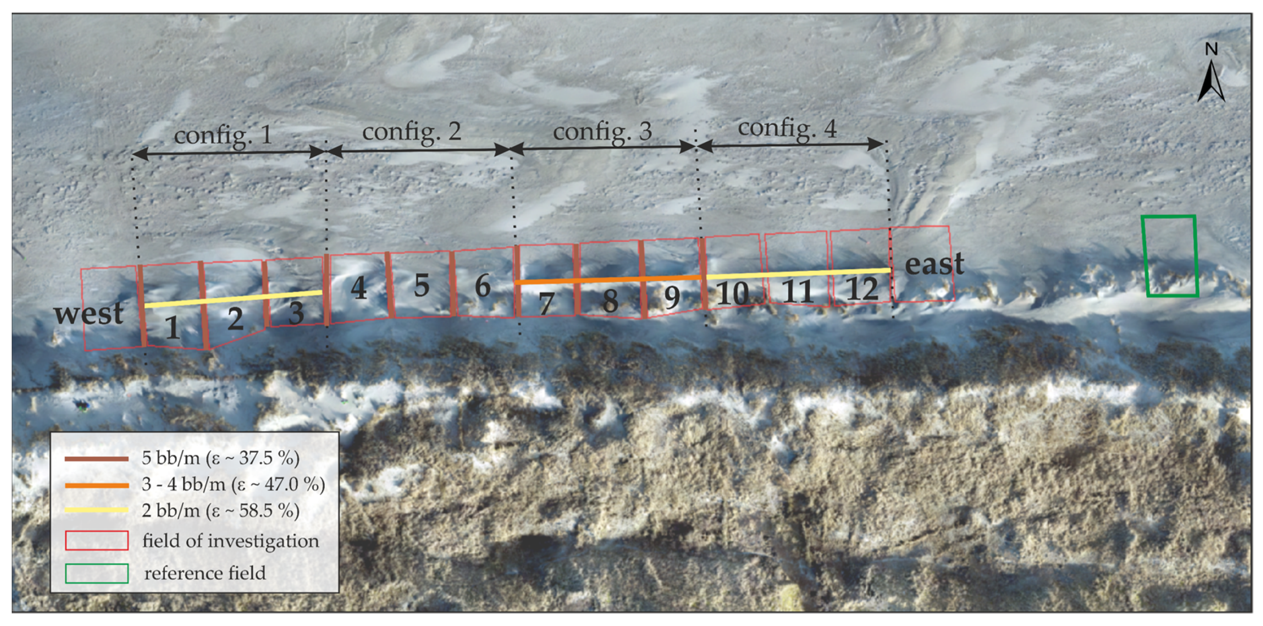
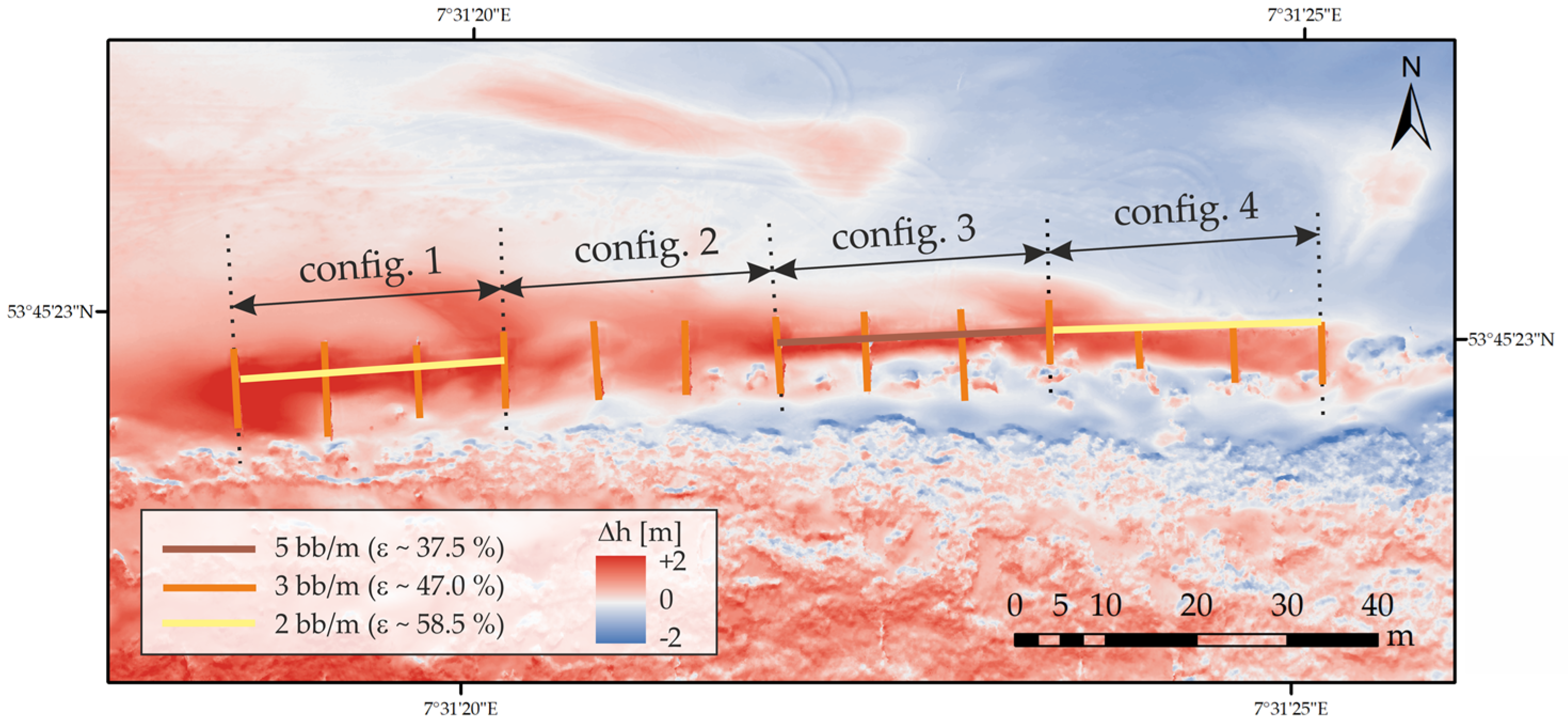
• Configuration 1: In the first three fields to the west, an average sand volume of ΔV/A_config.₁ ~ 0.71 m³/m² has accumulated over the whole time period, implying that the amount of accumulated sand is 13% higher compared to the mean of all configurations (ΔV/A_config._1–4 ~ 0.63 m³/m²). The first field exposed to the west trapped the highest amount of sand with ΔV/A_field1 ~ 0.80 m³/m² (Δh_field1 = + 1.75 m). As time passed, sand has accumulated both at the parallel and orthogonal lines of brushwood and onshore of the sand trapping fence’s deflectors, meaning that the dune toe shifted onshore towards the north.
• For configuration 2, only moderate accumulation of sand up to Δh_config._2,max = +1.39 m has occurred at and between the orthogonally arranged deflectors and onshore of the sand trapping fence close to the dune toe. An average sand volume of ΔV/A_config.₂ = 0.60 m³/m² has accumulated over the measuring time.
• Configuration 3: Predominantly, sand has accumulated at the parallel lines of brushwood and the onshore deflectors. There is hardly any accumulation present offshore of the parallel brushwood lines towards the coastal dunes. Thus, areas of erosion are more likely to be found here. This configuration recorded the lowest growth over the whole measuring time with a sand volume of ΔV/A_config.₃ = 0.56 m³/m². The sand accumulated up to Δh_config.₃ = +1.42 m.
• For configuration 4, extensive growth of the sediment pockets between the orthogonally arranged brushwood bundles offshore of the parallel brushwood line has been recorded, with heights up to Δh_config._4,max = +1.25 m. The sand volume on the lee side grew faster than the dune volume on the luv side. The configuration has the second-largest growth rate with an accumulated sand volume of ΔV/A_config.₄ = 0.66 m³/m² over the measured time. However, there are extensive erosion areas on the beach, and the dune toe level has not increased significantly.

A closer look at the standardized sand volume changes per defined area at each measuring time shows that the different configurations differ in the amount of accumulated sand, see Figure 12. For configuration 1–4, the results are shown as boxplots containing three fields for each configuration, in Figure 12a–d. The red lines within the boxplots represent the median values of dune toe volume change. In Figure 12e, the fields west and east, and in Figure 12f the reference field is shown, respectively.

The measured values were connected linearly over time, even though this may deviate from reality. However, no measurement results are available for the time interval between, and thus, the trend of the volume changes at the sand trapping fence becomes visible.

The growth rate for all areas was highest from 27 August 2020 to 26 October 2020 and 14 December 2020 to 12 March 2021, whereas only small growth rates were present from 15 June 2020 to 27 August 2020. The areas in the west of the sand trapping fence and of configuration 1 increased over the entire measurement period, whereby the field exposed to the west had a more substantial increase at the beginning during summer compared to configuration 1 and a lower increase from 14 December 2020 to 12 March 2021.

The areas east of the sand trapping fence and configurations 2–4 showed a very similar trend: firstly, slight sedimentation occurred, followed by erosion processes from 15 June 2020 to 27 August 2020. A renewed increase, which stagnated in the meantime (26 October 2020 to 14 December 2020), then increased until 12 March 2021 again, followed. The sand volume of configuration 4 almost reached the final dune volume of configuration 1.

Figure 4f shows the amount of sand deposited at the study site without a sand trapping fence, which during the whole period of the investigations amounts to V/A ~ 0.2 m³/m². This might be due to the natural development of the coastal dunes. Comparing the results of the reference field, see Figure 4f, to the results of the other fields, it is noted that the sand trapping fence has a positive influence on trapping sand at the dune toe as much more sand has been trapped at the brushwood lines than without any brushwood bundles. The reference field has a similar volume change over time compared to the east field. This indicates that, directly east of the sand trapping fence, its effect on the deposition of sediment has already vanished.

The coastal dunes are already more established at the eastern end than the western end, see Figure 13. This might explain more rapid growth at the western end than at the eastern end, given that dune growth tends to follow a sigmoid growth curve [12,77]. Houser et al. (2015) [77] conducted field measurements at the northern Gulf of Mexico (Santa Rosa Island, Florida and Galveston Island, Texas) and found that for predicting the evolution of a barrier island’s foredune height a parameterized sigmoid growth curve can be applied. These results are supported by Dalyander et al. (2020) [12], who developed an empirical dune growth model to predict the evolution of the foredune of a barrier island for the example of the Dauphin Island (Alabama). This could influence the observed variability in sediment accumulation independently of the sand trapping configurations.

Figure 13 shows the orthophotographs with elevation heights ranging from 3 mNHN up to 8 mNHN of Norderney’s sand trapping fence on 24 August 2020, 12 December 2020, 09 March 2021, respectively. The first orthophotograph from 27 August 2020 depicts the sand trapping fence’s condition approximately one year after its installation. At this date, sand has already been deposited at the sand trapping fence.

Figure 13 reveals an increase in the dune toe level from 24 August 2020 to 9 March 2021. The dune toe level shifted onshore towards the north, a minimum of at least 0.2 m and a maximum of 2.9 m.

Over the measured time period, the surface elevation grew up about Δh_max = + 1.20 m, see Figure 14. Only little areas directly along the brushwood lines offshore show erosion, see Figure 14. The different configurations have experienced the following degrees of growth:

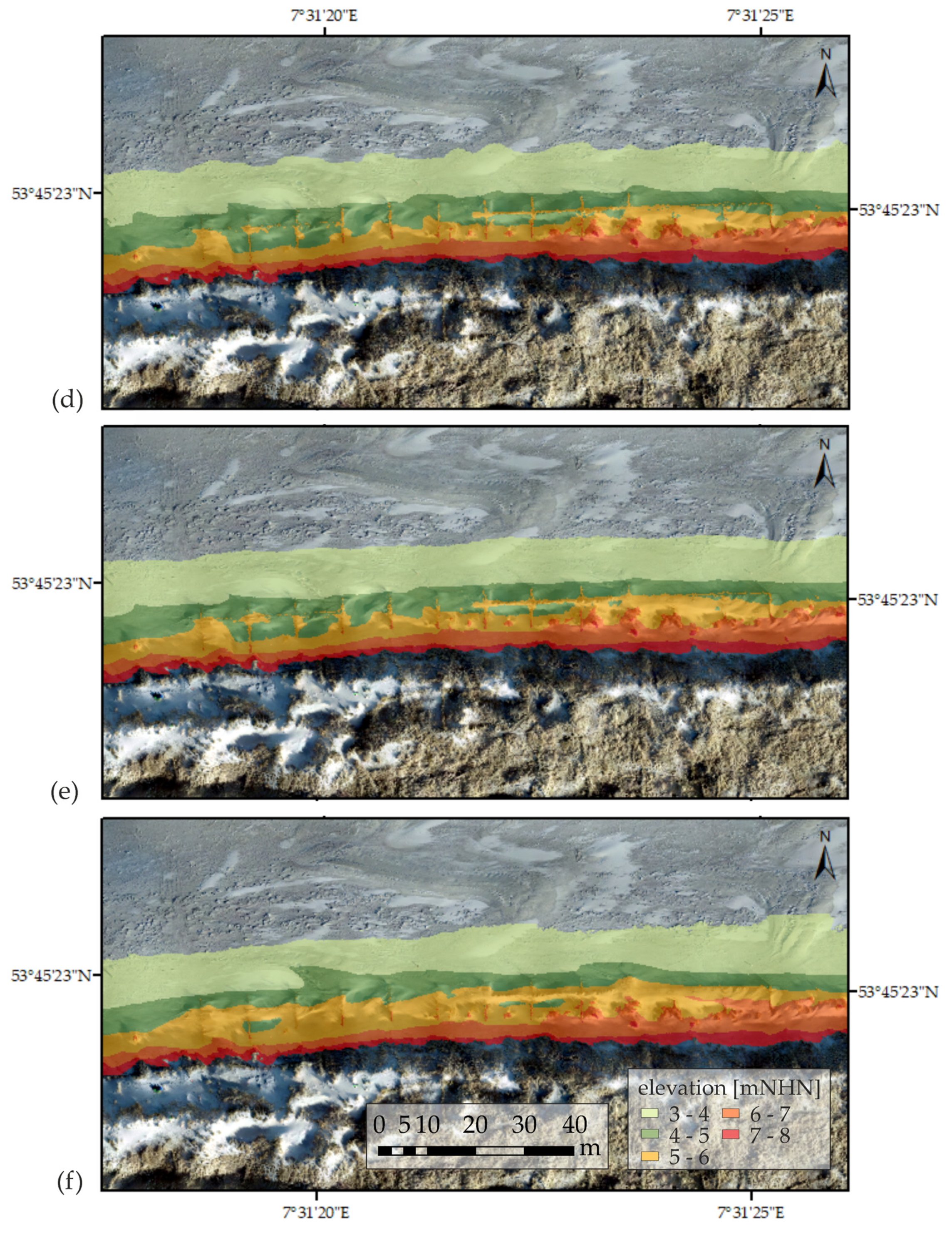
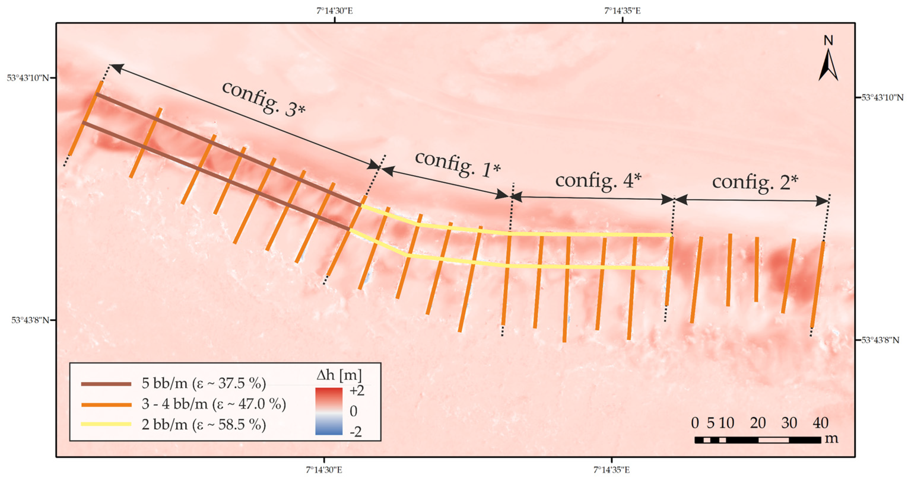
• Configuration 3*: The area onshore of the sand trapping fence on the beach and between the two parallel brushwood lines has grown significantly. The areas offshore of the second parallel brushwood lines are essentially unchanged. Only the field exposed to the west shows accumulated sand. The growth for configuration 3* was generally very homogeneous with heights up to Δh_config._3*= + 1.16 m. A sand volume of ΔV/A_config._3* = 0.18 m³/m² has accumulated over the measuring time.
• Configuration 1* recorded the lowest sand volume change with a value of ΔV/A_config._3* = 0.04 m³/m² over measuring time. Both onshore and offshore fields have developed very similarly over time. The dune toe level increased significantly over the measuring time.
• Configuration 4*: A sand volume of ΔV/A_config._4* = 0.09 m³/m² has accumulated over the whole measuring time. The development of the fields largely corresponds to the development of configuration 1*, whereas the dune toe level increased less.
• In configuration 2*, a sand volume of ΔV/A_config._2* = 0.27 m³/m² has accumulated over the measuring time. The dune toe level has grown only a little. The fields between the orthogonal brushwood lines were filled homogenously, whereby the fields exposed to the east recorded the most significant increase with Δh_config._3* = + 1.20 m.

Figure 15 shows the corresponding standardized sand volume changes per area at each measuring time for Norderney.

In general, the trends of sand volume changes are very similar for all configurations. From 25 August 2020 to 12 December 2020; a slight stagnation or even a decrease in the sand volume occurred. It is followed by a considerable increase in sand volume from 12 December 2020 to 09 March 2021, with the most substantial increase for configuration 2* and configuration 3*. These configurations with the fields in the west accumulated the most sediment in total.

The reference field without any sand trapping fence, see Figure 5, shows a similar trend of volume change over the measurement period as for the east field. The comparison between the reference field without any sand trapping fence and the fields with sand trapping fence confirm the effectiveness of the sand trapping fences to initiate the growth of the dune toe.

When evaluating the sand volume changes of the different configurations on Norderney and Langeoog, the different initial and boundary conditions have to be considered. Therefore, the results of both study sites are not directly comparable: firstly, the configurations are arranged differently to each other depending on their location, see Section 3.2. Secondly, Langeoog’s and Norderney’s coastlines are orientated differently to the north, see Figure 9, resulting in different onshore and longshore wind conditions, see Figure 3. In addition, the beaches have different profiles and are different in size, see Section 3.1. The investigated sand trapping fence on Norderney are directly surrounded by earlier installed sand trapping fences whereas, on Langeoog, the next sand trapping fence is several hundred meters away. As stated above, the sand trapping fence on Norderney was established earlier than on Langeoog, and therefore, any incipient coastal dune growth has likely already occurred, explaining slower growth rates.

Moreover, the effectiveness of the sand trapping fence is influenced by independent morphological events such as the migration of ridges. For example, on Langeoog, it can be seen that erosion took place on the beach and, thus, resulted in potentially lower sand volume changes close to the erosive area of the beach, see Figure 11.

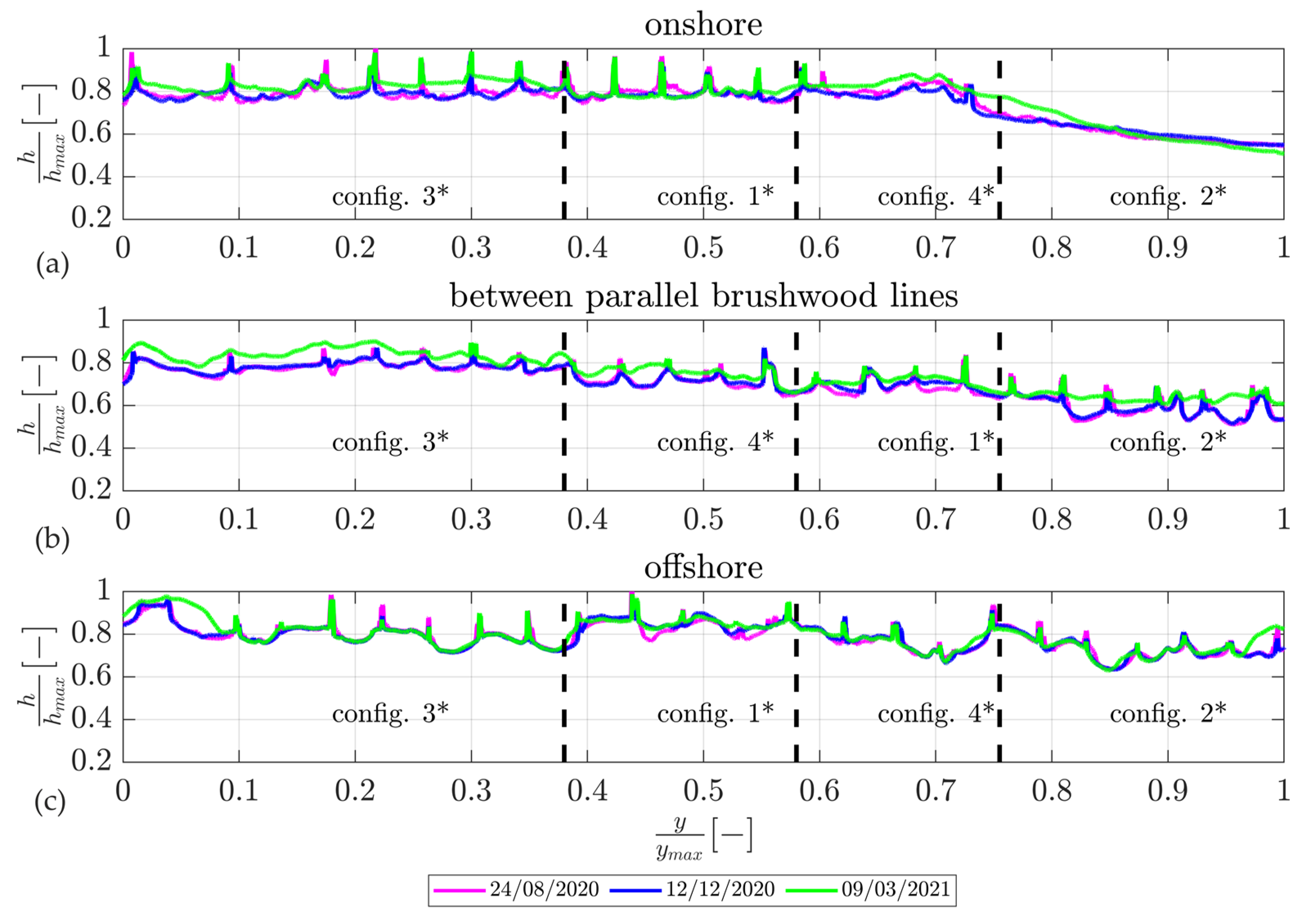
5.2. Development of the Longshore Dune Profile Influenced by Sand Trapping Fences

Figure 16a shows the longshore dune profiles onshore and Figure 16b offshore of the sand trapping fence of the study site Langeoog on 20 May 2020, 15 June 2020, 27 August 2020, 26 October 2020, 14 December 2020, and 12 March 2021. The y-axis shows the distance alongshore, and the z-axis the height. Both distances are standardized along their individual maximum length and height, respectively. The dashed lines in Figure 16 indicate the brushwood lines arranged orthogonal to the coastal dunes.

The following can be seen even more clearly: firstly, the sand accumulates at the brushwood lines upwards before the sand accumulates in width, as also observed by Ning et al. (2020) [31]. Exposed fields with potentially higher sediment transport brushwood lines can trap more sand than other fields without any exposed position.

In Figure 17, onshore fields show higher growth compared to the offshore fields. Areas that have grown remarkably onshore are not necessarily areas with significant growth offshore. Configuration 4* has experienced the most growth of all configurations.

It becomes clear that growth has occurred primarily from 12 December 2020 to 09 March 2021. The area between the two parallel brushwood lines, see Figure 17b, has grown, particularly in configuration 3* and configuration 2*.

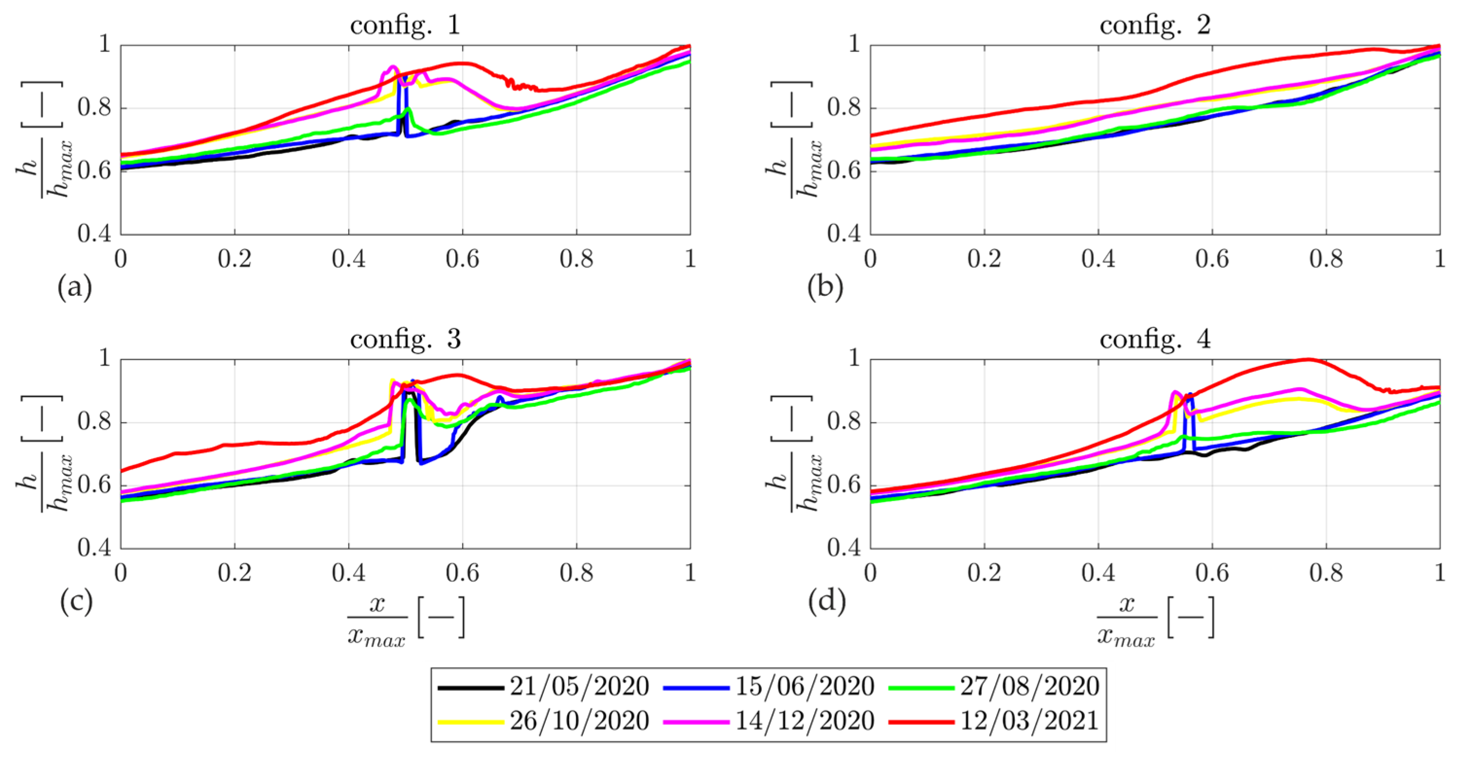
5.3. Development of the Cross-Shore Dune Profile Influenced by Sand Trapping Fences

Figure 18 shows the cross-shore dune profiles of all four configurations over the measuring period. A representative cross-shore profile positioned in the middle of a field for each configuration is displayed. The cross-shore distance and the height are standardized along their individual maximum length and height, respectively. For configurations 1, 2, 3, the cross-shore brushwood lines can be recognized at about half of the distance cross-shore. Configuration 2, however, has no cross-shore brushwood lines.

Configuration 2 indicates a relatively continuous growth in height distributed cross-shore. Configurations 1–3 show very similar growth, with configurations 1 and 3 showing more growth onshore than offshore. Configuration 4 shows especially growth offshore towards the coastal dunes.

In Figure 19, the cross-shore dune profiles for the study site Norderney are shown, respectively.

For configuration 2*, the growth occurred in the natural dune shape. Configurations 1*, 3*, 4* show very similar dune growth. First, the area offshore is filled with sand, propagating onshore. Configuration 4*, without any orthogonally arranged deflectors at the dune toe, showed a slower increase in the dune toe level compared to the other configurations.

The brushwood lines arranged parallel to the coastal dunes with higher porosity (see Figure 4 and Figure 5) have allowed growth further in cross-shore direction than those with lower porosity, where local growth directly at the brushwood line has been greatly increased. Furthermore, it is suggested that the orthogonally arranged deflectors at the dune toe favour an accretion of sand at the dune toe.

6. Discussion

The spatial distribution of the vegetation Ammophila arenaria and the ratio of vegetated and total area were determined by using ArcGIS (version 10.5.1; 64 bit) [58]. With the help of orthophotographs, vegetation was identified and its area share was calculated. During the measurement period, the vegetation cover varied between 0.8–3.0% (Langeoog) and between 1.2–3.5% (Norderney), respectively. As generally acknowledged in the literature, the presence of vegetation significantly affects sand trapping at coastal foredunes by increasing the surface roughness, which promotes sediment deposition and incipient dune formation [30,78,79,80,81]. There is a strong correlation between dune morphodynamic and vegetation, which considerably varies in time and space due to influencing factors such as rainfall or temperature [37,82,83]. As the vegetation area is locally limited and relatively scarce for both study sites, we expect this to have little effect on the sediment deposition as compared to the effect of the sand trapping fence.

The brushwood bundles on both study sites differ from each other in their porosity and stem characteristics, especially stem diameter, see Section 3.1. At present, we are not aware that the stem diameter has a significant influence on sediment transport and subsequence trapping efficiency, especially since, in scientific research, the fence’s porosity was identified as the major influence on these parameters (e.g., [25,26,32,79,84]).

Beach nourishments usually enlarge the beach width and thereby the fetch length over the beach increases as well [85]. Furthermore, rates of aeolian sediment transport depend on the grain size and the amount of shell fragments [85,86], see Equation 1 and Equation 3. This means that, e.g., coarser grains would lead to a potentially lower sediment transport rate. Since many long-term effects of nourishments are still not fully understood, these nourishments could influence the development of the coastal dunes [6,9]. This, in turn, leads to further uncertainty in calculating the potential sediment transport rates, see Figures 21 and 22, since beach nourishments are not considered in these calculations. However, their influence is expected to be only small since over the measuring period, the fetch length was always greater than the critical fetch length. Furthermore, the sediment supply was sufficient for aeolian sediment transport before and after the beach nourishments took place.

Another uncertainty when discussing the results is the natural development of coastal dunes [77]. This phenomenon can superimpose or interact with the trapping efficiency of newly installed sand trapping fences.

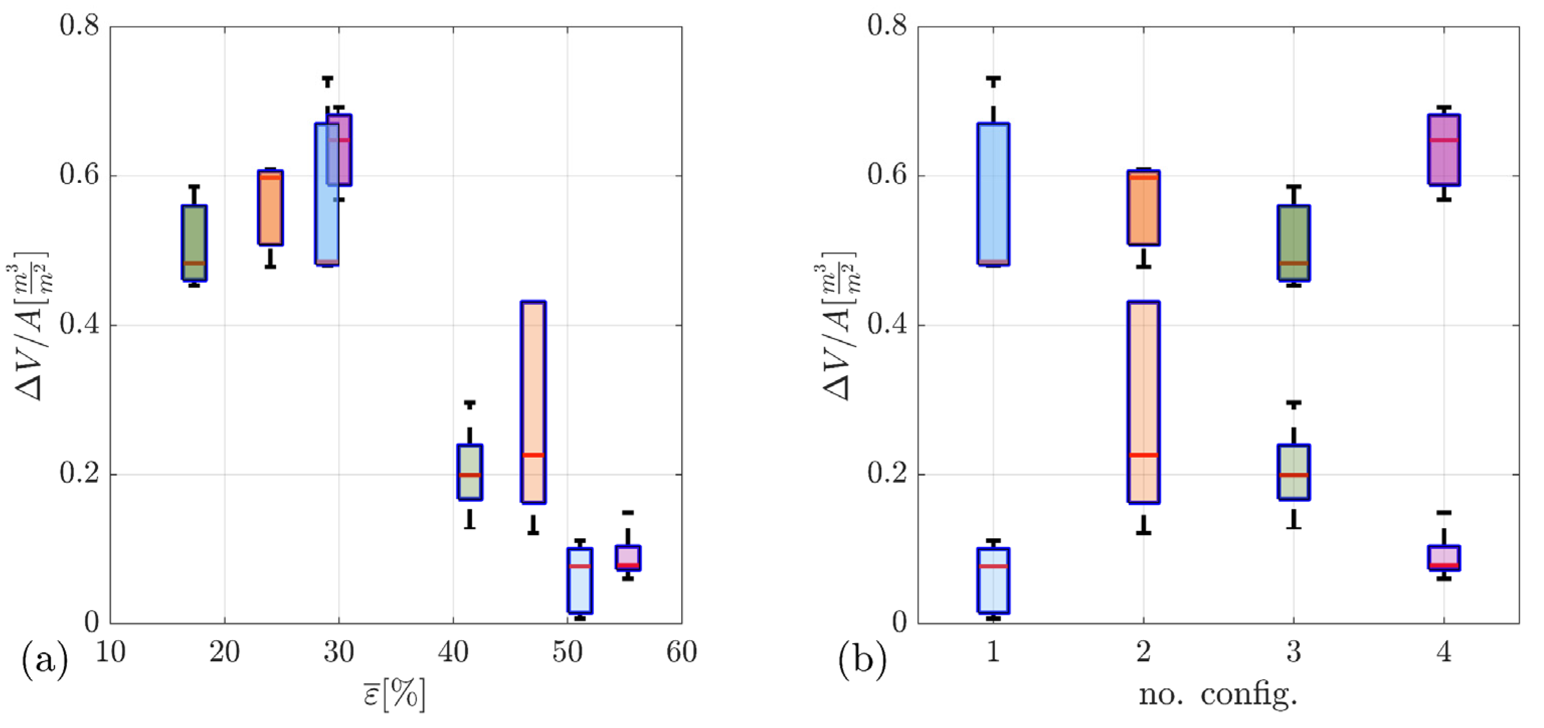
6.1. Trap Efficiency of Different Sand Trapping Fence Configurations

In Figure 20, the sand volume changes from August 2020 to March 2021 (197 days) on Langeoog (dark colors) and Norderney (light colors) are shown. On the y-axis the sand volume changes per square meter over 197 days are shown. On the x-axis in Figure 20a the average porosities $\overline{\epsilon }$ [%] of parallel and orthogonal brushwood lines are shown, whereas in Figure 20b the x-axis depicts the configuration number. The outwardly exposed fields showed a particular large accumulation of sand, see Figure 12 and Figure 15, most likely due to the increased supply of sediment compared to the other fields.

It can be seen in Figure 20a that, for configurations 1–4, a greater dune toe growth was recorded than for configurations 1*–4* comparing the same time period from August 2020 to March 2021. Norderney shows significantly lower sand volume changes over time than Langeoog. It seems reasonable that the potential growth rate is particularly high directly after finishing the construction of a new sand trapping fence like on Langeoog because the branches stick out high from the sand and have a lower porosity near the ground, see Section 3.3. As time passes, more sand has already accumulated at the brushwood lines, meaning that only the upper part of the sand trapping fence with a higher porosity sticks out at the top. This probably slows down the growth rate.

In Figure 20b, the sand volume changes are plotted over the different configurations, showing that a similar configuration on Langeoog leads to a different result on Norderney. This implies that the prevailing boundary conditions like sediment supply or the age of the installed sand trapping fence (height and porosity of the remaining branches) have a strong influence on the different configurations’ effectiveness, see also Section 5.1.

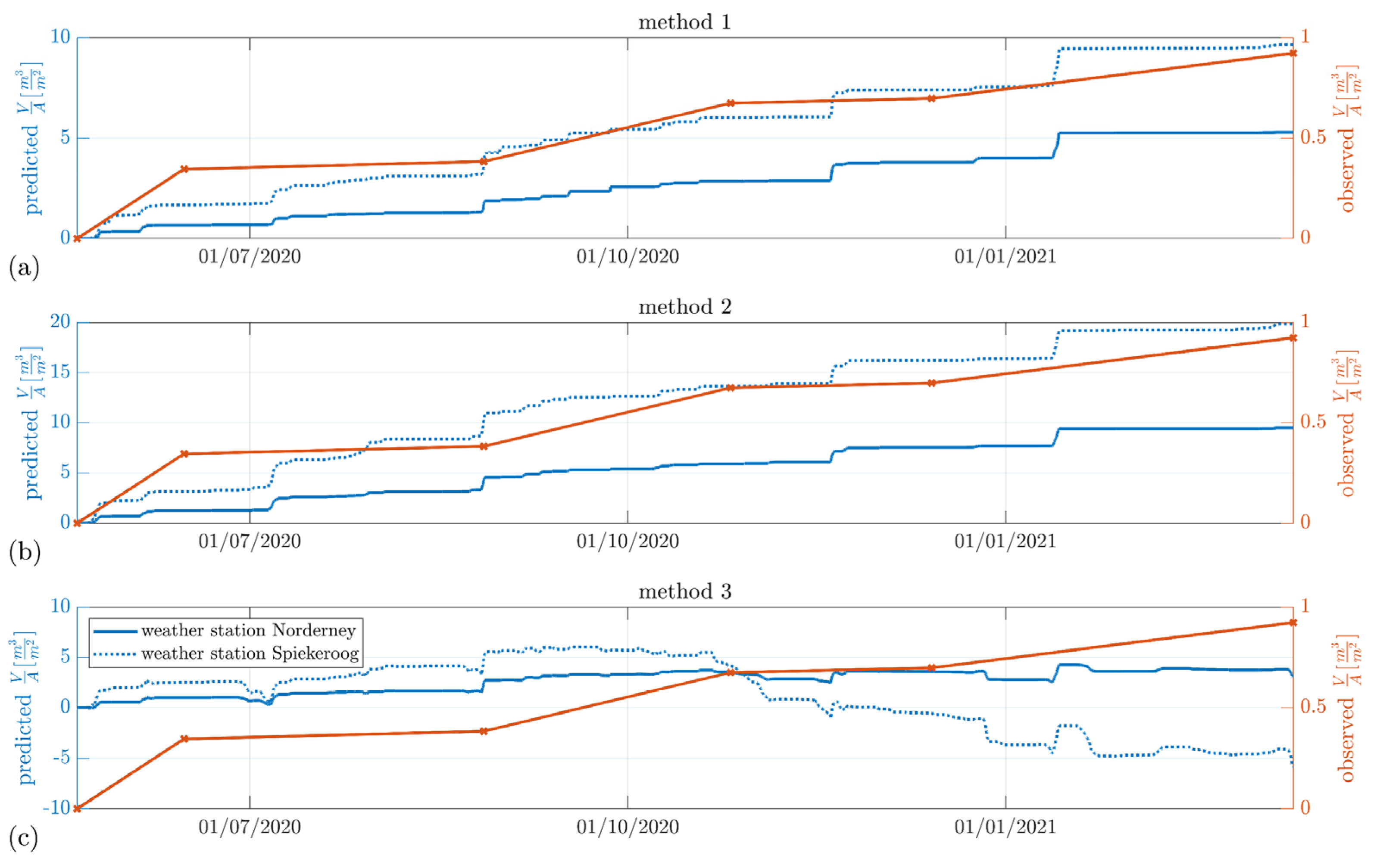
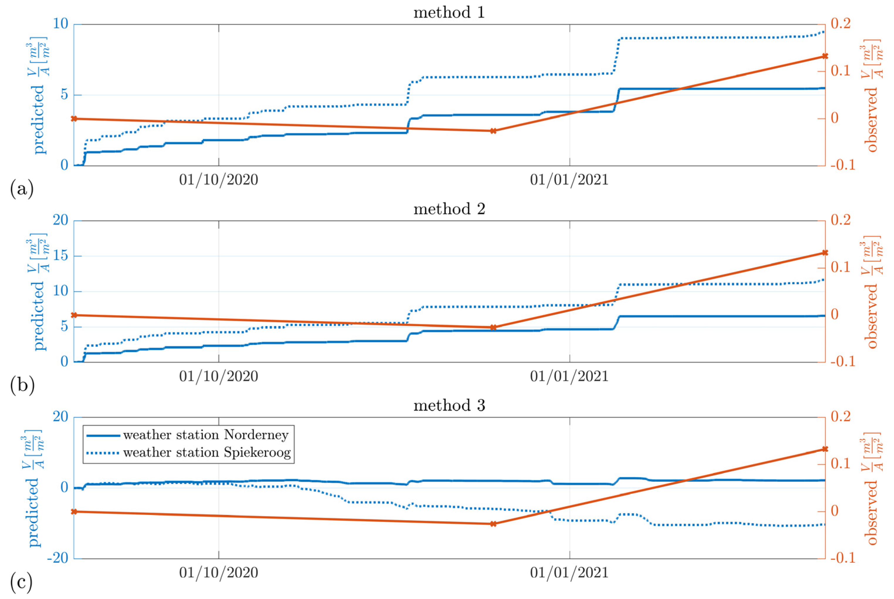
6.2. Correlation between Dune Volume Changes and Potential Aeolian Sediment Transport

Coastal dune growth is significantly related to potential aeolian sediment transport [5,6,7]. Studies of coastal dune development typically focus on measuring short-term transport processes at timescales of hours to days [5,36,61,87]. These studies often show good results between predicted and observed potential aeolian sediment transport [21,36]. Coastal dune development is also commonly studied by measuring long-term topographical changes on timescales of months to years and related to sediment transport equations [7,74,88,89]. Long-term aeolian sediment transport from the beach towards the coastal dunes is generally predicted by integrating hourly meteorological data, such as wind velocity and direction from meteorological weather stations, see Section 4.4. At these timescales, results related to dune volume changes have so far been subject to significant uncertainties [5,61]. However, Keijsers et al. (2014) [89] and De Vries et al. (2016) [6] have found good correlations on annual to decadal timescales for wide beaches W > 200 m. Strypsteen (2019) [5] found dune growth primarily determined by aeolian sediment transport from the beach on a decadal timescale.

We examined the possible correlation between dune growth influenced by sand trapping fences and potential aeolian sediment transport rates on the timescale of months. As of date, it is not clear which wind directions and associated potential sediment transport contribute to dune toe growth or erosion. Therefore, it is a frequent practice to examine different possible mechanisms according to onshore and cross-shore wind directions, see, e.g., Strypsteen (2019) [5]. We, therefore, present three different methods, which differ in whether erosion or accumulation of sand is favoured depending on the wind direction:

• Method 1: Cross-shore onshore aeolian sediment transport rates, see Equation (4), are solely used to explain coastal dune toe growth.
• Method 2: Cross-shore onshore and longshore aeolian sediment transport rates, see Equations (4) and (5), are used to calculate coastal dune toe growth.
• Method 3: Onshore wind conditions initiate dune toe growth, whereas all wind directions offshore lead to dune erosion.

In Figure 21 and Figure 22, these methods are applied for the study sites Langeoog and Norderney, respectively. A positive trend means dune volume growth; a negative trend means dune volume erosion. The blue line represents the dune volume changes based on the weather station Norderney and the dotted blue line based on the weather station Spiekeroog over the measuring time interval. In the following section, only the measurement results of the wind station Norderney are described in more detail since these correspond better with the measured values. Furthermore, Spiekeroog’s results are a multiple of Norderney’s results. The orange line indicates the observed dune volume changes derived in Section 5.1. Over the whole measuring time, there was no storm surge measured by Federal Maritime and Hydrographic Agency [90], reaching the dune toe level suggesting that aeolian processes solely and sand trapping caused a change in dune volume.

It is clearly visible that method 1 and method 2 show similar and good results in predicting the trend of the dune toe volume change for the study site Langeoog, whereas method 1 shows even better results.

Over the measured time interval, a total dune volume change of V/A_method1 = 5.3 m³/m² for method 1, V/A_method2 = 9.5 m³/m² for method 2, and of V/A_method3 = 3.7 m³/m² for method 3 was predicted.

For method 1 the average dune growth is approximately 20% of the potential aeolian sediment, whereas for method 2 approximately 10% of the potential aeolian sediment is deposited. Time intervals of a positive dune toe volume change for the predicted model agree well with areas of dune growth in the observed model. Obviously, and as can be clearly seen in Figure 21, the dune volume change is not equal to the potential sediment transport, assuming that all sediment accumulates at the sand trapping fence. Either not all sediment that is potentially transported by onshore winds to the dune toe is sedimented, and the potential sediment transport is overestimated due to the necessary simplifications made in its calculation, especially neglecting shells, sand moisture, and salt crusts.

Method 3 would suggest erosion and a decrease in dune volume. However, this erosion is most likely prevented by the sand trapping fences and a sheltering effect of the dunes landward of the dune toe.

For Norderney, the results have no significant correlation between predicted and measured values for the whole duration of the measurements. However, the final state again corresponds to the trend of volume change for method 1 and method 2. It should, however, be noted that only three measuring points are available. The growing pattern of coastal dunes following a sigmoid growth curve ([12,77]) may also explain why, for Norderney, the observed volume changes do not correlate to potential aeolian sediment transport since the growth of coastal dunes is a product of both potential transport and sand trapping.

In general, the assumption can be made that with a sufficiently long measurement period and many measurements of dune volumes, the cross-shore aeolian sediment transport rates (method 1) and additionally longshore sediment transport rates (method 2) are an appropriate approach to predicted the dune volume changes at sand trapping fences, especially for incipient coastal dune growth.

7. Conclusions and Outlook

This study provided the insights into monitoring coastal dune toe growth around and in between individual lines of brushwood of a sand trapping fence with different configurations. This work presented the results of field experiments conducted on the East Frisian islands Langeoog and Norderney, analyzing topographical changes at the dune toe influenced by a sand trapping fence as time passes. The following conclusions can be drawn from the results presented in this work:

• It is clearly visible that a particularly large amount of sand accumulated at the individual lines of brushwood of the sand trapping fence.
• In exposed fields of newly constructed sand trapping fences with potentially higher sediment supply from the beach, brushwood lines can trap more sand than in fields in the center of the sand trapping fence.
• The brushwood lines arranged parallel to the coastal dunes with a higher porosity have allowed for growth further towards the coastal dunes. For those with lower porosity, growth has been greatly increased directly at the brushwood lines.
• The orthogonally arranged deflectors at the dune toe can favour an accretion of sand at the dune toe.
• The dune growth potential at the sand trapping fence is greatest shortly after construction of the sand trapping fence and declines over time.
• The growing pattern of coastal dunes follows a sigmoid growth function with a more established coastal dune on Norderney than on Langeoog.
• For the sand trapping fence that has been in place longer, the protruding branch height and the porosity of the remaining branches seem to play a minor role for trapping sediment.
• The prevailing boundary conditions like sediment supply as well as the height and the porosity of the brushwood bundles strongly influencing the effectiveness of the different sand trapping configurations.
• In general, with a sufficiently long measurement period and number of measurements of topographical changes, the calculations of the cross-shore aeolian sediment transport rates according to method 1, or also considering longshore sediment transport rates according to method 2, is an appropriate approach to predict the trend in dune toe volume changes at sand trapping fences, especially for incipient dune formation.
• The dune toe growth of coastal dunes influenced by sand trapping fences is a product of both potential transport and sand trapping.

Repeated UAV surveys provide an accurate method to study detailed changes in dune toe volume on a timescale of months to years. We strongly recommend extending the knowledge of the influence of sand trapping fences on aeolian sediment transport and dune toe development in standardized wind tunnel experiments to gain quantitative data.

References

1. Kystdirektoratet. Aeolian Sediment Transport and Natural Dune Development, Skodbjerge, Denmark, Skodbjerge, Denmark. Lemvig.: Interreg. North Sea Region. Building with Nature. 2020. Available online: https://northsearegion.eu/media/12719/aeolian-sediment-transport-and-natural-dune-development-skodbjerge-denmark.pdf (accessed on 21 June 2021).
2. Generalplan Küstenschutz Niedersachsen: Ostfriesische Inseln, Küstenschutz Band 2.; Niedersächsischer Landesbetrieb für Wasserwirtschaft, Küsten- und Naturschutz (Lower Saxony Water Management, Coastal Protection and Nature Conversation Agency), Ed. 2010. Available online: https://www.nlwkn.niedersachsen.de/startseite/hochwasser_kustenschutz/kustenschutz/generalplane_fur_insel_und_kustenschutz/generalplan-kuestenschutz-45183.html (accessed on 21 June 2021).
3. Peters, K.; Pohl, M. Kuratorium für Forschung im Küsteningenieurwesen (German Coastal Engineering Research Council). Die Küste (The Coast), Issue 88, EAK 2020. Empfehlungen für die Ausführung von Küstenschutzwerken durch den Ausschuss für Küstenschutzwerke der Deutschen Gesellschaft für Geotechnik e.V. und der Hafenbautechnischen Gesellschaft e.V. (Recommendations for Coastal Protection Structures. Working Group ’Coastal Protection Structures’ as a Joint Commitee of the German Port Geotechnical Society and the German Port Technology Association), 3rd ed.; Westholsteinische Verlagsanstalt Boyens & Co.: Heide, Germany, 2020. [Google Scholar]
4. Hesp, P. Foredunes and blowouts: Initiation, geomorphology and dynamics. Geomorphology 2002, 48, 245–268. [Google Scholar] [CrossRef]
5. Strypsteen, G. Monitoring and Modelling Aeolian Sand Transport at the Belgian Coast. Ph.D. Thesis, KU LEUVEN, Brugge, Belgium, 2019. [Google Scholar]
6. De Vries, S.; Southgate, H.N.; Kanning, W.; Ranasinghe, R. Dune behavior and aeolian transport on decadal timescales. Coast. Eng. 2012, 67, 41–53. [Google Scholar] [CrossRef]
7. Bagnold, R.A. The Physics of Blown Sand and Desert Dunes; Springer: Dordrecht, The Netherlands, 1941. [Google Scholar]
8. Van Thiel de Vries, J.S.M. Dune Erosion during Storm Surges. Ph.D. Thesis, Technische Universität Delft, Amsterdam, The Netherlands, 2009. [Google Scholar]
9. Staudt, F.; Gijsman, R.; Ganal, C.; Mielck, F.; Wolbring, J.; Hass, H.C.; Goseberg, N.; Schüttrumpf, H.; Schlurmann, T.; Schimmels, S. The sustainability of beach nourishments: A review of nourishment and environmental monitoring practice. J. Coast Conserv. 2021, 25. [Google Scholar] [CrossRef]
10. Martínez, M.L.; Hesp, P.A.; Gallego-Fernández, J.B. (Eds.) Coastal Dune Restoration: Trends and Perspectives. In Restoration of Coastal Dunes; Springer: Berlin/Heidelberg, Germany, 2013; pp. 323–339. ISBN 978-3-642-33444-3. [Google Scholar]
11. Hanley, M.E.; Hoggart, S.; Simmonds, D.J.; Bichot, A.; Colangelo, M.A.; Bozzeda, F.; Heurtefeux, H.; Ondiviela, B.; Ostrowski, R.; Recio, M.; et al. Shifting sands? Coastal protection by sand banks, beaches and dunes. Coast. Eng. 2014, 87, 136–146. [Google Scholar] [CrossRef]
12. Dalyander, P.S.; Mickey, R.C.; Passeri, D.L.; Plant, N.G. Development and Application of an Empirical Dune Growth Model for Evaluating Barrier Island Recovery from Storms. J. Mar. Sci. Eng. 2020, 8, 977. [Google Scholar] [CrossRef]
13. Galiforni Silva, F. Beach-Dune Systems Near Inlets: Linking Subtidal and Subaerial Morphodynamics. Ph.D. Thesis, University of Twente, Enschede, The Netherlands, 2019. [Google Scholar]
14. Short, A.D.; Hesp, P.A. Wave, Beach and Dune Interactions in Southeastern Australia. Mar. Geol. 1982, 259–284. [Google Scholar] [CrossRef]
15. Arens, S.M. Rates of aeolian transport on a beach in a temperate humid climate. Geomorphology 1996, 17, 3–18. [Google Scholar] [CrossRef] [Green Version]
16. Van Rijn, L.C. Coastal erosion and control. Ocean Coast. Manag. 2011, 54, 867–887. [Google Scholar] [CrossRef]
17. D’Alessandro, F.; Tomasicchio, G.R. Wave–dune interaction and beach resilience in large-scale physical model tests. Coast. Eng. 2016, 116, 15–25. [Google Scholar] [CrossRef]
18. Schweiger, C.; Kaehler, C.; Koldrack, N.; Schuettrumpf, H. Spatial and temporal evaluation of storm-induced erosion modelling based on a two-dimensional field case including an artificial unvegetated research dune. Coast. Eng. 2020, 161, 103752. [Google Scholar] [CrossRef]
19. Sutton-Grier, A.; Gittman, R.; Arkema, K.; Bennett, R.; Benoit, J.; Blitch, S.; Burks-Copes, K.; Colden, A.; Dausman, A.; DeAngelis, B.; et al. Investing in Natural and Nature-Based Infrastructure: Building Better Along Our Coasts. Sustainability 2018, 10, 523. [Google Scholar] [CrossRef] [Green Version]
20. Baas, A.C.W.; Sherman, D.J. Spatiotemporal Variability of Aeolian Sand Transport in a Coastal Dune Environment. J. Coast. Res. 2006, 225, 1198–1205. [Google Scholar] [CrossRef]
21. Van Rijn, L.C.; Strypsteen, G. A fully predictive model for aeolian sand transport. Coast. Eng. 2019, 156. [Google Scholar] [CrossRef]
22. Sherman, D.J.; Li, B.; Ellis, J.T.; Farrell, E.J.; Maia, L.P.; Granja, H. Recalibrating aeolian sand transport models. Earth Surf. Process. Landf. 2013, 38, 169–178. [Google Scholar] [CrossRef]
23. Grafals-Soto, R. Understanding the Effetcs of Sand Fence Usage and the Resulting Landscape, Landforms and Vegetation Patterns: A New Jersey Example. Ph.D. Thesis, University of New Brunswick, New Brunswick, NJ, USA, 2010. [Google Scholar]
24. Grafals-Soto, R.; Nordstrom, K. Sand fences in the coastal zone: Intended and unintended effects. Environ. Manag. 2009, 44, 420–429. [Google Scholar] [CrossRef] [PubMed]
25. Li, B.; Sherman, D.J. Aerodynamics and morphodynamics of sand fences: A review. Aeolian Res. 2015, 17, 33–48. [Google Scholar] [CrossRef]
26. Zhang, N.; Kang, J.-H.; Lee, S.-J. Wind tunnel observation on the effect of a porous wind fence on shelter of saltating sand particles. Geomorphology 2010, 120, 224–232. [Google Scholar] [CrossRef]
27. Dong, Z.; Luo, W.; Qian, G.; Wang, H. A wind tunnel simulation of the mean velocity fields behind upright porous fences. Agric. For. Meteorol. 2007, 146, 82–93. [Google Scholar] [CrossRef]
28. Dong, Z.; Chen, G.; He, X.; Han, Z.; Wang, X. Controlling blown sand along the highway crossing the Taklimakan Desert. J. Arid Environ. 2004, 57, 329–344. [Google Scholar] [CrossRef]
29. Hotta, S.; Horikawa, K. Function of Sand Fence Placed in Front of Embankment. In Proceedings of the 22nd Conference on Coastal Engineering 2–6 July 1990, Delft, The Netherlands, 2–6 July 1990; pp. 2754–2767. [Google Scholar] [CrossRef]
30. Adriani, M.J.; Terwindt, J.H.J. Sand Stabilization and Dune Building; Government Publishing Office: Hague, The Netherlands, 1974; ISBN 9012004985.
31. Ning, Q.; Li, B.; Ellis, J.T. Fence height control on sand trapping. Aeolian Res. 2020, 46, 100617. [Google Scholar] [CrossRef]
32. Yu, Y.; Zhang, K.; An, Z.; Wang, T.; Hu, F. The blocking effect of the sand fences quantified using wind tunnel simulations. J. Mt. Sci. 2020, 17, 2485–2496. [Google Scholar] [CrossRef]
33. Lima, I.A.; Araújo, A.D.; Parteli, E.J.R.; Andrade, J.S., Jr.; Herrmann, H.J. Optimal Array of Sand Fences; 2017. Available online: http://arxiv.org/pdf/1702.05114v1 (accessed on 21 June 2021).
34. Anthony, E.J.; Vanhee, S.; Ruz, M.-H. An assessment of the impact of experimental brushwood fences on foredune sand accumulation based on digital elelvation models. Ecol. Eng. 2007, 31, 41–46. [Google Scholar] [CrossRef]
35. Ruz, M.-H.; Anthony, E.J. Sand trapping by brushwood fences on a beach-foredune contact: The primacy of the local sediment budget. Zeitschrift für Geomorphologie 2008, 52, 179–194. [Google Scholar] [CrossRef]
36. Eichmanns, C.; Schüttrumpf, H. Investigating Changes in Aeolian Sediment Transport at Coastal Dunes and Sand Trapping Fences: A Field Study on the German Coast. JMSE 2020, 8, 1012. [Google Scholar] [CrossRef]
37. Sanromualdo-Collado, A.; Hernández-Cordero, A.I.; Viera-Pérez, M.; Gallego-Fernández, J.B.; Hernández-Calvento, L. Coastal Dune Restoration in El Inglés Beach (Gran Canaria, Spain): A Trial Study. REA 2021, 187–204. [Google Scholar] [CrossRef]
38. Gerhardt, P. Im Auftrage des Kgl. Preuss. In Handbuch des Deutschen Dünenbaues; Johannes, A., Paul, B., Alfred, J., Eds.; Verlagsbuchhandlung Paul Parey: Berlin, Germany, 1990. [Google Scholar]
39. Reise, K. Coast of change: Habitat loss and transformations in the Wadden Sea. Helgol. Mar. Res. 2005, 59, 9–21. [Google Scholar] [CrossRef]
40. De Groot, A.V.; Oost, A.P.; Veeneklaas, R.M.; Lammerts, E.J.; van Duin, W.E.; van Wesenbeeck, B.K. Tales of island tails: Biogeomorphic development and management of barrier islands. J. Coast Conserv. 2017, 21, 409–419. [Google Scholar] [CrossRef] [Green Version]
41. Hillmann, S.; Blum, H.; Thorenz, F. National Analysis—Germany Lower Saxony.: Niedersächsischer Landesbetrieb für Wasserwirtschaft, Küsten und Naturschutz (Lower Saxony Water Management, Coastal Protection and Nature Conservation Agency); NLWKN: Lower Saxony, Germany, 2019. [Google Scholar]
42. Federal Agency for Cartography and Geodesy. Geodaten der Deutschen Landesvermessung. Bundesamt für Kartographie und Geodäsie (Federal Agency for Cartography and Geodesy); Federal Agency for Cartography and Geodesy: Leipzig, Germany; Available online: http://sg.geodatenzentrum.de/web_public/nutzungsbedingungen.pdf (accessed on 29 March 2021).
43. Bundesamt für Schifffahrt und Hydrographie. Gezeitenkalender 2021: Hoch- und Niedrigwasserzeiten für die Deutsche Bucht und deren Flussgebiete; Bundesamt für Schifffahrt und Hydrographie: Hamburg, Germany, 2020. [Google Scholar]
44. Thorenz, F.; Kuratorium für Forschung im Küsteningenieurwesen (German Coastal Engineering Research Council). Die Küste (The Coast), Issue 74, EAK; Coastal Flood Defence and Coastal Protection along the North Sea Coast of Niedersachsen; Kuratorium für Forschung im Küsteningenieurwesen (German Coastal Engineering Research Council): Hamburg, Germany, 2008. [Google Scholar]
45. Hayes, M.O. Barrier Island Morphology as a Function of Tidal and Wave regime: Barrier Islands from the Gulf of St. Lawrence to the Gulf of Mexic; Academic Press: New York, NY, USA, 1979; pp. 1–27. [Google Scholar]
46. Niemeyer, H.D. Long Term Morphodynamical Development of the East Frisian Island and Coast. In Proceedings of the 24th International Conference on Coastal Engineering, Kobe, Japan, 23–28 October 1994. [Google Scholar]
47. Hagen, R.; Freund, J.; Plüß, A.; Ihde, R. (Eds.) Validierungsdokument EasyGSH-DB Nordseemodell. Teil: UnTRIM2–SediMorph–UnK; Federal Waterways Engineering and Research Institute: Karlsruhe, Germany, 2019. [Google Scholar]
48. DWD. Climate Data Center. 2021. Available online: https://cdc.dwd.de/portal/ (accessed on 1 April 2021).
49. Ladage, F. Vorarbeiten zu Schutzkonzepten für die Ostfriesischen Inseln—Morphologische Entwicklung um Langeoog im Hinblick auf die verstärkten Dünenabbrüche vor dem Pirolatal; NLWKN: Norderney, Germany, 2002. [Google Scholar]
50. Donker, J.; van Maarseveen, M.; Ruessink, G. Spatio-Temporal Variations in Foredune Dynamics Determined with Mobile Laser Scanning. JMSE 2018, 6, 126. [Google Scholar] [CrossRef] [Green Version]
51. Lower Saxony Water Management, Coastal Protection and Nature Conversation Agency. Documentation of the Configuration of the Installed Sand Trapping Fences on Langeoog and Norderney; Lower Saxony Water Management, Coastal Protection and Nature Conversation Agency: Hannover, Germany, 2020. [Google Scholar]
52. MATLAB, Version 9.510.944444 (R2018b); The MathWorks Inc.: Natick, MA, USA, 2018.
53. Azzeh, J.; Zahran, B.; Alqadi, Z. Salt and Pepper Noise: Effects and Removal. Int. J. Inform. Vis. 2018, 2, 252. [Google Scholar] [CrossRef] [Green Version]
54. Image Analyst. Image Segmentation Tutorial Image Analyst (2021). Image Segmentation Tutorial. MATLAB Central File Exchange 2021. Available online: https://www.mathworks.com/matlabcentral/fileexchange/25157-image-segmentation-tutorial (accessed on 21 June 2021).
55. DJI. Phantom 4 RTK: Product Specifications. Available online: https://www.dji.com/de/phantom-4-rtk/info (accessed on 31 March 2021).
56. Javad. JAVAD Global Navigation Satellite System (GNSS) Receiver SigmaD-G3D: Data Sheet GNSS Receiver Sigma-3. Available online: http://download.javad.com/manuals/ (accessed on 31 March 2021).
57. AgiSoft Metashape Professional. Version 1.6.5 Build 11249, 64 Bit; AgiSoft Metashape Professional: St. Petersburg, Russia, 2020; Available online: https://www.agisoft.com/downloads/installer/ (accessed on 27 July 2021).
58. ESRI ArcGIS Desktop. Version 10.5.1, 64 Bit. ESRI: 2017. Available online: https://www.esri.com/en-us/arcgis/products/arcgis-pro/overview/ (accessed on 27 July 2021).
59. Van Rijn, L.C. Aeolian Transport over a Flat Sediment Surface. Aeolian Transp. 2019. Available online: www.leovanrijn-sediment.com (accessed on 27 July 2021).
60. Nickling, W.G.; McKenna Neumann, C. (Eds.) Aeolian Sediment Transport, 2nd ed.; Springer: Dordrecht, The Netherlands, 2009; ISBN 978-1-4020-5718-2. [Google Scholar]
61. Sarre, R.D. Aeolian sand drift from the intertidal zone on a temperate beach: Potential and actual rates. Earth Surf. Process. Landf. 1989, 14, 247–258. [Google Scholar] [CrossRef]
62. De Vries, S. Physics of Blown Sand and Coastal Dunes; Delft University of Technology: Delft, The Netherlands, 2013. [Google Scholar]
63. Dong, Z.; Liu, X.; Wang, H.; Wang, X. Aeolian sand transport: A wind tunnel model. Sediment. Geol. 2003, 161, 71–83. [Google Scholar] [CrossRef]
64. Davidson-Arnott, R.; Yang, Y.; Ollerhead, J.; Hesp, P.; Walker, I.J. The effects of surface moisture on aeolian sediment transport threshold and mass flux on a beach. Earth Surf. Process. Landf. 2007, 33, 55–74. [Google Scholar] [CrossRef]
65. Delgado-Fernandez, I. A review of the application of the fetch effect to modelling sand supply to coastal foredunes. Aeolian Res. 2010, 2, 61–70. [Google Scholar] [CrossRef] [Green Version]
66. Hoonhout, B.; de Vries, S. Field measurements on spatial variations in aeolian sediment availability at the Sand Motor mega nourishment. Aeolian Res. 2016, 24, 93–104. [Google Scholar] [CrossRef] [Green Version]
67. Bauer, B.O.; Davidson-Arnott, R.; Hesp, P.A.; Namikas, S.L.; Ollerhead, J.; Walker, I.J. Aeolian sediment transport on a beach: Surface moisture, wind fetch, and mean transport. Geomorphology 2009, 105, 106–116. [Google Scholar] [CrossRef]
68. Bauer, B.O.; Davidson-Arnott, R.G. A general framework for modeling sediment supply to coastal dunes including wind angle, beach geometry, and fetch effects. Geomorphology 2003, 49, 89–108. [Google Scholar] [CrossRef]
69. Lynch, K.; Jackson, D.W.T.; Cooper, J.A.G. Aeolian fetch distance and secondary airflow effects: The influence of micro-scale variables on meso-scale foredune development. Earth Surf. Process. Landforms 2008, 33, 991–1005. [Google Scholar] [CrossRef]
70. Davidson-Arnott, R.G.; MacQuarrie, K.; Aagaard, T. The effect of wind gusts, moisture content and fetch length on sand transport on a beach. Geomorphology 2005, 68, 115–129. [Google Scholar] [CrossRef]
71. Spies, P.-J.; McEwan, I.K. Equilibration of saltation. Earth Surf. Process. Landf. 2000, 25, 437–453. [Google Scholar] [CrossRef]
72. Davidson-Arnott, R.; Law, M.N. Measurement and Prediction of Long-Term Sediment Supply to Coastal Foredunes. J. Coast. Res. 1996, 12, 654–663. [Google Scholar]
73. Field, J.P.; Pelletier, J.D. Controls on the aerodynamic roughness length and the grain-size dependence of aeolian sediment transport. Earth Surf. Process. Landf. 2018, 43, 2616–2626. [Google Scholar] [CrossRef]
74. Hsu, S.A. Computing Eolian sand Transport from routine weather data. In Proceedings of the 14th Conference on Coastal Engineering, Copenhagen, Denmark, 24–28 June 1974; pp. 1619–1626. [Google Scholar] [CrossRef]
75. Shao, Y.; Lu, H. A simple expression for wind erosion threshold friction velocity. J. Geophys. Res. 2000, 105, 22437–22443. [Google Scholar] [CrossRef]
76. Nickling, W.G.; Davidson-Arnott, R. (Eds.) Aeolian Sediment Transport on Beaches and Coastal Sand Dunes; Canadian Coastal Science and Engineering Association: Guelph, ON, Canada, 1990. [Google Scholar]
77. Houser, C.; Wernette, P.; Rentschlar, E.; Jones, H.; Hammond, B.; Trimble, S. Post-storm beach and dune recovery: Implications for barrier island resilience. Geomorphology 2015, 234, 54–63. [Google Scholar] [CrossRef]
78. Keijsers, J.; de Groot, A.V.; Riksen, M. Vegetation and sedimentation on coastal foredunes. Geomorphology 2015, 228, 723–734. [Google Scholar] [CrossRef]
79. Miri, A.; Dragovich, D.; Dong, Z. Wind-borne sand mass flux in vegetated surfaces—Wind tunnel experiments with live plants. CATENA 2019, 172, 421–434. [Google Scholar] [CrossRef]
80. Cohn, N.; Hoonhout, B.; Goldstein, E.; de Vries, S.; Moore, L.; Durán Vinent, O.; Ruggiero, P. Exploring Marine and Aeolian Controls on Coastal Foredune Growth Using a Coupled Numerical Model. JMSE 2019, 7, 13. [Google Scholar] [CrossRef] [Green Version]
81. Hacker, S.D.; Zarnetske, P.; Seabloom, E.; Ruggiero, P.; Mull, J.; Gerrity, S.; Jones, C. Subtle differences in two non-native congeneric beach grasses significantly affect their colonization, spread, and impact. Oikos 2012, 121, 138–148. [Google Scholar] [CrossRef]
82. Durán, O. Vegetated Dunes and Barchan Dune Fields. Ph.D. Thesis, Universität Stuttgart, Stuttgart, Germany, 2007. [Google Scholar]
83. Durán, O.; Moore, L.J. Vegetation controls on the maximum size of coastal dunes. Proc. Natl. Acad. Sci. USA 2013, 110, 17217–17222. [Google Scholar] [CrossRef] [Green Version]
84. Arens, S.M.; Baas, A.C.W.; Van Boxel, J.H.; Kalkman, C. Influence of reed stem density on foredune development. Earth Surf. Process. Landf. 2001, 26, 1161–1176. [Google Scholar] [CrossRef]
85. Van der Wal, D. Effects of fetch and surface texture on aeolian sand transport on two nourished beaches. J. Arid Environ. 1998, 39, 533–547. [Google Scholar] [CrossRef]
86. Jackson, N.L.; Nordstrom, K.F. Aeolian sediment transport and landforms in managed coastal systems: A review. Aeolian Res. 2011, 3, 181–196. [Google Scholar] [CrossRef]
87. Jackson, N.L.; Nordstrom, K.F. Aeolian transport of sediment on a beach during and after rainfall, Wildwood, NJ, USA. Geomorphology 1997. [Google Scholar] [CrossRef]
88. Delgado-Fernandez, I. Meso-scale modelling of aeolian sediment input to coastal dunes. Geomorphology 2011, 130, 230–243. [Google Scholar] [CrossRef] [Green Version]
89. Keijsers, J.G.S.; Poortinga, A.; Riksen, M.J.P.M.; Maroulis, J. Spatio-temporal variability in accretion and erosion of coastal foredunes in the Netherlands: Regional climate and local topography. PLoS ONE 2014, 9, e91115. [Google Scholar] [CrossRef] [Green Version]
90. Bundesamt für Schifffahrt und Hydrographie. Berichte zu Sturmfluten und extremen Wasserständen: Nordsee; Bundesamt für Schifffahrt und Hydrographie: Hamburg, Germany, 2021. [Google Scholar]
Figure 1. (a) Aerial drone photograph of the sand trapping fence consisting of brushwood on the study site of Norderney and (b) a close-up of the sand trapping fence seen from the coastal dunes, showing sand being trapped in between the brushwood lines (9 March 2021).
Jmse 09 00850 g001
Figure 2. (a) Location of the East Frisian Islands along the North Sea coast in Germany, (b) showing the East Frisian Islands, (c) study site Langeoog, and (d) study site Norderney (with permission from © GeoBasis-DE/ BKG, 2021 [42], data obtained from [2,42]).
Jmse 09 00850 g002
Figure 3. Hourly averaged wind velocities and wind directions from the weather station (a) Norderney and (b) Spiekeroog from 1 May 2020 to 31 March 2021 (wind data obtained from [48]).
Jmse 09 00850 g003
Figure 4. Aerial photograph of the sand trapping fence at the study site of Langeoog showing the four different configurations differing in their arrangement of brushwood lines parallel and orthogonal to the coastal dunes and the number of bundles of brushwood per running meter n [bb/m] and their porosity ε [%], respectively. The red polygons delimit fields 1–22, the fields west and east, and a green polygon the reference field.
Jmse 09 00850 g004
Figure 5. Aerial photograph of the sand trapping fence at the study site of Norderney showing the four different configurations differing in their arrangement of brushwood lines parallel and orthogonal to the coastal dunes and the number of bundles of brushwood per running meter n [bb/m] and their porosity ε [%], respectively. The red polygons delimit fields 1–22, the fields west and east, and a green polygon the reference field.
Jmse 09 00850 g005
Figure 6. (a) Standardized section of the sand trapping fence with 5 bb/m, (b) standardized section of the sand trapping fence with 3–4 bb/m, (c) standardized section of the sand trapping fence with 2 bb/m.
Jmse 09 00850 g006
Figure 7. Result of image processing to determine the sand trapping fence’s porosity with (a) the masked image, (b) the binary image, and (c) the noise cleared image of the standardized section (configuration 2*) of the sand trapping fence on Norderney with n = 3–4 bb/m.
Jmse 09 00850 g007
Figure 8. Schematic sketch of the coastal beach-dune system (adapted from [5]).
Jmse 09 00850 g008
Figure 9. Orientation of the coastline of (a) the study site of Langeoog and (b) Norderney. Green arrows show the onshore directions of aeolian sediment transport towards the coastal dunes, the angles O [°] show the wind direction (concerning the north), and ddj [°] the angles between the coastal orientation and the wind direction (methodology adapted from [5]).
Jmse 09 00850 g009
Figure 10. (a) Orthophotograph with digital elevation heights from 3 to 8 mNHN of study site Langeoog on 20 May 2020, (b) on 15 June 2020, (c) on 27 August 2020, (d) Orthophotograph with digital elevation heights from 3 to 8 mNHN of study site Langeoog on 26 October 2020, (e) on 14 December 2020, (f) on 12 March 2021.
Jmse 09 00850 g010aJmse 09 00850 g010b
Figure 11. Differences in elevation heights derived from the DEM of study site Langeoog between 20 May 2020 and 12 March 2021.
Jmse 09 00850 g011
Figure 12. (ad) Dune volume changes per area V/A [m³/m²] over time for the different sand trapping configurations as well as (e) the most westward and the most eastward fields. (f) Reference field on the study site Langeoog.
Jmse 09 00850 g012
Figure 13. (a) Orthophotograph with digital elevation heights from 3–8 mNHN of study site Norderney on 24 August 2020, and on (b) 12 December 2020, (c) Orthophotograph with digital elevation heights from 3–8 mNHN of study site Norderney on 9 March 2021.
Jmse 09 00850 g013aJmse 09 00850 g013b
Figure 14. Differences in elevation heights derived from the DEM of study site Norderney between 24 August 2020 and 09 March 2021.
Jmse 09 00850 g014
Figure 15. (ad) Dune volume changes per area V/A [m³/m²] over time for the different sand trapping configuration as well as (e) the most westward and the most eastward fields. (f) Reference field on the study site Norderney.
Jmse 09 00850 g015
Figure 16. (a) Longshore profiles onshore and (b) offshore of the sand trapping fence of the study site Langeoog on 20 May 2020, 15 June 2020, 27 August 2020, 26 October 2020, 14 December 2020, and 12 March 2021. The dashed lines divide the study site into individual configurations.
Jmse 09 00850 g016
Figure 17. (a) Longshore profiles onshore, (b) between parallel brushwood lines, and (c) offshore of study site Norderney on 24 August 2020, 12 December 2020, and 09 March 2021. The dashed lines divide the study site into individual configurations.
Jmse 09 00850 g017
Figure 18. Cross-shore dune profiles of (a) config. 1, (b) config. 2, (c) config. 3, and (d) config. 4 of study site Langeoog on 20 May 2020, 15 June 2020, 27 August 2020, 26 October 2020, 14 December 2020, and 12 March 2021.
Jmse 09 00850 g018
Figure 19. Cross-shore dune profiles of (a) config. 1, (b) config. 2, (c) config. 3, and (d) config. 4 of study Norderney on 24 August 2020, 12 December 2020, and 09 March 2021.
Jmse 09 00850 g019
Figure 20. Sand volume changes from August 2020 to March 2021 (197 days) of different sand trapping configurations on Langeoog (darker colors) and Norderney (brighter colors) presented as a boxplot based on (a) their average porosity ε ¯ [%] and (b) their configuration type 1 (blue), type 2 (orange), type 3 (green), and type 4 (purple).
Jmse 09 00850 g020
Figure 21. Predicted dune volume changes based on the transportation Equation (4) and Equation (5) obtained by the wind data from weather station Norderney (blue line) and Spiekeroog (dotted blue line), and observed dune volume changes (orange line) for study site Langeoog applying (a) method 1, (b) method (2), and (c) method (3).
Jmse 09 00850 g021
Figure 22. Predicted dune volume changes based on the transportation Equation (4) and Equation (5) obtained by the wind data from weather station Norderney (blue line) and Spiekeroog (dotted blue line), and observed dune volume changes (orange line) for study site Norderney applying (a) method 1, (b) method (2), and (c) method (3).
Jmse 09 00850 g022