Dynamics and Transformation of Sea Surface Gravity Waves at the Shelf of Decreasing Depth

Abstract

This paper reviews the results of the processing of synchronized data on hydrosphere pressure variations and the Earth’s crust deformation in the microseismic range (5–15 s), obtained over the course of numerous experiments, using a coastal laser strainmeter and laser meters of hydrosphere pressure variations installed in various points of the Sea of Japan shelf. Interpreting the results, we have discovered new regularities in the dynamics of surface progressive gravity waves, and their transformation into primary microseisms, when waves move at the shelf of decreasing depth. For example, we found non-isochronous behavior of progressive waves, which manifests itself in a decrease in the periods of gravity waves due to the transformation of a part of their energy into the energy of primary microseisms. Furthermore, when processing the synchronous fragments of the records, made by laser strainmeters and laser meters of hydrosphere pressure variations, we identified approximate zones of the most effective transformation of the energy of gravity progressive waves into the energy of primary microseisms, which start from the depth of less than a half-wavelength and stretch to the surf zone.

1. Introduction

Many works are devoted to the process of the emergence and development of sea progressive and standing surface gravity waves. We do not discuss it in this paper, but let us only note that the main parameters of emerging sea gravity waves depend on wind speed and the time of its activity over a particular water area, acceleration magnitudes, geometric characteristics of the water areas, natural conditions that generate head waves with the period, close to the period of an incident sea gravity wave. Interesting are the issues associated with dynamics of surface gravity waves during their movement at the shelf of decreasing depth and their transformation into primary microseisms. When moving at the shelf, these waves, especially at depths of less than a half-length of a sea gravity wave, are subject to various changes, associated primarily with the impact of nonlinear and dissipative processes. Modern theoretical and experimental studies show that nonlinear processes are dominant, both in deep and shallow water.

Of particular interest is the issue of the transformation of the spectra of gravity waves as they propagate at the shelf of decreasing depth. In this case, the main maximum can shift to both the high-frequency and low-frequency spectral regions. For example, [1] presents the results of experimental and model studies of the evolution of frequency spectra for groups of dispersive focusing waves in a two-dimensional wave reservoir. It shows that there is a nonlinear energy transfer to low-frequency spectral components, which cannot be detected easily. The energy dissipation in the spectral maximum region is ascertained, which increases the energy in the higher-frequency range, which depends on the Benjamin–Feir index. It is demonstrated that the energy increase in the low-frequency range occurs, at least partly, due to nonlinear energy transfer before a wave breaks, and that breaking of a wave cannot necessarily increase the energy in this range.

As stated in [2], the waves covering a long distance over a very gradually sloping bottom undergo more nonlinear evolution than the waves coming over a steeply sloping bottom, so the peculiarities of the waves’ nonlinearity depend on propagation distance and water depth. In particular, additional frequency peaks can be formed due to spectrum broadening as a result of backward energy transfer from higher frequencies [3] and from lower (infragravity) frequencies to the main peak [4]. The mechanisms of energy transfer between spectral peaks of sea gravity waves in the frequency range of 0.05–0.5 Hz are considered. These energy transfers occur among the three phase-coupled frequencies and are called nonlinear triadic interactions. The summarized interactions transfer energy from the main spectral peak to the spectral peaks many times, which is often referred to as higher harmonics. The development of higher harmonics is associated with a skewed shape of sea waves during shallowing and an asymmetric saw-like shape during breakdown very close to the coast [5]. Simultaneously with transformation of the sea wave shape, the energy is transferred to lower frequencies of infragravity (0.005–0.05 Hz) due to difference interactions, forming bound long waves.

There are interesting results in [6,7,8]. It was demonstrated that as nonlinearity increases, the crest distribution deviates more and more from its linear analog. The general nature of this deviation is propagation of the density mass towards larger and smaller crests, which is consistent with vertically asymmetric properties of nonlinear waves, which are known to have shallower troughs and sharper and larger crests than their linear analog. Nonlinearity increases and peak period decreases due to the destructive interference of the second-order free harmonics. In [8], it is stated that variability of wave periods for waves of a given height is inversely proportional to the wave height. However, at the same time, even the influence of nonlinearities on the wave periods has not been fully studied. This requires, first of all, complex experimental field studies. The mechanism of transformation of the progressive sea surface wave energy into the energy of primary microseisms is also associated with the nonlinear transformation of sea gravity waves as they move at the shelf of decreasing depth. At the same time, the issue of the bottom sloping, required for effective transformation of this energy, has not been fully investigated. Hasselman [9] considered a constant sloping seabed and calculated the seismic response for frequencies from 0.05 to 0.1 Hz, which is known as the main microseismic band. The pressure pattern at the seabed is characterized by a wide power spectrum in the wavenumber range, and thus is equivalent to the vertical point force, by which seismic response can be estimated, e.g., [9,10]. This theory was successfully applied to slowly changing bottom slopes at seismic noise frequencies below 0.03 Hz [11]. For primary microseisms with a frequency of 0.05 < f < 0.1 Hz, Hasselman [9] used the lowest slope of 3%. Recently, Ardhuin et al. [11] showed that the primary microseismic signal, measured at the French seismic station Saint Sauveur en Rue (the geoscope network), requires an average ocean bottom slope of 6% at depths of about 20 m, while the average slopes on the French continental shelves are about 0.1% or less. It is difficult to explain such a large difference by additional effects not included in these models. Another reason why a constant or slowly changing bottom slope is not a satisfactory model for primary microseisms is that the horizontal component of the equivalent point force, equal to the vertical force multiplied by the bottom slope, is too weak to explain the observed kinetic wave energy [12,13,14].

In the presented work, when processing and analyzing the experimental data, we will consider nonlinear mechanisms of the transformation of the energy of surface gravity waves and their transformation into primary microseisms when moving at the shelf of decreasing depth.

2. Experimental Studies

The paper analyzes the results of the processing of the experimental data on hydrosphere pressure variations and the Earth’s crust deformations, obtained over the course of experimental work using laser meters of hydrosphere pressure variations and laser strainmeters. The laser strainmeters with measuring arms of 52.5 and 17.5 m are stationary, installed at Schulz Cape of Peter the Great Bay, the Sea of Japan (Russia), at the depth of 3–5 m in underground hydro- and thermally insulated rooms at coordinates 42.58° N and 131.157° E [14]. The laser strainmeters are located at about 70 m above the sea level. The optical part of each laser strainmeter is built based on the use of a modified Michelson interferometer of an unequal-arm type, using frequency-stabilized helium-neon lasers with long-term stability from 10–9 to 10–12 as a light source. The main interference unit of the Michelson interferometer of each laser strainmeter, together with the digital recording system, is located in a separate hydro- and thermally insulated room. The auxiliary interference unit of the Michelson interferometer, consisting of a corner reflector with an alignment system, is located in another hydro- and thermally insulated room. Between the main interference unit and the auxiliary interference unit, a laser beam propagates through a sealed pipeline, consisting of stainless-steel pipes, hermetically sealed at the ends by optical windows. Figure 1 shows photographs of the main interference unit of the 52.5 m laser strainmeter (Figure 1a) and an underground vacuum pipeline (Figure 1b). The measuring arms of laser strainmeters are practically orthogonal to each other and relatively positioned at the angle of 92°. The laser strainmeter with a measuring arm of 52.5 m is oriented at the angle of 18° relative to the meridian line, and the strainmeter with a measuring arm of 17.5 m is oriented at the angle of 110° relative to the same line. The main interference unit of the 52.5-meter laser strainmeter is installed on a massive concrete monolith with height of about 3 m, which is rigidly connected in the lower part to the hard rocks of Shultz Cape, consisting of compressed loam. The corner reflector of the 52.5-meter laser strainmeter is rigidly attached to a 1-meter-high concrete monolith, which is connected to a granite cliff. The described laser strainmeters have the following technical characteristics: an operating frequency range from 0 (conditionally) to 100 Hz, and measuring accuracy of the displacement of the Earth’s crust plates 0.03 nm, which can be improved through appropriate technical measures.

The laser meters of hydrosphere pressure variations [15] in their improved version were described in [16]. For several years, we installed them at various shelf points, both inside and outside Vityaz Bay, in the seaward part off Shultz Cape. At present, these laser meters of hydrosphere pressure variations have the following technical characteristics: an operating frequency range from 0 (conditionally) to 1000 Hz, a measuring accuracy of hydrosphere pressure variations 0.24 mPa, and operating depths to 50 m. 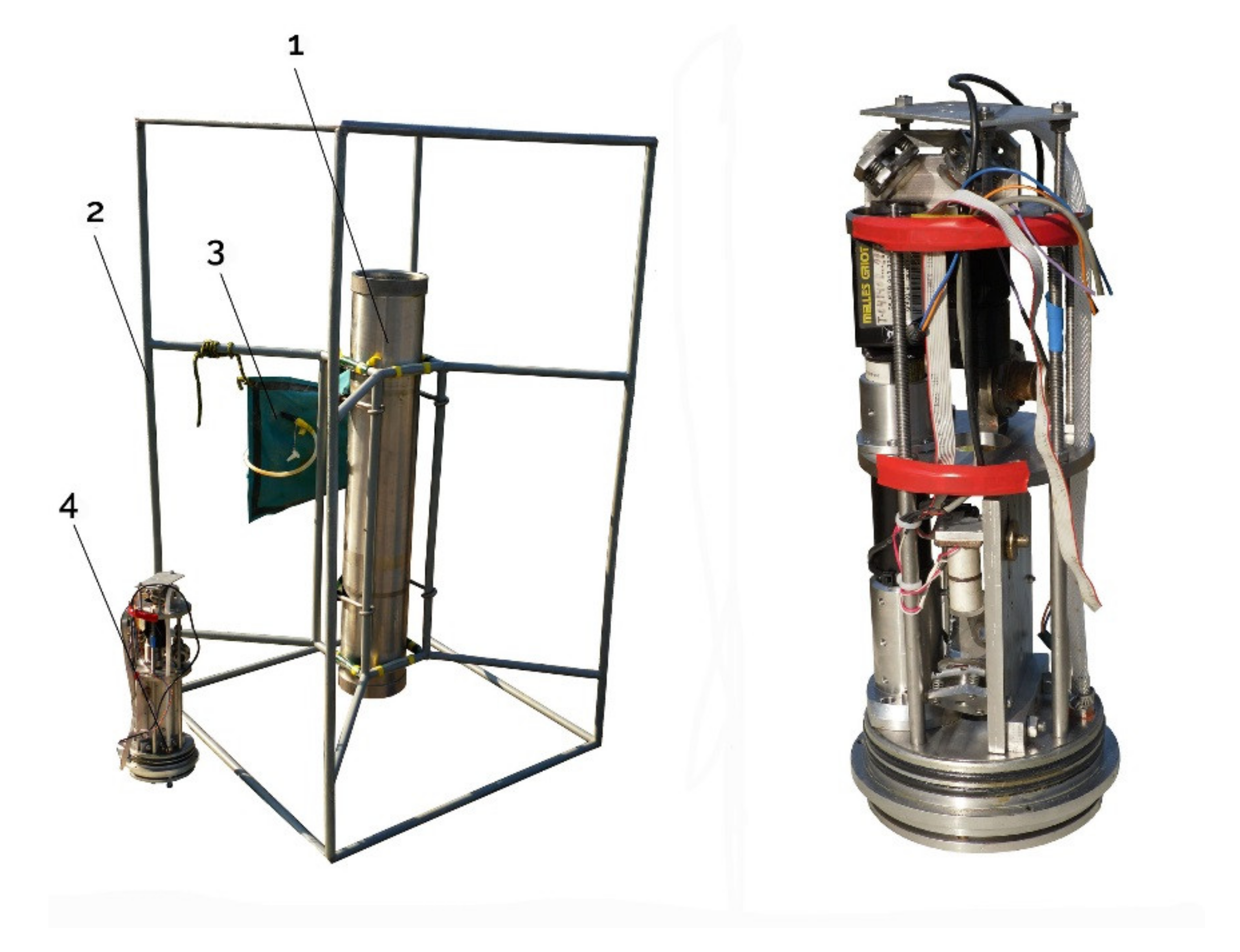Figure 2 shows the external view of the instrument, created based on the use of a modified Michelson interferometer of the homodyne type and a frequency-stabilized helium-neon laser, which ensures stability of the radiation frequency in the ninth decimal place. It is enclosed in a cylindrical stainless-steel housing, which is fastened in a protective grating designed to protect the instrument in severe operating conditions (rocky or slimy bottom). One side has a hole for cable entry. The other side is sealed with a lid. In addition to the protective grating, an elastic air-filled container is located outside the instrument. Its outlet is connected by a tube to a compensation chamber located in the removable cover. The housing contains a Michelson interferometer, the compensation chamber, an electromagnetic valve, and a digital recording system. The sensitive element of the supersensitive detector is the round stainless-steel membrane, which is fixed at the end face of the device. On the outside, the membrane interacts with water. A mirror is fixed on the thin pin inner side of the membrane, which is a part of the “cat’s eye” system, consisting of a biconvex lens with the appropriate focal length and this mirror. The mirror with the lens is included in the structure of the measuring arm of the interferometer. The mirror, rigidly fixed on a thin pin in the center of the membrane, shifts along the interferometer axis under the influence of the hydrosphere pressure variations. A change in the length of the measuring arm leads to the change in the intensity of the interference pattern, recorded by the digital registration system. The output signal of the supersensitive detector, after preprocessing by the digital registration system, is the hydrosphere pressure variations. It is possible to obtain the limiting technical characteristics of these systems by reducing photoelectronic equipment noise and the compensation of temperature noise, more accurately equalizing the length difference between the measuring and reference arms of the interferometer, which correspond to the following design parameters: an operating frequency range from 0 (conditionally) to 10,000 Hz, and a measuring accuracy of hydrosphere pressure variations 1.8 μPa.

Studying the dynamics and transformation of sea surface gravity waves at the shelf of decreasing depth, we will focus on the results of processing the experimental data, obtained when the laser meters of hydrosphere pressure variations were located at points 1, 2, and 3 (see Figure 3). Points 1 and 2 were in Vityaz Bay, the Sea of Japan, and point 3in the seaward part of the experimental site. At points 1 and 2 at the depths of 11.8 and 4.5 m, two laser meters of hydrosphere pressure variations were located at the same time, along the line perpendicular to the coastline in the instruments’ location area (perpendicular to the front of the surface gravity wave propagating from the deep-water part of Vityaz Bay towards the coastline). The distance between the systems was 96 m. At point 3, at the depth of 27 m, the laser meter of hydrosphere pressure variations was operating in the summer–autumn period of the year.

Additionally, we used the following equipment in the measuring complex: a TRIMBLE 5700 GPS, a meteorological station, low-frequency hydroacoustic emitters of an electromagnetic type, hydroacoustic receiving systems, hydrological profilers, and boats. The experimental data, obtained from all measuring systems, were transferred in real-time mode to the laboratory room, where, after filtration and decimation pre-processing, it was recorded on solid media with subsequent placement in the previously created experimental database.

3. Processing and Analysis of the Obtained Results

As appropriate, the results of the experimental studies, loaded into the experimental database, were processed further. Considering that the sampling frequency of the recorded data files was, in general, 1000 Hz, they were preliminarily filtered with a low-pass Hamming filter to the frequency of 1 Hz and further averaged to the sampling frequency of 2 Hz. The performed procedure allowed us to avoid the effect of power-consuming, high-frequency components overlapping the considered range of surface gravity sea waves (1–0.04 Hz). Depending on the planned processing results, various methods of experimental data processing were used: spectral methods (periodogram method, i.e., Fast Fourier Transform; the maximum likelihood method), averaging over different time windows with a suitable number of averagings, filtering with a high-frequency Hamming filter, statistical estimation methods, dynamic spectrogram.

Experimental studies of ocean wave processes in the range of surface gravity waves were carried out in the Sea of Japan. We know that periods of wind waves, and free wind waves–swell waves, depend on wind characteristics (speed, direction, duration), and also on the characteristics of the basin, over which a cyclone/typhoon is acting (geometrical dimensions of the sea, acceleration value, depth). For the Sea of Japan, the largest periods of wind waves are about 12–14 s, and background progressive surface gravity waves have periods of about 5–6 s. Therefore, these progressive waves, when interacting with the bottom, should generate primary microseisms of the corresponding periods (from 12–14 to 5–6 s). Standing surface waves should generate secondary microseisms with periods two times shorter than those of interacting progressive gravity waves. Further, we will not pay attention to these interactions and the formation of secondary microseisms in our work. Let us dwell on the dynamic changes of progressive gravity sea waves, as well as their transformation into primary microseisms. Figure 4 shows a dynamic spectrogram of a record of the laser meter of hydrosphere pressure variations in the range of sea progressive gravity waves. The data was obtained when registering swell waves, coming from the central areas of the Sea of Japan, where the speed of wind was high. The behavior of gravity sea waves shown in the figure is typical for all records of laser meters of hydrosphere pressure variations. As we can see from the figure, besides the linear component of the decrease in the period of wind waves (swell), there are also nonlinear components, associated with both a decrease and increase in the periods of wind waves.

The linear decrease in wind waves’ periods can be explained by dispersion, according to which free wind waves of large periods have high speeds. Therefore, the waves of large periods should be the first to reach the observer. For deep water, this ratio has the form:

$$c^2=\frac{g\lambda }{2\pi },$$

(1)

where $c$ is speed, $g$ is gravitational acceleration, $\lambda$ is a wavelength, $\lambda =g{T}^2/2\pi$, and $T$ is a wave period. When a wave moves in shallow water, the situation will not change much, since

$$c^2=gh,$$

(2)

where $h$ is sea depth in the wave propagation place. The following question is interesting: what mechanisms/processes cause the nonlinear change in the waves’ periods over time? We will disregard a possible slight increase in the periods during the initial phase, which is associated with a slight increase in the periods of swell after it leaves the wind zone due to attenuation of the high-frequency components and the energy transfer to the lower-frequency components. Let us consider the change in the periods of surface gravity waves when they propagate in the remaining deep-water part and at the shelf of decreasing depth. The change in the periods of surface gravity waves as they move through the rest of deep water can be partially associated with the Doppler Effect [17]. Analysis of the data of many months convinces us that the increase and decrease in the periods of wind waves, along with the mechanisms of developing waves and dispersion, are associated with the degree of change in the magnitude and direction of the speed of typhoons or other pressure depressions. That is, the change in the periods of wind waves is associated with the Doppler Effect. In accordance with the Doppler Effect, we write the expression:

$$f=f_0(1\pm u/c)$$

(3)

where: $f$ is frequency of the received signal, $f_0$ is frequency of the emitted signal, $u$ is the speed of source movement (typhoon, etc.), $c$ is wind waves’ speed, and “+” is used when approaching, “-” when moving away. Here, are some calculations. Let $c=20$ m/s and $u=36$ km/h, then $\Delta f=\pm 0.5f_0$. At 72 km/h, $\Delta f=\pm 1.0f_0$. Changes in wave periods, associated with the Doppler Effect, were studied in detail in [18], using data from the laser strainmeter, which recorded primary microseisms, caused by gravity sea waves generated by a distant typhoon moving in the Pacific Ocean.

These changes in the swell periods can be associated with a typhoon moving at high speeds. However, how can we associate the observed variations in the periods of surface gravity waves in the case of an almost stationary location of a powerful cyclone as the “generator” of wind waves? Especially when surface gravity waves move at the shelf of decreasing depth?

Let us consider the results of processing synchronous records of two laser meters of hydrosphere pressure variations, located at points 1 and 2 (see Figure 3). The distance between the systems is 96 m, and they are installed at depths of 11.8 (point 2 in Figure 3) and 4.5 m (point 1 in Figure 3). In this case, the average bottom slope is about 7.6%. We will pay attention to the dynamics of wind waves with periods from 5 to 8 s. The length of one processed dataset is 8192 s. Considering that a wind wave covers the distance between two systems in no more than 10 s, we can state that during the length of one dataset of 8192 s, the data from these two systems is synchronous. It follows from the analysis of all processed data that the periods and energy of surface gravity waves decrease as they move from the position of the laser meter of hydrosphere pressure variations, located at the depth of 11.8 m (point 2 in Figure 3), to the position of another laser meter of hydrosphere pressure variations, located at the depth of 4.5 m (point 1 in Figure 3). When moving in this area, the wind wave transfers part of its energy to the upper layer of the sea Earth’s crust. This process is observed not only at significant levels, but also at small amplitudes of wind waves, which, with some approximation, can be considered nonlinear. When wind waves propagate in the studied area, the average percentage of changes in the periods of wind waves in the range of 5–6 s is about 6%, and the average percentage of changes in the periods of wind waves in the range of 6–7 s is about 7%. It is clear that this change in the periods of wind waves is associated not only with the length of a wind wave but also with its amplitude. Figure 5 shows, as a typical example of the dynamics of wind waves during their movement at the shelf of decreasing depth, the spectra of synchronous fragments of the record of laser meters of hydrosphere pressure variations, installed at points 1 and 2 (Figure 3). We can see that the main maximum of wind waves with a period of 6.45 s transforms into the maximum with a period of 6.00 s.

Let us look at other synchronous experimental data, obtained from the above systems. Taking into account the fact that the speed of wind waves in shallow water approximately equals 6–10 m/s, the pairs of record fragments of the laser meters of hydrosphere pressure variations were taken with a short time shift (about 10 s). Additionally, 10 synchronous record fragments were processed. The results of processing are listed in

Table 1. Experimental data.

№№	Period, s	Sea Depth, m	Wave-Length, m	Speed, m/s	Relative Pressure at the Bottom	Relative Wave Amplitude
1	4.90	11.8	36.26	7.4	414	0.160
	4.47	4.5	25.03	5.6	874	0.150
2	5.65	11.8	45.80	8.1	276	0.072
	5.15	4.5	30.40	5.9	440	0.065
3	5.50	11.8	44.00	8.0	285	0.079
	5.36	4.5	31.60	5.9	550	0.078
4	5.82	11.8	48.30	8.3	388	0.094
	5.58	4.5	33.50	6.0	640	0.088
5	6.17	11.8	52.40	8.5	561	0.120
	4.79	4.5	27.80	5.8	663	0.100
6	5.07	11.8	38.5	7.6	815	0.320
	4.71	4.5	26.85	5.7	1928	0.310
7	4.87	11.8	36.04	7.4	498	0.198
	4.58	4.5	26.11	5.7	1111	0.183
8	6.90	11.8	62.1	9.0	1449	0.261
	6.50	4.5	40.3	6.2	1798	0.226
9	6.4	11.8	55.68	8.7	2010	0.407
	6.2	4.5	37.82	6.1	2436	0.315
10	6.4	11.8	55.68	8.7	1865	0.278
	6.2	4.5	37.82	6.1	1996	0.258

. The wavelength and wave speed for these periods of wind waves and depths are taken from [18]. According to the formula below, taken from [18], relative amplitudes of sea gravity waves on the water surface were calculated from relative pressure amplitudes, measured by the instruments installed on the bottom:

$$P=\frac{g\rho a}{ch(kh)}$$

(4)

where $g$ is gravitational acceleration, $\rho$ is water density, $a$ is a wave amplitude, $k=2\pi /\lambda$ is the wave number, and $h$ is sea depth.

As we can see from Table 1, there are no special dependences between changes in the periods of wind waves and changes in the amplitudes of wind waves, except one: almost always, the decrease in the period of wind waves is associated with the decrease in the amplitudes of wind waves. We can note that for periods shorter than 6.2 s, there is an almost (on average) linear relationship between the percentage change of the periods of wind waves and the percentage change of the amplitudes of wind waves. For periods longer than 6.2 s, there is a nonlinear relationship—in percentage terms, the change in the amplitudes of wind waves is significantly greater than the change in the periods of wind waves. Let us consider the reasons for these changes. Calculations are carried out in accordance with the theory described in [18]. Yet, only linear cases are considered there, which is not correct. However, unfortunately, no one can analytically solve nonlinear equations in which all the forces acting on the water are taken into account. Therefore, we will use what we have, and will try to describe a possible reason for the period change, and to quantify this change. In addition, we will verify the obtained estimates using other field data. The change in the periods of wind waves when they move at the sloping shelf can be associated with the average value of integral pressure along the entire path of wave propagation (96 m). It is clear that the more water particles, moving under the action of the wind wave near the bottom, press on the bottom, the greater part of the wave energy will go to the bottom. Therefore, the energy carried into the bottom will be proportional to the total pressure exerted on the bottom by the sea wind wave in the studied area. Let us calculate the total pressure for the pairs of waves listed in Table 1. For each element of the pair, this total pressure can be estimated by the formula:

$$P_{сум}={\displaystyle {\int }_{h_2}^{h_1}\frac{g\rho a}{ch(kh)}dh}$$

(5)

Expression (5) can be presented as follows:

$$P_{сум}=\frac{g\rho a\lambda }{\pi }\left(arctg\left(e^{\frac{2\pi h_1}{\lambda }}\right)-arctg\left(e^{\frac{2\pi h_2}{\lambda }}\right)\right)$$

(6)

At $a$ = 1 for a sea wind wave with a wavelength of 48 m, we have $P_{tot}$ = 44.34 kPa, and for a sea wind wave with a wavelength of 66 m, we have $P_{tot}$ = 54.17 kPa. Thus, with continuous impact on the sea bottom of a total pressure of 7.39 kPa, in the first case, the wave period changes (decreases) by 1%, and for the second case, with continuous impact on the sea bottom of a total pressure of 7.74 kPa, the wave period changes (decreases) by 1%. That is, taking into account possible approximation errors, we can assume that with continuous impact of the sea wind wave of any period on the bottom at a total pressure of 7.56 kPa, its period changes (decreases) by 1%.

Next, let us consider another case of the dynamics of the sea wind wave period when the laser meter of hydrosphere pressure variations was installed at the depth of 27 m. The change in the wave period from 10.4 to 6.9 s occurred within 32.5 h. In accordance with [18], from the dispersion relation for the group velocity of wind and swell waves, we have:

$$c_g=\frac{gT}{4\pi }$$

(7)

Then, the distance to the place of generation of these waves can be calculated by the formula:

$$L=\frac{T_1}{T_0-T_1}\times \frac{g{T}_0}{4\pi }\Delta t$$

(8)

The place of generation should be approximately at the distance of 1871 km, i.e., outside the Sea of Japan. For the second case, when the wave period changes from 9.4 to 6.9 s with a time interval between them of 16.4 h, according to the dispersion Equation (7), we find that the source of wind waves should be located at a distance of about 1200 km. That is, in the first and second cases, the sources of wind waves should be located outside the Sea of Japan/the East Sea, which is impossible, because this sea is practically closed to wind waves from the open part of the Pacific Ocean. Of course, only the linear change in the period of wind waves, associated only with the dispersion relation, is taken into account here. The Doppler Effect and decrease in the period of wind waves due to friction of a wave (water particles, with a loss of energy of the latter) when moving at the shelf of decreasing depth are not taken into account.

With regard to our Expression (6) and the obtained estimated parameters of the change in the periods of wind waves due to friction of the wave particles on the sea bottom, let us estimate the possible change in the periods in the cases described in the previous paragraph, when the waves propagate from the depths $h=\lambda /2$ to $h=27$ m. We will assume that a wind wave with a period of 10.4 s has a wavelength (deep sea) of 169 m, a wind wave with a period of 6.9 s has a wavelength (deep sea) of 74 m, and a wind wave with a period of 9.4 s has a wavelength (deep sea) 138 m. Then, the total pressure acting on the bottom, with a wave amplitude equal to 1, for the wave with a period of 10.4 s equals 184.6 kPa. On the condition that when the total pressure on the bottom is equal to 7.56 kPa, the wave period will decrease by 1%, we obtain that at 184.6 kPa, the wave period should decrease by 24%, i.e., the initial period of the wave that “enters” the shelf at the sea depth of 169 m will equal 13.7 s, not 10.4 s. For a wave with a period of 6.9 m, through the same calculations, we see that when the wave “enters” the shelf at the sea depth of 74 m, its period should be 7.1 s, not 6.9 s. In the same way, for a wave with a period of 9.4 s, we see that when a wind wave “enters” the shelf at the sea depth of 138 m, its period should be not 9.4 s, but 11.2 s. Further, in accordance with (8), we calculate the possible distance to the source of wind waves for new, calculated period values. For the dynamics of wind waves with periods from 13.7 to 7.1 s within 32.5 h, this source should be located at a distance of 1340 km from the registration site (previously, it was 1871 km). For the dynamics of wind waves with periods from 11.2 to 7.1 s within 16.4 h, this source should be located at a distance of 890 km from the registration site (previously, it was 1200 km).

Now, let us discuss peculiarities of using Formula (6) for calculations. In all cases, we assumed that the wavelength at the registration point would be equal to the wavelength in “deep” water. In fact, this is not quite correct. Thus, we should modify our calculations, considering that the wavelength for the registration point (sea depth 27 m) in Expression (6) will be shorter. Second: in our calculations, we took wave amplitude as equal to 1 everywhere. This is not quite correct. For waves with periods of 13.7 and 7.1 s, they will be different at the registration point, even if we assume that they have left the pressure depression zone with equal amplitudes. During propagation even in the “deep” sea, the amplitude of the wave with a period of 13.7 s will decrease less than the amplitude of the wave with period of 7.1 s due to dissipative effects. Unfortunately, we cannot calculate the wavelengths at the sea depth of 27 m using the available theoretical formulas, since they were all obtained with a rough linear approximation and upon the condition that the wave period never changes, which is completely wrong. The only hope is to carry out a large-scale complex experiment to register spatio-temporal dynamics of wind waves’ parameters from the places of their origin to the places of breaking. In addition, taking into account the fact that the dispersion Equation (7) was obtained under the conditions of linear approximation, without taking into account the summands of higher orders and, moreover, without taking into account the influence of many forces, except for gravitational, we can state that it is correct only with some rough approximation. We can obtain the value of this approximation only by analyzing such experimental data, which, unfortunately, nobody in the world has received yet. In view of the above, we cannot accurately estimate, using the above formulas, how the period of wind waves changes with time at the registration point. We will try to obtain these estimates, further analyzing the obtained experimental data.

Let us now consider some other effects of nonlinear behavior of surface gravity waves. Figure 6 shows a dynamic spectrogram of the laser meter of hydrosphere pressure variations record, which clearly shows low-frequency modulation of sea gravity progressive waves by a 12-hour tide. In some works, for example [2,4], the nonlinear transformation of the periods of surface gravity waves is associated with inter-harmonic transfer. That is, energy transfer is only possible from harmonic to harmonic, i.e., abruptly, not smoothly. Let us study this transformation, using experimental data. Let us take a dataset, a certain processing result of which is shown in Figure 6. Let us carry out spectral processing of successive fragments of the laser meter of hydrosphere pressure variations record. We take these fragments with a noticeable overlap, when the beginning of the next record fragment is shifted a little from the beginning of the previous fragment. In this case, the concentration of the maximum energy should change smoothly between frequencies from one fragment to another or jump from one harmonic to another. As follows from Figure 6, and from the results of additional processing, we do not observe an abrupt change in the period of wind waves. This change in the period of wind waves occurs smoothly.

In conclusion, let us consider some regularities in the transformation of the energy of sea surface gravity waves into the energy of microdeformations of the upper layer of the sea Earth’s crust, i.e., into primary microseisms. Studying these processes, we will use the experimental data of synchronous records of the laser meter of hydrosphere pressure variations, installed in point 3 in Figure 3 at the depth of 27 m and the 52.5-meter laser strainmeter, installed in point 4 in Figure 3. We will be interested in the issues associated with zones of transformation of wind waves (swell waves) into primary microseisms, and we will also try to find some regularities that confirm or refute the above results. Please note that we consider as primary those microseisms which resulted from transformation of surface wind progressive waves. For the Sea of Japan, the periods of these waves are in the range of 5 to 15 s (approximately). Of course, during the propagation of progressive swell waves with periods of about 14 s, under special conditions, standing waves with a period of 7 s can occur, which will excite secondary microseisms with the same period. However, it is not important. Important is that the primary microseisms are generated by progressive sea waves. In the course of the same processing of synchronous experimental data, we noted that for all fragments, the spectra of microseismic range in the records of the laser strainmeter are wider than the spectra of the same frequency range in the records of the laser meter of hydrosphere pressure variations. As an example, Figure 7 shows the spectra of the synchronous fragments of these devices’ records.

As we can see in Figure 5, the periods of waves and the periods of microseisms are, with some approximation, equal, and their maximum energy is concentrated in the range of 9–11 s. Let us consider the regularities of transformation of swell waves into primary microseisms with different periods. On the synchronous records of the instruments, within some time intervals, we identified oscillations with periods from 8 to 12 s, and within other time intervals, oscillations with periods from 5 to 7 s. Further, we will consider dynamic spectrograms and spectra of records of the laser strainmeter and the laser meter of hydrosphere pressure variations of different duration.

On dynamic spectrograms and spectra of records of the laser strainmeter and the laser meter of hydrosphere pressure variations, oscillations with periods from 9 to 12 s are identified (see Figure 8). On the dynamic spectrogram of the laser strainmeter (Figure 8a), the amplitude of oscillations in the range from 9 to 11.5 s is several times higher than the amplitude of background oscillations, which we can see in the spectrum below. Within the same time interval, oscillations with similar periods were identified in the records of the laser meter of hydrosphere pressure variations. On the dynamic spectrogram of the laser meter of hydrosphere pressure variations (Figure 8c), the amplitude of oscillations in the periods ranging from 9 to 12 s is several times higher than the amplitude of background oscillations. On the spectrum of the instrument record, shown below, in this range of periods, the amplitude of oscillations is also several times higher than the amplitude of the background oscillations. During further processing and analysis, we found a large number of fragments of the laser strainmeter and the laser meter of hydrosphere pressure variations records, where oscillation periods of microseisms coincide with periods of wind waves. This effect was observed on the instruments’ records over several days of the experiment.

In the second fragment of the laser strainmeter and the laser meter of hydrosphere pressure variations records, we identified microseisms and wind waves with periods of about 6 s. When analyzing dynamic spectrograms and spectra of the laser strainmeter and the laser meter of hydrosphere pressure variations records, we found microseisms with periods from 4.5 to 6 s, while periods of wind waves ranged from 5.5 to 7 s. The dynamic spectrogram (Figure 9a) shows microseisms with periods from 5 to 6 s. On the spectrum of the laser strainmeter, shown below, in this range of periods, the amplitude of oscillations is also several times higher than the amplitude of background oscillations. On the dynamic spectrogram (Figure 9b), wind waves with periods from 6 to 7 s are identified, which is also confirmed by the record spectrum of the laser meter of hydrosphere pressure variations, where amplitudes of these oscillations are several times higher than amplitudes of background oscillations. Examining many other fragments of the laser strainmeter and the laser meter of hydrosphere pressure variations records, we found that microseisms with periods of about 6 s gradually transformed into microseisms with periods of about 5 s. Accordingly, the period of wind waves gradually decreased from 7 to 6 s.

The study of microseisms, using the data of the laser strainmeter, and of wind waves, using the data of the laser meter of hydrosphere pressure variations, showed that when wind waves’ periods were about 9 s, microseisms with the same periods were identified, and when there were wind waves with periods of about 6 s, the period of recorded microseisms was lower. It is related to the location of the measuring instruments. Wind waves move towards the coast through the area of the laser meter of hydrosphere pressure variations installation. The length of the wind wave with a period of about 9 s is several times greater than the depth of the instrument installation, and the energy transfer from the wind wave to the bottom begins to occur at a depth equal to or less than a half-wavelength. The length of the wind wave with a period of about 6 s is comparable with the depth of the instrument installation, and energy transfer occurs at a shallower depth. When a wind wave propagates at the shelf, it loses part of its energy when interacting with the bottom, and its energy is redistributed to a higher frequency range. This fact is confirmed by registration of microseisms with periods less than the periods of wind waves by the laser strainmeter. Moreover, we can assert that the zone of the most effective transformation of the wind waves energy into the energy of primary microseisms with periods of about 5–6 s is located at depths less than 27 m. Additionally, for progressive wind waves with periods of 9–10 s, such a zone is located near the depth of 27 m.

4. Conclusions

Over the course of processing synchronous experimental data from two spatially distanced laser meters of hydrosphere pressure variations, installed on the shelf of decreasing depth along a line perpendicular to the wave front, we found that a wind wave, propagating at the shelf of steadily decreasing depth, when interacting with the bottom, loses part of its energy (transfers it to the bottom), which leads to the transformation of the wave spectrum, and the energy in the spectrum is redistributed to a higher frequency region. The magnitudes of these changes depend not only on the lengths of wind waves and the degree of depth decrease, but also on their amplitudes. We have obtained an analytical equation for approximate estimation of the energy of a gravity wave, transformed into the energy of the upper layer of the Earth’s crust. However, this equation does not take into account the dynamic change in the amplitude and length of a sea wave. Further theoretical studies, we hope, will allow us to formulate an analytical equation based on experimental data, which will take into account all the dynamic parameters of a sea gravity wave. We have established that the average percent of changes in the wave periods depends on the wavelength (the initial period of the incoming wave), when propagating through a specific area: the longer the period of a wave, the greater its change. This effect is associated with the amplitude of oscillations of water particles near the bottom, which is greater for waves with large periods. Because of this, total water pressure on the bottom is greater for waves with a longer period (wavelength).

To clarify our results on the percentage change in the periods of gravity sea waves as they move along the shelf of decreasing depth, and to assess the relationship of this percentage change in the periods of gravity sea waves to the energy carried away into the bottom, additional multiscale experimental studies are required. To perform this, on the shelf of monotonically decreasing depth, one-type instruments should be placed perpendicular to the front of a gravity sea wave at different depths, at 5–7 points (preferably, laser meters of hydrosphere pressure variations). In addition, receiving systems must operate on land to record primary microseisms (in our case, laser strainmeters). Based on the obtained experimental data, we would be able to estimate: (1) the periods and amplitudes of the gravity sea waves of a particular train at each point, and (2) the speed of a gravity sea wave from point to point. Equation (5) should be transformed, taking into account different amplitudes and periods at each point, speed and length of waves from point to point, using the full dispersion ratio $c^2=(g\lambda /2\pi )th(2\pi h/\lambda )$, to derive the analytical equation. The result should be an equation, similar to Equation (5), with a triple integral on the right-hand side. It is the solution of this equation that will allow us to estimate the dynamics of sea gravity waves as they move along the shelf of decreasing depth of various configurations. The results of this solution are also useful in the applied field to accurately forecast the parameters of sea waves in specific regions of different water areas.

Based on additional synchronous data from the coastal laser strainmeter, we have established that sea progressive gravity waves excite primary microseisms of the corresponding periods. We have experimentally ascertained that the zones of transformation of gravity waves into microseisms depend on the periods of surface gravity waves and are associated with their length.