Prescribed Performance Control of Marine Surface Vessel Trajectory Tracking in Finite-Time with Full-State Constraints and Input Saturation

Abstract

This manuscript mainly solves a fully actuated marine surface vessel prescribed performance trajectory tracking control problem with full-state constraints and input saturation. The entire control design process is based on a backstepping technique. The prescribed performance control is introduced to embody the analytical relationship between the transient performance and steady-state performance of the system and the parameters. Meanwhile, a new finite time performance function is introduced to ensure that the performance of the system tracking error is constrained within the preset constraints in finite time, and the full-state constraints problem of the system can be solved simultaneously in the entire control design, at the same time without introducing additional theory and parameters. To solve the non-smooth input saturation function matrix is not differentiable, the smooth function matrix is introduced to replace the non-smooth characteristics. Combining the Moore-Penrose generalized inverse matrix to design the virtual control law, the dynamic surface control is introduced to avoid the complicated virtual control derivation process, and finally the actual control law is designed using the properties of Nussbaum function. In addition, in view of the uncertainties in the system, a fractional disturbance observer is designed to estimate it. With the proposed control, the full-state will never be violated constraints, and the system tracking error satisfies transient and steady-state performance. Compared with other methods, the simulation results show the effectiveness and advantages of the proposed method.

1. Introduction

In recent years, the trajectory tracking control of surface vessels has interested a wide range of scholars, becoming a theoretical and practical research topic. The trajectory tracking control problem of marine surface vessels is a typical vessel motion control problem. Trajectory tracking involves designing a control law and guiding the system to track the required time reference trajectory. It is of great significance in many scenarios such as reconnaissance, surveillance, and waypoint navigation.

From the perspective of actual vessel navigation safety, vessel system variables need to operate under a specific constraint. Once these constraints are violated, it may lead to system dynamic performance degradation, instability and even dangerous accidents. In recent years, the barrier Lyapunov function method for dealing with system variable constraints has been gradually developed [1,2,3,4,5,6,7,8,9], among which typical reference [6] solves the trajectory tracking control problem of a class of fully actuated vessel system with output or full-state constraints, respectively. Furthermore, the barrier Lyapunov function method can ensure that the system full-state will not violate the constraints, but this method can only solve the convergence region of the tracking error in theory, and cannot effectively restrict the dynamic process of the tracking error over time, which makes it difficult to satisfy the requirements of the dynamic characteristics of the control system, i.e., it ignores the transient performance and steady-state error performance of the system.

To solve the dynamic performance constraint problem, the typical solution is the prescribed performance control method. In [10,11,12,13,14], the prescribed performance method is used to solve the control problem of a class of nonlinear systems with dynamic performance constraints. In reference [15], the prescribed performance method was applied to the design of altitude controller and speed controller for morphing aircraft. In reference [16], a new performance function is constructed to solve finite-time prescribed performance trajectory tracking problem of dynamic positioning ship. It should be noted that these methods are for control when time tends to infinity and cannot satisfy the control objective in finite-time. Reference [17] solves a class of nonlinear system control problems that require dynamic performance of the system. It constructs a new type of performance function to make the tracking error converge in finite-time and satisfy the transient and steady-state requirements. However, it does not solve the system state constraint requirements under the requirement of dynamics.

The above problems can be summarized as the soft constraint problem of the system. However, the actual system actuator will lead to input saturation constraints due to physical factors, which can be attributed to the hard constraints of the system. For related work dealing with input saturation constraint [18,19,20,21,22], they focused on dynamic positioning (DP) ship system positioning control and underactuated vessel system tracking control and uncertain nonlinear system design the anti-saturation controller to compensate for the effects of input saturation. Reference [23] uses the asymmetric saturation approach to solve a kind of fully actuated surface vessel trajectory tracking problem.

In addition, the unknown time-varying disturbances in the system, including the external and internal uncertainties of the system, are also a problem that cannot be ignored. Many references do not take the disturbances into consideration in the entire process of control design. To solve this problem [24] proposed a robust adaptive neural controller for the dynamic positioning system, where ship unknown model dynamics and time-varying disturbances are compensated for by adaptive radial basis function (RBF) neural networks. In the presence of ship unknown dynamic parameters, unavailable velocities, and unknown time-varying disturbances, while [25] developed an adaptive robust output feedback controller for the DP system by incorporating adaptive RBF neural networks and the high-gain observer into the vectorial backstepping method. Reference [26] applied dynamic sliding mode control method to improve underwater vehicles (UVs) systems robustness under the effects of the ocean current and model uncertainties, similarly [27], combined with multiple sliding surfaces to solve a nonlinear single input-single output (SISO) system with matched and unmatched uncertainties.

From the perspective of nonlinear system design, backstepping is currently an important method. Backstepping can be combined with many methods, such as barrier Lyapunov function, prescribed performance, neural network/fuzzy system, sliding mode control, etc. Combined with the Lyapunov method, the stability of the closed-loop system can be guaranteed. The control design method in this paper is mainly based on backstepping technique, combined with prescribed performance and disturbance observer to solve the problem of finite time constraint of marine surface vessel trajectory tracking. The specific contributions of this manuscript can be summarized as follows:

(1)

The finite-time full-state prescribed performance method is introduced into the trajectory tracking control of marine surface vessel with full-state constraints.

(2)

The generalized inverse of the matrix is used to design the virtual control law. The auxiliary signal is constructed by the augmented system, and a piecewise smooth matrix and Nussbaum function are combined to design the control law of the system under the input saturation constraint.

(3)

The fractional order theory is used to construct a fractional order adaptive disturbance observer to estimate the uncertainties in the system, which improves the robustness of the system.

(4)

Using Lyapunov analysis method, all the closed-loop system signals are ensured to be bounded.

The organization structure of this manuscript are as follows: Section 2 and Section 3 present the mathematical symbols, preliminaries and problem formulation used in this manuscript. Section 4 is the trajectory tracking control design for marine surface vessel. Section 5 simulation verifies the valid of the proposed method in this manuscript. Section 6 is a discussion. Section 7 presents the conclusions of the full manuscript.

2. Mathematical Symbols and Preliminaries

This section will give the mathematical symbols and related preliminaries that will be used throughout the manuscript.

2.1. Mathematical Symbols

To facilitate calculation and analysis, $|\cdot |$ is defined as the absolute value of a scalar or vector, the absolute value of a vector is defined as the absolute value of each element or each component in the vector, i.e., for a vector $\mathit{a}\in R^n$, $\left|\mathit{a}\right|={[|a_1|,\cdots ,|a_n|]}^T$. For any vectors $\mathit{a}\in R^n$ and $\mathit{b}\in R^n$, $\left|\mathit{a}\right|<\mathit{b}$ means $a_i<b_i$$(i=1,2,\cdots ,n)$. ${\lambda }_{\min }(\cdot )$ and ${\lambda }_{\max }(\cdot )$ represents the maximum and minimum values in the eigenvalue vector in a square matrix $(\cdot )$. In addition, $R^n$ denotes the n-dimensional Euclidean space.

2.2. Preliminaries

Lemma 1.

[28] Define $N({\chi }_i)$ as the Nussbaum function, $V(\cdot )$ and ${\chi }_i(\cdot )$ as smooth functions in $[0, t_f)$, and $V(t)\ge 0$, $\forall t\in [0, t_f)$, then $V$satisfies the relationship as follows:

$$\begin{array}{c}V\le V(0)e^{-ct}+\frac{m}{c}(1-e^{-ct})\\ +\frac{e^{-ct}}{{\gamma }_{\chi }}{\displaystyle {\int }_0^t{\displaystyle \sum _{i=1}^n({\epsilon }_{i}N({\chi }_i)-1)}}{\dot{\chi }}_i{e}^{c\tau }d\tau \end{array}$$

(1)

where $c>0$, ${\gamma }_{\chi }>0$, ${\epsilon }_i>0$ and $m$ is a normal value, then $V(\cdot )$, ${\chi }_i(\cdot )$, and ${\displaystyle {\int }_0^t{\mathsf{\Sigma }}_{i=1}^n({\epsilon }_{i}N({\chi }_i)-1){\dot{\chi }}_i{e}^{c\tau }d\tau }$ are bounded on set $[0, t_f)$. Throughout this manuscript, $N(\chi )=e^{{\chi }^2}\cos (\pi \chi /2)$ is considered.

Lemma 2.

[22]. For any $\delta \in {\Re }^{+}$ and $x\in \Re$, the following inequality holds

$$0\le \left|x\right|-x\tanh \left(\frac{x}{\delta }\right)\le \kappa \delta ,$$

(2)

where $\kappa =0.2785$ satisfies $\kappa =e^{-(\kappa +1)}$.

3. Problem Formulation

Figure 1 shows the marine surface vessel (MSV) in its coordinate system [19]. The coordinate system with O as the origin O-X₀Y₀Z₀ is the Earth-fixed frame, also known as the North-East coordinate system, in which the direction of OX₀ axis is north, OY₀ axis is east, and the direction of OZ₀ axis is to the Earth center. The coordinate system A-XYZ with A as the origin is the body-fixed frame, which is also known as the moving coordinate system with the MSV. The origin A can also be called the position of the center of gravity of the MSV. The AX axis to the forward direction of the MSV, and the AY axis to the MSV. The right side of the forward direction is perpendicular to the AX axis, and the AZ axis is perpendicular to the AX axis and the AY axis, respectively. Then the MSV three-degree-of-freedom model is established as follows.

$$\begin{array}{l}\dot{\eta }=J(\eta )\upsilon \\ M\dot{\upsilon }+C(\upsilon )\upsilon +D(\upsilon )\upsilon =\tau (\phi )+d(t)\\ y=\eta \end{array},$$

(3)

where $J(\eta )=J(\psi )$, $\eta ={[x,y,\psi ]}^T$ is the NE positions $(x,y)$ and heading $\psi \in [0, 2\pi ]$ of the vessel, respectively; $\upsilon ={[u,v,r]}^T$ is denoted the body-fixed frame velocities $(u,v)$ and the yaw rate $r$ of the vessel, respectively. $R(\psi )$ is a transformation matrix defined by:

$$R(\psi )=\left[\begin{array}{ccc}\cos \psi & -\sin \psi & 0\\ \sin \psi & \cos \psi & 0\\ 0& 0& 1\end{array}\right],$$

(4)

with the property $\Vert R(\psi )\Vert =1$ and ${\mathit{R}}^{-1}(\psi )={\mathit{R}}^T(\psi )$. $M$, $C(\upsilon )$ and $D(\upsilon )$ represent the non-singular positive and definite inertia matrix of symmetric, the Coriolis matrix, and the damping matrix, respectively. $d(t)\in R^3$ is the unknown time-varying disturbances from the environment, consisting of disturbance forces in surge, sway and moment in yaw. Considering the physical limitations of the propulsion system, the equivalent control force and torque of the ship provided by the propulsion system are limited. This problem is described as:

$${\tau }_i({\varphi }_i)=\{\begin{array}{l}{\tau }_i^{+},{\varphi }_i>{\tau }_i^{+}\\ {\varphi }_i ,{\tau }_i^{-}\le {\varphi }_i\le {\tau }_i^{+}\\ {\tau }_i^{-},{\varphi }_i<{\tau }_i^{-}\end{array}i=1,2,3,$$

(5)

where ${\tau }_i^{+}>0$ and ${\tau }_i^{-}>0$ are the upper and lower bounds of the saturation constraint of the propulsion system, respectively; ${\varphi }_i$ is the command control signal calculated by the vessel control law, including the surge control force ${\varphi }_1$, the sway control force ${\varphi }_2$, and the yaw control torque ${\varphi }_3$.

Figure 1. The marine surface vessel in coordinate system.

For input saturation constraint (5), we augmented the system (3). For the convenience of subsequent control design derivation, we defined $C=C(\upsilon )$, $D=D(\upsilon )$ and $J=J(\eta )$.

Let ${\mathit{x}}_1=\eta$ and ${\mathit{x}}_2=\upsilon$, then the vessel system model (3) can be written as:

$$\begin{array}{l}{\dot{x}}_1=J{x}_2\\ {\dot{x}}_2=M^{-1}[g(\phi )-C{x}_2-D{x}_2+b]\\ \dot{\phi }=-c\phi +\Phi \\ y=x_1\end{array},$$

(6)

Then, $g(\phi )$ can be expressed as $g(\phi )=\tau (\phi )-\mu (\phi )$. Where $\mu (\phi )$ is a bounded function, satisfying $\Vert \mu (\phi )\Vert \le \overline{\mu }$, and $b=\mu (\phi )+d(t)$, $c>0$, and $\Phi$ is a auxiliary signal that we will design next. In this manuscript, a smooth matrix $g(\phi )$ is introduced to approximate the non-smooth matrix. However, $\dot{\upsilon }$ is relatively difficult to relate to $g(\phi )$, which is difficult for the actual control input signal design and stability analysis. Therefore, in order to solve this problem, an augmented system is introduced, i.e., the third Equation in (6) is introduced.

To effectively apply backstepping technique, we define $g(\phi )={[g_1,g_2,g_3]}^T$ as:

$$g_i({\phi }_i)=\{\begin{array}{l}{\tau }_i^{+}\tanh \left(\frac{{\phi }_i}{{\tau }_i^{+}}\right),{\phi }_i\ge 0\\ {\tau }_i^{-}\tanh \left(\frac{{\phi }_i}{{\tau }_i^{-}}\right),{\phi }_i<0 \end{array}$$

(7)

The control objective of this manuscript is the marine surface vessel system (3) with input saturation constraints and unknown time-varying disturbances, the system output variable ${\mathit{x}}_1$ tracks the desired target ${\mathit{x}}_d={\mathit{\eta }}_d$, and the system variable satisfies the constraint conditions, i.e., ${\mathit{x}}_i={[x_{i1},x_{i2},x_{i3}]}^T$, satisfying $\left|x_{1j}\right|<K_{c1j}$, $\left|x_{2j}\right|<K_{c2j}$, $i=1,2;j=1,2,3$. The tracking error of the closed-loop system satisfies the transient and steady-state performance in finite-time.

Assumption 1.

The unknown time-varying disturbance$d(t)$ is bounded and there is a constant vector $\overline{d}={[{\overline{d}}_1,{\overline{d}}_2,{\overline{d}}_3]}^T$, satisfying $|d(t)|\le \overline{d}$.

Remark 1.

Since the marine environment is constantly changing and has finite energy, the interference acting on marine surface vessel can be regarded as an unknown time-varying but bounded signal. Therefore, assumption 1 is reasonable.

Assumption 2.

The target trajectory of the vessel is bounded, and there are bounded first-order, second-order and third-order derivatives ${\dot{\eta }}_d$, ${\mathit{\eta }}_d^{(2)}$, ${\mathit{\eta }}_d^{(3)}$, that is, there is a compact set${\mathsf{\Omega }}_{{\eta }_d}=\{{\mathit{\eta }}_d^{(n)T}:|{\mathsf{\Sigma }}_{n=0}^3\left|\right|{\mathit{\eta }}_d^{(n)}|{|}^2\le B_0\}\subset {\Re }^{12}$, such that ${[{\eta }_d^T,{\dot{\eta }}_d^T,{\eta }_d^{(2)T},{\eta }_d^{(3)T}]}^T\in {\mathsf{\Omega }}_{{\eta }_d}$, where$B_0>0\in \Re$.

4. Control Design

In this section, we design the trajectory tracking control law for the marine surface vessel based on the backstepping prescribed performance method to achieve the control objective. Before the control design, the finite-time performance function is introduced. The entire control design process consists of three steps. In step 1, select the appropriate Lyapunov function to design the virtual control law so that the transient and steady-state performance of the system pose tracking error can satisfy the prescribed requirements; In step 2, as in step 1, an appropriate Lyapunov function is selected to design a virtual control law to make the transient and steady-state performance of the system velocity tracking error can satisfy the prescribed requirements. Further, select an appropriate method so that the full-state of the system does not violate the constraints, and use an adaptive estimation method to estimate the bounds of the total disturbances of the system; the last step is to design auxiliary signals to further design the actual control law. Finally, the stability of the closed-loop system is analyzed. To clearly describe the entire control design process, an intuitive control design block diagram is given as shown in Figure 2.

Figure 2. The block diagram of adaptive dynamic surface constraint control for marine surface vessel.

Before the control design begins, we give the following performance functions definition.

Definition 1.

Smooth performance function$\rho (t)$, for any $t\ge T_f$, simultaneously satisfies three properties: (1) $\rho (t)>0$; (2) $\dot{\rho }(t)\le 0$; (3) ${\lim }_{t\to T_f}\rho (t)={\rho }_{T_f}>0$and$\rho (t)={\rho }_{T_f}$ for any $t\ge T_f$, ${\rho }_{T_f}$and$T_f$are arbitrarily small constants and set time, respectively.

According to definition 1, the finite-time performance function is expressed as follows.

$$\rho (t)=\{\begin{array}{ll}({\rho }_0-\frac{t}{T_f})e^{(1-\frac{T_f}{T_f-t})}+{\rho }_{T_f},& t\in [0,T_f)\\ {\rho }_{T_f},& t\in [T_f,+\infty )\end{array},$$

(8)

where ${\rho }_0\ge 1$ and ${\rho }_{T_f}>0$ are design parameters. It is easy to see that the $\rho (t)$ finite-time performance function satisfies all the properties mentioned in Definition 1. It is easy to see that (8) satisfies all the properties mentioned in definition 1 and that the initial condition of $\rho (t)$ is $\rho (0)={\rho }_0+{\rho }_{T_f}$. The smoothness proof is given below.

Proof of Smoothness 1.

When $t\ge T_f$, $i\ge 1$, $\frac{{\partial }^i[\rho (t)]}{\partial t^i}=0$ means $\frac{{\partial }^i[\rho (t)]}{\partial t^i}$ is continuous and $\underset{t\to T_f^{+}}{\lim }\frac{{\partial }^i[\rho (t)]}{\partial t^i}=0$. Let ${\rho }_0-\frac{t}{T_f}=v(t)$, $1-\frac{T_f}{T_f-t}=\frac{t}{t-T_f}=w(t)$, $\rho (t)$ can be rewritten as $\rho (t)=v(t)e^{w(t)}+{\rho }_{T_f}$. □

(a). Taking the derivative $\rho (t)$ with respect to time $t$, and using $v(t)$ and $w(t)$ and L ‘Hopital’s rule, we get:

$$\underset{t\to T_f^{+}}{\lim }\frac{\partial \rho (t)}{\partial t}=\underset{t\to T_f^{-}}{\lim }\frac{\partial \rho (t)}{\partial t}=0$$

(9)

This shows that $\frac{\partial \rho (t)}{\partial t}$ is continuous and $\rho (t)$ is differentiable.

(b). Take the second derivative $\rho (t)$ with respect to time $t$, and we get

$$\frac{{\partial }^2\rho (t)}{\partial t^2}=\frac{d^{2}v(t)}{d{t}^2}{e}^{w(t)}+2\frac{dv(t)}{dt}\frac{dw(t)}{dt}{e}^{w(t)}+v(t)\frac{d^{2}v(t)}{d{t}^2}{e}^{w(t)}+v(t){\left(\frac{dw(t)}{dt}\right)}^2{e}^{w(t)},$$

(10)

where $\underset{t\to T_f^{-}}{\lim }\frac{d^{2}v(t)}{d{t}^2}{e}^{w(t)}=0$, $\underset{t\to T_f^{-}}{\lim }\frac{dv(t)}{dt}\frac{dw(t)}{dt}{e}^{w(t)}=0$, $\underset{t\to T_f^{-}}{\lim }\frac{d^{2}w(t)}{d{t}^2}{e}^{w(t)}=\underset{t\to T_f^{-}}{\lim }\frac{\frac{{\varsigma }_2}{{(t-T_f)}^3}}{e^{-\frac{t}{t-T_f}}}=0$, $\underset{t\to T_f^{-}}{\lim }{(\frac{dw(t)}{dt})}^2{e}^{w(t)}=\underset{t\to T_f^{-}}{\lim }\frac{\frac{1}{{(t-T_f)}^4}}{e^{-\frac{t}{t-T_f}}}=0$.

Take the limit of Equation (10) at $t\to T_f^{-}$, and we get $\underset{t\to T_f^{-}}{\lim }\frac{{\partial }^2\rho (t)}{\partial t^2}=0$. Therefore, $\frac{{\partial }^2\rho (t)}{\partial t^2}=0$ is continuous and $\rho (t)$ is secondarily differentiable.

(c). $\frac{{\partial }^i\rho (t)}{\partial t^i}(i=3, \cdot \cdot \cdot , n-1)$ can be expressed as a polynomial of $\frac{1}{{(t-T_f)}^r}{e}^{w(t)}$ and $\frac{d^{\upsilon }v(t)}{d{t}^{\upsilon }}$, so $r\ge 0$, $\upsilon \ge 0$, and through a and b, and then we get:

$$\underset{t\to T_f^{-}}{\lim }{e}^{w(t)}\frac{1}{{(t-T_f)}^r}=\underset{t\to T_f^{-}}{\lim }\frac{\frac{1}{{(t-T_f)}^r}}{e^{-\frac{t}{t-T_f}}}=\frac{{\displaystyle {\prod }_{j=0}^r(r-j)}}{T_f^r}\underset{t\to T_f^{-}}{\lim }{e}^{w(t)}=0,$$

(11)

together with $\underset{t\to T_f^{-}}{\lim }{e}^{w(t)}=\underset{t\to T_f^{-}}{\lim }\frac{d^{i}v(t)}{d{t}^i}=0$, $i=3,\cdot \cdot \cdot ,n-1$, we can get $\underset{t\to T_f^{-}}{\lim }\frac{{\partial }^i\rho (t)}{\partial t^i}=0$. Similarly, since $\underset{t\to T_f^{+}}{\lim }\frac{{\partial }_i^i\rho (t)}{\partial t^i}=\underset{t\to T_f^{+}}{\lim }\frac{{\partial }_i^i\rho (t)}{\partial t^i}=0$ leads to $\frac{{\partial }^i\rho (t)}{\partial t^i}$ being continuous, $\rho (t)$ is $i$ times differentiable. In this way, by settling $i$ to $n$, it is easy to know that $\underset{t\to T_f^{-}}{\lim }\frac{{\partial }^n\rho (t)}{\partial t^n}=0$ holds. Therefore, the finite-time performance function $\rho (t)$ is nth differentiable and smooth, and the proof is complete.

It should be emphasized that the key difference between (8) and ${\rho }_1(t)=({\rho }_0-{\rho }_{\infty })e^{-\varpi t}+{\rho }_{\infty }$ or ${\rho }_2(t)=\coth (\epsilon t+\gamma )-1+{\rho }_{\infty }$ is the property of finite time convergence, but the traditional performance functions ${\rho }_1(t)$ and ${\rho }_2(t)$ do not have this property in [14,29], where ${\rho }_0$, ${\rho }_{\infty }$, $\epsilon$ and $\gamma$ are normal numbers.

4.1. Controller Design

The nonlinear function is introduced as follows

$${\epsilon }_{ij}(t)=\log \left(\frac{{\delta }_{ij}+{\xi }_{ij}}{{\delta }_{ij}-{\xi }_{ij}}\right),$$

(12)

where $0<{\delta }_{ij}\le 1$, $t\in [0,\infty )$, $i=1,2;j=1,2,3$. ${\xi }_{ij}$ is defined as ${\xi }_{ij}=\frac{z_{ij}}{{\rho }_{ij}}$. The form of ${\rho }_{ij}$ is shown in (8). Next, an adaptive dynamic surface controller is designed for the augmented system (6) with backstepping:

Step 1: Considering the first subsystem system in the augmented system (6) and defining the pose tracking error as follows.

$$z_{1j}(t)=x_{1j}(t)-x_{dj}(t),j=1,2,3,$$

(13)

where $x_{1j}$ is the j-th component of $x_1$, and $x_{dj}$ is the j-th component of $x_d$. The initial condition of ${\rho }_{1j}(t)$ satisfies ${\rho }_{1j}(0)\ge |z_{1j}(0)|=|x_{1j}(0)-x_{dj}(0)|$.

To satisfy the output tracking error dynamics in the control objective, that is, $-{\delta }_{ij}{\rho }_{ij}(t)<z_{ij}(t)<{\delta }_{ij}{\rho }_{ij}(t),i=1;j=1,2,3$, we select the candidate Lyapunov function for the first subsystem as follows:

$$V_0=\frac{1}{2}{\epsilon }_1^T{\epsilon }_1,$$

(14)

where ${\epsilon }_1={[{\epsilon }_{11},{\epsilon }_{12},{\epsilon }_{13}]}^T$. From Equation (12), we know that that for $\left|{\xi }_{1j}\right|<{\delta }_{1j}$, $V_0$ is strictly positive definite and differentiable, then $V_0$ is a valid candidate Lyapunov function.

Following the trajectories of the solutions of (14), taking the derivative with respect to time $t$, we get:

$$V_0={\epsilon }_1^T{\dot{\epsilon }}_1$$

(15)

According to Equation (15), the derivative of ${\epsilon }_1$ is required. Therefore, when $i=1$, the derivative of Equation (12) is obtained:

$${\dot{\epsilon }}_{1j}=\frac{2{\delta }_{1j}{\dot{\xi }}_{1j}}{{\delta }_{1j}^2-{\xi }_{1j}^2}$$

(16)

The derivative of ${\xi }_{1j}$ with respect to time $t$ according to (16) is then obtained:

$${\dot{\xi }}_{1j}=\frac{1}{{\rho }_{1j}}({\dot{z}}_{1j}-{\dot{\rho }}_{1j}{\xi }_{1j})$$

(17)

According to (15)–(17), we get:

$${\dot{V}}_0={\epsilon }_1^T{\Lambda }_1({\dot{x}}_1-{\dot{x}}_d-{\dot{\rho }}_1{\xi }_1),$$

(18)

where ${\Lambda }_1=diag\left(\frac{{\delta }_{11}}{({\delta }_{11}^2-{\xi }_{11}^2){\rho }_{11}},\frac{{\delta }_{12}}{({\delta }_{12}^2-{\xi }_{12}^2){\rho }_{12}},\frac{{\delta }_{13}}{({\delta }_{13}^2-{\xi }_{13}^2){\rho }_{13}}\right)$ and ${\dot{\rho }}_1{\xi }_1={[{\dot{\rho }}_{11}{\xi }_{11},{\dot{\rho }}_{12}{\xi }_{12},{\dot{\rho }}_{13}{\xi }_{13}]}^T$.

For the second subsystem in the augmented system (6), define the velocity tracking error as follows:

$$z_{2j}(t)=x_{2j}(t)-{\alpha }_{1j}(t),j=1,2,3,$$

(19)

where ${\alpha }_{1j}$ is the output of the first-order filter. To apply the dynamic surface technique, let the virtual control law $I_{{\alpha }_1}={[I_{\alpha 11},I_{\alpha 12},I_{\alpha 13}]}^T\in {\Re }^3$ to be designed, which is also the input of the first-order filter, through the following first-order filter.

$${\pi }_1{\dot{\alpha }}_1+{\alpha }_1=I_{{\alpha }_1},{\alpha }_1(0)=I_{{\alpha }_1}(0),$$

(20)

where ${\alpha }_1={[{\alpha }_{11},{\alpha }_{12},{\alpha }_{13}]}^T\in {\Re }^3$ is the output state vector of the first-order filter, and ${\pi }_1>0$ is the design constant. Meanwhile, we define the boundary layer as follows.

$$Y_1={\alpha }_1-I_{\alpha 1}$$

(21)

To design the virtual control law $I_{{\alpha }_1}$, we consider the following candidate Lyapunov function:

$$V_1=V_0+\frac{1}{2}{Y}_1^T{Y}_1$$

(22)

Following the trajectories of the solutions of (22), take the derivative of $V_1$ with respect to time $t$, and substitute $Y_1$ and $z_2$ to obtain:

$$\begin{array}{cc}\hfill {\dot{V}}_1& ={\epsilon }_1^T{\Lambda }_1[\mathit{J}(z_2+Y_1+I_{\alpha 1})-{\dot{x}}_d-{\dot{\rho }}_1{\xi }_1]+Y_1^T{\dot{Y}}_1\hfill \\ & \le {\epsilon }_1^T{\Lambda }_1\mathit{J}{z}_2+\frac{1}{2}{\epsilon }_1^T{\Lambda }_1{\Lambda }_1^T{\epsilon }_1+\frac{1}{2}{Y}_1^T{Y}_1+{\epsilon }_1^T{\Lambda }_1\mathit{J}{I}_{\alpha 1}\hfill \\ & -{\epsilon }_1^T{\Lambda }_1{\dot{x}}_d-{\epsilon }_1^T{\Lambda }_1{\dot{\rho }}_1{\xi }_1+Y_1^T{\dot{Y}}_1\hfill \end{array}$$

(23)

According to Definition 1, ${\rho }_{1j}$ is bounded. According to the extreme value theory of continuous function, it is easy to know that for $\left|{\xi }_{1j}\right|<{\delta }_{1j}$, there is a positive definite diagonal matrix ${\Lambda }_1$ and every element in ${\Lambda }_1$ is greater than zero and bounded. Therefore, there is an invertible matrix ${\Lambda }_1^{-1}$, so the virtual control law $I_{{\alpha }_1}$ is designed as follows:

$$I_{\alpha 1}=J^{-1}\left(-K_1{\Lambda }_1^{-1}{\epsilon }_1-\frac{1}{2}{\Lambda }_1^T{\epsilon }_1+{\dot{x}}_d+{\dot{\rho }}_1{\xi }_1\right),$$

(24)

where $K_1=diag(k_{11},k_{12},k_{13})$ is a positive definite design matrix, and according to Young’s inequality, we have the following inequality holds.

$$\frac{1}{2}{Y}_1^T{Y}_1+Y_1^T{\dot{Y}}_1=\left(\frac{1}{2}-\frac{1}{{\varsigma }_1}\right)Y_1^T{Y}_1-Y_1^T{\dot{I}}_{\alpha 1}\le \left(\frac{1}{2}-\frac{1}{{\varsigma }_1}+\frac{{\varpi }_1^2}{{\iota }_1^2}\right)Y_1^T{Y}_1+\frac{{\iota }_1^2}{4},$$

(25)

where ${\varpi }_1>0$ is a constant such that ${\varpi }_1\ge \Vert {\dot{I}}_{\alpha 1}\Vert$, and ${\iota }_1$ is a constant to be designed.

Substituting the virtual control law $I_{{\alpha }_1}$ and (25) into ${\dot{V}}_1$ to obtain:

$${\dot{V}}_1\le -{\epsilon }_1^T{K}_1{\epsilon }_1+{\epsilon }_1^T{\Lambda }_1\mathit{J}{z}_2-\left(\frac{1}{{\varsigma }_1}-\frac{1}{2}-\frac{{\varpi }_1^2}{{\iota }_1^2}\right)Y_1^T{Y}_1+\frac{{\iota }_1^2}{4},$$

(26)

where, item ${\epsilon }_1^T{\Lambda }_1\mathit{J}{z}_2$ in (26) will be eliminated in Step 2.

Step 2: Select the performance function ${\rho }_{2j}(t)$ for the second subsystem in the augmented system (6) and the initial condition satisfies ${\rho }_{2j}(0)\ge |z_{2j}(0)|=|x_{2j}(0)-{\alpha }_{1j}(0)|$. According to the error system $z_2=x_2-{\alpha }_1$, we get:

$${\dot{z}}_2=M^{-1}[\mathit{g}(\mathit{\phi })-\mathit{C}{x}_2-\mathit{D}{x}_2+\mathit{b}]-{\dot{\alpha }}_1$$

(27)

For the third subsystem in the augmented system (6), the error vector $z_3$ is defined as follows:

$$z_3=\mathit{g}(\mathit{\phi })-{\alpha }_2,$$

(28)

where ${\alpha }_2={[{\alpha }_{21},{\alpha }_{22},{\alpha }_{23}]}^T\in {\Re }^3$ is the output state vector of the first-order filter. Similarly, in order to apply dynamic surface technique, we let the virtual control law to be designed also be the input $I_{{\alpha }_2}={[I_{\alpha 21},I_{\alpha 22},I_{\alpha 23}]}^T\in {\Re }^3$ of the first-order filter through the following first-order filter.

$${\pi }_2{\dot{\alpha }}_2+{\alpha }_2=I_{{\alpha }_2},{\alpha }_2(0)=I_{{\alpha }_2}(0),$$

(29)

where ${\pi }_2>0$ is the design constant.

Remark 2.

The state differential term${\alpha }_i$ of the filter can be obtained directly from$(I_{\alpha i}-{\alpha }_i)/{\pi }_i$to replace the first derivative term of$I_{{\alpha }_i}$$(i=1,2)$. That is to say, in the process of traditional backstepping design, this fraction replaces${\dot{\alpha }}_i$. The purpose of doing this is to replace differential operation by simple algebraic operation, which simplifies the structure of the control law and makes it easier for engineering implementation.

We define the boundary layer as follows:

$$Y_2={\alpha }_2-I_{\alpha 2}$$

(30)

From assumption 1, it can be known that the time-varying disturbance $\mathit{b}\in {\Re }^3$ satisfies $|\mathit{b}|\le \mathit{\sigma }$. Since $M$ is a positive definite symmetric matrix, we set $M^{-1}\left|\mathit{b}\right|\le M^{-1}\mathit{\sigma }=\mathit{\theta }$, and define $\widehat{\theta }$ and $\tilde{\theta }=\widehat{\theta }-\mathit{\theta }$ as the estimation vector and estimation error vector of $\theta$.

To design the virtual control law $I_{{\alpha }_2}$ and the adaptive law $\dot{\widehat{\theta }}$, we consider the candidate Lyapunov functions as follows:

$$V_2=\frac{1}{2}{\epsilon }_2^T{\epsilon }_2+\frac{1}{2}{Y}_2^T{Y}_2+\frac{1}{2{\gamma }_{\theta }}{\tilde{\theta }}^T\tilde{\theta },$$

(31)

where ${\epsilon }_2={[{\epsilon }_{21},{\epsilon }_{22},{\epsilon }_{23}]}^T$, ${\gamma }_{\theta }>0$ is the adjustable parameter. It can be seen from Equation (12) that $V_2$ is strictly positive definite and differentiable for $\left|{\xi }_{2j}\right|<{\delta }_{2j}$, then $V_2$ is also a valid candidate Lyapunov function. Following the trajectories of the solutions of (31), take the derivative of $V_2$ with respect to time $t$, and we can obtain:

$${\dot{V}}_2={\epsilon }_2^T{\dot{\epsilon }}_2+Y_2^T{\dot{Y}}_2+\frac{1}{{\gamma }_{\theta }}{\tilde{\theta }}^T\dot{\widehat{\theta }}$$

(32)

We first deal with the derivative of ${\dot{\epsilon }}_2$. When $i=2$, taking the derivative of Equation (12), we get:

$${\dot{\epsilon }}_{2j}=\frac{2{\delta }_{2j}{\dot{\xi }}_{2j}}{{\delta }_{2j}^2-{\xi }_{2j}^2}$$

(33)

Then take the derivative of ${\xi }_{2j}$ with respect to time $t$ according to (33), and get:

$${\dot{\xi }}_{2j}=\frac{1}{{\rho }_{2j}}({\dot{z}}_{2j}-{\dot{\rho }}_{2j}{\xi }_{2j})$$

(34)

According to (28), (30), and (32)–(34), we can get:

$$\begin{array}{ll}{\dot{V}}_2& ={\epsilon }_2^T{\Lambda }_2[M^{-1}(\mathit{g}(\mathit{\phi })-\mathit{C}{x}_2-\mathit{D}{x}_2+\mathit{b})-{\dot{\alpha }}_1-{\dot{\rho }}_2{\xi }_2]+Y_2^T{\dot{Y}}_2+\frac{1}{{\gamma }_{\theta }}{\tilde{\theta }}^T\dot{\widehat{\theta }},\\ & ={\epsilon }_2^T{\Lambda }_2[M^{-1}(z_3+Y_2+I_{\alpha 2}-\mathit{C}{x}_2-\mathit{D}{x}_2+\mathit{b})-{\dot{\alpha }}_1-{\dot{\rho }}_2{\xi }_2]+Y_2^T{\dot{Y}}_2+\frac{1}{{\gamma }_{\theta }}{\tilde{\theta }}^T\dot{\widehat{\theta }}\\ & \le {\epsilon }_2^T{\Lambda }_2{M}^{-1}{I}_{\alpha 2}-{\epsilon }_2^T{\Lambda }_2{M}^{-1}[C{x}_2+D{x}_2-b+M{\dot{\alpha }}_1+M{\dot{\rho }}_2{\xi }_2]\\ & +{\epsilon }_2^T{\Lambda }_2{M}^{-1}{z}_3+\frac{1}{2}{\epsilon }_2^T{\Lambda }_2{M}^{-1}{(M^{-1})}^T{\Lambda }_2^T{\epsilon }_2+\frac{1}{2}{Y}_2^T{Y}_2+Y_2^T{\dot{Y}}_2+\frac{1}{{\gamma }_{\theta }}{\tilde{\theta }}^T\dot{\widehat{\theta }}\end{array},$$

(35)

where:

${\Lambda }_2=diag\left(\frac{{\delta }_{21}}{({\delta }_{21}^2-{\xi }_{21}^2){\rho }_{21}(t)},\frac{{\delta }_{22}}{({\delta }_{22}^2-{\xi }_{22}^2){\rho }_{22}(t)},\frac{{\delta }_{23}}{({\delta }_{23}^2-{\xi }_{23}^2){\rho }_{23}(t)}\right)$, ${\dot{\rho }}_2{\xi }_2={[{\dot{\rho }}_{21}{\xi }_{21},{\dot{\rho }}_{22}{\xi }_{22},{\dot{\rho }}_{23}{\xi }_{23}]}^T$.

Similarly, according to definition 1, ${\rho }_{2j}$ is bounded. According to the extreme value theory of continuous functions, it is easy to know that for $\left|{\xi }_{2j}\right|<{\delta }_{2j}$, ${\Lambda }_2$ is a positive definite diagonal matrix and each element in ${\Lambda }_2$ is greater than zero and bounded. Therefore, there is an invertible matrix ${\Lambda }_2^{-1}$, and using Lemma 2, we have the following inequality holds:

$${\epsilon }_2^T{\Lambda }_2{M}^{-1}\mathit{b}\le {\displaystyle \sum _{j=1}^3\left|{\epsilon }_{2j}\right|{\Lambda }_{2j}{\theta }_j}\le {\displaystyle \sum _{j=1}^3\left[{\epsilon }_{2j}\tan h\left(\frac{{\epsilon }_{2j}}{ƛ}\right){\Lambda }_{2j}{\theta }_j+\kappa ƛ{\Lambda }_{2j}{\theta }_j\right]}={\epsilon }_2^T\mathrm{Tanh}\left(\frac{{\epsilon }_2}{ƛ}\right){\Lambda }_2\mathit{\theta }+d^{\prime }$$

(36)

In inequality (36), $\mathrm{Tanh}(\frac{{\epsilon }_2}{ƛ})=diag(\tan h(\frac{{\epsilon }_{21}}{ƛ}),\tan h(\frac{{\epsilon }_{22}}{ƛ}),\tan h(\frac{{\epsilon }_{23}}{ƛ}))$ and $d^{\prime }=\kappa ƛ{\mathsf{\Sigma }}_{j=1}^3{\Lambda }_{2j}{\theta }_j$. Then inequality (35) can be written as:

$$\begin{array}{cc}\hfill {\dot{V}}_2& \le {\epsilon }_2^T{\Lambda }_2{M}^{-1}{I}_{\alpha 2}-{\epsilon }_2^T{\Lambda }_2{M}^{-1}\left[C{x}_2+D{x}_2+M{\dot{\alpha }}_1+M{\dot{\rho }}_2{\xi }_2\right]\hfill \\ & +{\epsilon }_2^T{\Lambda }_2{M}^{-1}{z}_3+\frac{1}{2}{\epsilon }_2^T{\Lambda }_2{M}^{-1}{(M^{-1})}^T{\Lambda }_2^T{\epsilon }_2+\frac{1}{2}{Y}_2^T{Y}_2+Y_2^T{\dot{Y}}_2\hfill \\ & +{\epsilon }_2^T\mathrm{Tanh}\left(\frac{{\epsilon }_2}{ƛ}\right){\Lambda }_2\theta +d^{\prime }+\frac{1}{{\gamma }_{\theta }}{\tilde{\theta }}^T\dot{\widehat{\theta }}\hfill \end{array}$$

(37)

According to the Moore-Penrose generalized inverse ${({\epsilon }_2^T)}^{+}$ of matrix ${\epsilon }_2^T$, yields:

$${\epsilon }_2^T{({\epsilon }_2^T)}^{+}=\{\begin{array}{l}0, \mathrm{if} {\epsilon }_2=0_{3\times 1}\\ 1, \mathrm{otherwise}\end{array}$$

(38)

When ${\epsilon }_2^T{({\epsilon }_2^T)}^{+}=0$, we know that ${\epsilon }_2=0_{3\times 1}$, which means that when ${\epsilon }_{2i}=0$, according to Equation (12), we know that ${\xi }_{2j}=0$, that is, $z_{2j}=0$, $j=1,2,3$. Then, when $z_{2j}=0$ and ${\dot{V}}_2=-{\mathsf{\Sigma }}_{j=1}^3{k}_{1j}{\epsilon }_{1j}^2\le 0$, the pose tracking error will converge to the prescribed region in finite time $T_f$. When ${\epsilon }_2^T{({\epsilon }_2^T)}^{+}=1$, it can be known that ${\epsilon }_2\ne 0_{3\times 1}$. We design the virtual control law and adaptive law of the second subsystem as follows:

$$\begin{array}{c}{I}_{\alpha 2}=-M{\Lambda }_2^{-1}{({\epsilon }_2^T)}^{+}{\epsilon }_1^T{\Lambda }_{1}J{z}_2-M{K}_2{\Lambda }_2^{-1}{\epsilon }_2-\frac{1}{2}{(M^{-1})}^T{\Lambda }_2^T{\epsilon }_2\\ +C{x}_2+D{x}_2+M{\dot{\alpha }}_1+M{\dot{\rho }}_2{\xi }_2-MTanh\left(\frac{{\epsilon }_2}{ƛ}\right)\widehat{\theta }\end{array},$$

(39)

$$\dot{\widehat{\theta }}={\gamma }_{\theta }\left[\mathrm{Tanh}\left(\frac{{\epsilon }_2}{ƛ}\right){\Lambda }_2{\epsilon }_2-{\lambda }_{\theta }\widehat{\theta }\right],$$

(40)

where $K_2=diag(k_{21},k_{22},k_{23})$ is a positive definite design matrix, and ${\lambda }_{\theta }>0$ is a constant design parameter.

In summary, we define the following function:

$$H(z_2)=\{\begin{array}{l}0, z_2=0_{3\times 1}\\ 1, \mathrm{otherwise}\end{array}$$

(41)

Finally, the virtual control law $I_{{\alpha }_2}$ and adaptive law $\dot{\widehat{\theta }}$ of the second subsystem are expressed as follows:

$$I_{\alpha 2}=H(z_2)\left\{\begin{array}{l}-M{\Lambda }_2^{-1}{({\epsilon }_2^T)}^{+}{\epsilon }_1^T{\Lambda }_{1}J{z}_2-M{K}_2{\Lambda }_2^{-1}{\epsilon }_2-\frac{1}{2}{(M^{-1})}^T{\Lambda }_2^T{\epsilon }_2\\ +C(x_2)x_2+D(x_2)x_2+M{\dot{\alpha }}_1+M{\dot{\rho }}_2{\xi }_2-M\mathrm{Tanh}\left(\frac{{\epsilon }_2}{ƛ}\right)\widehat{\theta }\end{array}\right\},$$

(42)

$$\dot{\widehat{\theta }}=H(z_2)\left[{\gamma }_{\theta }\left(\mathrm{Tanh}\left(\frac{{\epsilon }_2}{ƛ}\right){\Lambda }_2{\epsilon }_2-{\lambda }_{\theta }\widehat{\theta }\right)\right]$$

(43)

Using Young’s inequality again, the following inequality holds:

$$\frac{1}{2}{Y}_2^T{Y}_2+Y_2^T{\dot{Y}}_2=\left(\frac{1}{2}-\frac{1}{{\varsigma }_2}\right)Y_2^T{Y}_2-Y_2^T{\dot{I}}_{\alpha 2}\le \left(\frac{1}{2}-\frac{1}{{\varsigma }_2}+\frac{{\varpi }_2^2}{{\iota }_2^2}\right)Y_2^T{Y}_2+\frac{{\iota }_2^2}{4},$$

(44)

$$-{\tilde{\theta }}^T\widehat{\theta }=-{\tilde{\theta }}^T(\tilde{\theta }+\mathit{\theta })\le -\frac{1}{2}{\tilde{\theta }}^T\tilde{\theta }+\frac{1}{2}{\theta }^T\mathit{\theta },$$

(45)

where ${\varpi }_2>0$ is a constant such that $\varpi \ge \Vert {\dot{I}}_{\alpha 2}\Vert$, and ${\iota }_2$ is a constant to be designed.

Substituting (42)–(45) into (37) yields:

$${\dot{V}}_2\le -{\epsilon }_2^T{K}_2{\epsilon }_2-\left(\frac{1}{{\varsigma }_2}-\frac{1}{2}-\frac{{\varpi }_2^2}{{\iota }_2^2}\right)Y_2^T{Y}_2-\frac{{\lambda }_{\theta }}{2}{\tilde{\theta }}^T\tilde{\theta }+\frac{{\lambda }_{\theta }}{2}{\theta }^T\mathit{\theta }+\frac{{\iota }_2^2}{4}+d^{\prime }-{\epsilon }_1^T{\Lambda }_1\mathit{J}{z}_2+{\epsilon }_2^T{\Lambda }_2{M}^{-1}{z}_3,$$

(46)

where ${\epsilon }_2^T{\Lambda }_2{M}^{-1}{z}_3$ in inequality (46) will be eliminated in Step 3. To satisfy the requirements of the full-state $x_i$ of the vessel system, that is, $\left|x_{ij}\right|<K_{cij}$, $(i=1,2;j=1,2,3)$. In practical application, the boundary vector $K_{ci}={[K_{ci1},K_{ci2},K_{ci3}]}^T$ of state $x_i$ and the desired boundary vector ${\Delta }_i={[{\mathsf{\Delta }}_{i1},{\mathsf{\Delta }}_{i2},{\mathsf{\Delta }}_{i3}]}^T$ of state $x_i$ are usually given, and the boundary vector error can be expressed as $K_{bi}={[K_{bi1},K_{bi2},K_{bi3}]}^T=K_{ci}-{\Delta }_i$. To make the state $x_i$ of the system satisfy the constraint conditions, we guarantee that the tracking error satisfies $-K_{bij}\le z_{ij}\le K_{bij}$. Then we only need to select the performance parameters ${\delta }_{ij}$ and ${\rho }_{ij}(0)$ to satisfy $0<{\delta }_{ij}{\rho }_{ij}(0)<K_{bij}$, and then the full state of the ship system can satisfy the constraint condition $\left|x_{ij}\right|<K_{cij}$.

Remark 3.

The constraints can be satisfied by selecting appropriate performance parameters, so that the designed method does not need to add additional designs, such as set invariance theory [30], the model-predictive control theory [31], and barrier Lyapunov function [1], can solve the problem of the system full-sate constraints, which makes the controller structure, parameters, and stability prove more concise.

Step 3: In this step, we will design the actual control law for $\Phi$. Then, according to system (6) and Equation (28), we have

$${\dot{z}}_3=-c\mathit{\Theta }\phi +\mathit{\Theta }\Phi -{\dot{\alpha }}_2,$$

(47)

where $\mathit{\Theta }=diag({\hslash }_1,{\hslash }_2,{\hslash }_3)$. In order to obtain the auxiliary signal $\Phi$, while simplifying the control design and analysis, and avoiding calculating ${\Theta }^{-1}$, we introduce the Nussbaum function matrix $\mathit{N}=diag(N_1({\chi }_1),N_2({\chi }_2),N_3({\chi }_3))$.

$$N_j({\chi }_j)={\chi }_j^2\cos {\chi }_j,$$

(48)

$${\dot{\chi }}_j={\gamma }_{\chi }{\overline{\Phi }}_j{z}_{3j},$$

(49)

with ${\gamma }_{\chi }>0$.

For the third subsystem in the augmented system (6), we consider the following candidate Lyapunov function:

$$V_3=\frac{1}{2}{z}_3^T{z}_3$$

(50)

Following the solution trajectory of (50), and taking the derivative of $V_3$ with respect to time $t$ and substitute ${\dot{z}}_3$ into it ${\dot{V}}_3$, we get:

$$\begin{array}{cc}\hfill {\dot{V}}_3& =z_3^T\left(-c\Theta \phi +\Theta \Phi -{\dot{\alpha }}_2\right)\hfill \\ & =z_3^T(-K_3{z}_3-{(M^{-1})}^T{\Lambda }_2^T{\epsilon }_2-\overline{\Phi }+\Theta \Phi )\hfill \end{array}$$

(51)

Finally, we design the control law for $\Phi$ as follows.

$$\mathit{\Phi }=\mathit{N}\overline{\Phi },$$

(52)

$$\overline{\Phi }=-K_3{z}_3+c\mathit{\Theta }\phi +{\dot{\alpha }}_2-{(M^{-1})}^T{\Lambda }_2^T{\epsilon }_2,$$

(53)

where $K_3=diag(k_{31},k_{32},k_{33})$ is a positive definite design matrix. Further derivation of Equation (51) gives:

$$\begin{array}{cc}\hfill {\dot{V}}_3& =z_3^T(-K_3{z}_3-{\Lambda }_2^T{\epsilon }_2-\overline{\Phi }+\Theta \Phi )\hfill \\ & =-z_3^T{K}_3{z}_3-z_3^T{(M^{-1})}^T{\Lambda }_2^T{\epsilon }_2+z_3^T(\Theta \Phi -\overline{\Phi })\hfill \\ & =-z_3^T{K}_3{z}_3-z_3^T{(M^{-1})}^T{\Lambda }_2^T{\epsilon }_2+\frac{1}{{\gamma }_{\chi }}{\displaystyle \sum _{i=1}^3[{\hslash }_i{N}_i({\chi }_i)-1]{\dot{\chi }}_i}\hfill \end{array}$$

(54)

Combining (26), (46) and (54), we can obtain:

$$\begin{array}{ll}\dot{V}\le & -{\epsilon }_1^T{K}_1{\epsilon }_1-\left(\frac{1}{{\varsigma }_1}-\frac{1}{2}-\frac{{\varpi }_1^2}{{\iota }_1^2}\right)Y_1^T{Y}_1-{\epsilon }_2^T{K}_2{\epsilon }_2-\left(\frac{1}{{\varsigma }_2}-\frac{1}{2}-\frac{{\varpi }_2^2}{{\iota }_2^2}\right)Y_2^T{Y}_2\hfill \\ & -\frac{{\lambda }_{\theta }}{2}{\tilde{\theta }}^T\tilde{\theta }-z_3^T{K}_3{z}_3+\frac{1}{{\gamma }_{\chi }}{\displaystyle \sum _{i=1}^3[{\hslash }_i{N}_i({\chi }_i)-1]{\dot{\chi }}_i}+{d^{\prime }}_f\hfill \end{array},$$

(55)

where ${d^{\prime }}_f=\frac{{\iota }_1^2+{\iota }_2^2}{4}+\frac{{\lambda }_{\theta }\left|\right|\theta |{|}^2}{2}+d^{\prime }$.

Next, the main stability analysis results are given. We will prove that the designed virtual control law $I_{{\alpha }_i}$$(i=1,2)$, control law for $\Phi$ and adaptive law $\dot{\widehat{\theta }}$ can guarantee the stability of the system, and all signals of the closed-loop system are uniformly ultimately bounded.

Theorem 1.

Under the conditions of assumption 1 and assumption 2, consider the nonlinear system of the marine surface vessel (3) with input saturation constraint and time-varying uncertainty disturbances. Then, under the virtual control law (24), (42), actual control law for$\Phi$(52) and adaptive law (43),by appropriately selecting the positive definite design parameter matrix$K_1$,$K_2$,$K_3$ and positive design parameters${\varsigma }_i$,${\iota }_i$,${\varpi }_i$,$i=1,2$, and ${\gamma }_{\chi }$, the system has the following properties.

(1)

The tracking error $z_{1j}=x_{1j}-x_{dj}$ and $z_{2j}=x_{2j}-{\alpha }_{1j}$ of the vessel system satisfy the convergence to the prescribed set in finite time, and simultaneously satisfies the requirements of transient performance and steady-state performance. In addition, the full-state vectors of the system always satisfy the given constraint conditions, that is, $x_i$ satisfies $\left|x_{ij}\right|<K_{cij}$, $(i=1,2; j=1,2,3)$.

(2)

All signals in a closed-loop system are bounded.

Proof of Theorem 1.

(1) From inequality (55), it can be seen that if appropriate design parameters ${\varsigma }_i$, ${\iota }_i$, ${\varpi }_i$ are selected to ensure that ${\beta }_i^{\ast }=\frac{1}{{\varsigma }_i}-\frac{1}{2}-\frac{{\varpi }_i^2}{{\iota }_i^2}>0$, $i=1,2$, then $\dot{V}$ satisfies

$$\dot{V}\le -lV+C+\frac{1}{{\gamma }_{\chi }}{\displaystyle \sum _{i=1}^3[{\hslash }_i{N}_i({\chi }_i)-1]{\dot{\chi }}_i},$$

(56)

and $l=\min \{2{\lambda }_{\min }(K_1),2{\beta }_1^{\ast },2{\lambda }_{\min }(K_2),2{\beta }_2^{\ast },{\lambda }_{\theta }{\gamma }_{\theta },2{\lambda }_{\min }(K_3)\}>0$, $C={d^{\prime }}_f>0$ are constant. According to the lemma in reference [1], it can be further known that for $\forall t\ge 0$, such that $\left|{\xi }_{ij}\right|<{\delta }_{ij}$, that is, $\left|\frac{z_{ij}}{{\rho }_{ij}}\right|<{\delta }_{ij}$. In other words, the tracking error of the system satisfies the prescribed transient and steady-state performance requirements. By selecting appropriate performance parameters ${\delta }_{ij}$ and ${\rho }_{ij}(0)$ to satisfy $0<{\delta }_{ij}{\rho }_{ij}(0)<K_{bij}$, the full-state $x_i$ of the system can satisfy the constraint condition $\left|x_{ij}\right|<K_{cij}$, $(i=1,2; j=1,2,3)$.

(2) Multiplying both sides of inequality (56) by $e^{lt}$ and integrating (56) on $[0,t]$ produces:

$$0\le V(t)\le \mathsf{\Gamma }(t)=V(0)e^{-lt}+\frac{C}{l}(1-e^{-lt})+\frac{e^{-lt}}{{\gamma }_{\chi }}{\displaystyle {\int }_0^t{\displaystyle \sum _{i=1}^3({\hslash }_i{N}_i({\chi }_i)-1)}{\dot{\chi }}_i}{e}^{lt}d\tau ,$$

(57)

where $V(0)=\frac{1}{2}{\Vert {\epsilon }_1(0)\Vert }^2+\frac{1}{2}{\Vert Y_1(0)\Vert }^2+\frac{1}{2}{\Vert {\epsilon }_2(0)\Vert }^2+\frac{1}{2}{\Vert Y_2(0)\Vert }^2+\frac{1}{2{\gamma }_{\theta }}{\Vert \widehat{\theta }(0)-\theta \Vert }^2+\frac{1}{2}{\Vert z_3(0)\Vert }^2$.

From inequality (57) and Lemma 1, we know that $\mathsf{\Gamma }(t)$ and ${\chi }_i$ are bounded, and according to the expression of $V(t)$, we know that $Y_{1j}$, $Y_{2j}$, ${\tilde{\theta }}_j$ and $z_{3j}$, $j=1,2,3$ are also bounded. According to assumption 2, $\left|{\xi }_{1j}\right|<{\delta }_{1j}$, $J^{-1}$ are bounded and the properties of the performance function show that $I_{{\alpha }_{1j}}$ is bounded. Then according to the definition of $Y_{1j}$, it can be known that ${\alpha }_{1j}$ is bounded, and further that the derivative of ${\alpha }_{1j}$ is also bounded. Since ${\Lambda }_i$ is a positive definite diagonal matrix and each diagonal element is greater than zero and bounded with ${\overline{\Lambda }}_{ij}\ge \frac{{\delta }_{ij}}{({\delta }_{ij}^2-{\xi }_{ij}^2){\rho }_{ij}}$, it means that ${\Lambda }_{ij}^{-1}$ is also bounded. If ${\dot{\alpha }}_{1j}$ is bounded, the hyperbolic tangent function is bounded, $\left|{\xi }_{2j}\right|<{\delta }_{2j}$ and ${\tilde{\theta }}_j$ conclude that ${\widehat{\theta }}_j$ is bounded to know that $I_{{\alpha }_{2j}}$ is bounded, then according to the definition of $Y_{2j}$, it can be known that ${\alpha }_{2j}$ is bounded, and further that the derivative of ${\alpha }_{2j}$ is also bounded. From the fact that ${\widehat{\theta }}_j$ is bounded, we know that ${\dot{\widehat{\theta }}}_j$ is also bounded. From the fact that $|g_i({\phi }_i)|$, $\left|\frac{\partial g_i({\phi }_i)}{\partial {\phi }_i}\right|$, $\left|\frac{\partial g_i({\phi }_i)}{\partial {\phi }_i}{\phi }_i\right|$, $z_{3j}$, ${\dot{\alpha }}_{2j}$ and ${\epsilon }_{2j}$ are bounded, we know that ${\overline{\Phi }}_j$ is bounded. In addition, we know that ${\Phi }_j$ is bounded according to ${\chi }_i$, and then we know that the control signal ${\phi }_j$ is bounded according to the third subsystem in the system (6). Therefore, all signals of the closed-loop system are bounded. The proof is thus complete. □

Remark 4.

The boundedness of$|g_i({\phi }_i)|$,$\left|\frac{\partial g_i({\phi }_i)}{\partial {\phi }_i}\right|$, and$\left|\frac{\partial g_i({\phi }_i)}{\partial {\phi }_i}{\phi }_i\right|$can be obtained by the following expression

$$|g_i|=\{\begin{array}{l}\left|{\tau }_i^{+}\tan h({\phi }_i/{\tau }_i^{+})\right|\le \left|{\tau }_i^{+}\right|, {\phi }_i\ge 0\\ \left|{\tau }_i^{-}\tan h({\phi }_i/{\tau }_i^{-})\right|\le \left|{\tau }_i^{-}\right|, {\phi }_i<0\end{array},$$

(58)

$$\left|\frac{\partial g_i}{\partial {\phi }_i}\right|=\{\begin{array}{ll}\left|4/S_1^2\right|\le 1,& {\phi }_i>0\\ 1,& {\phi }_i=0\\ \left|4/S_2^2\right|\le 1,& {\phi }_i<0\end{array},$$

(59)

$$\left|\frac{\partial g_i}{\partial {\phi }_i}{\phi }_i\right|=\{\begin{array}{ll}\left|4{\phi }_i/S_1^2\right|\le \left|{\tau }_i^{+}/2\right|,& {\phi }_i>0\\ 0,& {\phi }_i=0\\ \left|4{\phi }_i/S_2^2\right|\le \left|{\tau }_i^{-}/2\right|,& {\phi }_i<0\end{array},$$

(60)

where $S_1=e^{{\phi }_i/{\tau }_i^{+}}+e^{-{\phi }_i/{\tau }_i^{+}}$ and $S_2=e^{{\phi }_i/{\tau }_i^{-}}+e^{-{\phi }_i/{\tau }_i^{-}}$.

Remark 5.

Similar to [17], by appropriately selecting the controller parameters, the tracking error will converge to a prescribed area within finite-time $T_f$. In particular, the larger $K_1$, $K_2$, $K_3$ and ${\lambda }_{\theta }$, and the smaller ${\varsigma }_i$, $\frac{{\varpi }_i^2}{{\iota }_i^2}$, $i=1,2$, will provide a sufficiently small tracking error, but the control input signal will be larger. Therefore, the control parameters should be adjusted reasonably, and a trade-off should be made between improving the tracking performance and satisfying the input saturation constraint. In addition, theorem 1 shows that all closed-loop signals are bounded and will not violate the full-state constraints, and the upper bound of the total disturbances of the system is estimated and compensated by adaptive law (40). Therefore, the controller is robust to finite disturbances.

Remark 6.

Comparing (26) with the semi-global practical finite-time stability lemma proposed in reference [32], it is easy to find that the sufficient conditions provided are simpler and less restrictive. Specifically, the settling times $T_{s1}$, $T_{s2}$, $T_{s3}$, $T_{s4}$ and $T_{s5}$ in references [33,34,35,36,37] are given as follows:

$$T_{s1}\le \frac{V^{1-\beta }(x(0))-{\left(\frac{v}{1-\rho }\right)}^{\frac{1-\beta }{\beta }}}{(1-\beta )\rho a}={\overline{T}}_{s1},$$

(61)

$$T_{s2}\le \frac{V{(x_0)}^{1-b_2}}{b_1-b_1{b}_2}={\overline{T}}_{s2},$$

(62)

$$T_{s3}\le \frac{d_3{d}_4{d}_6-d_3{d}_4{d}_5+d_1{d}_2{d}_6-d_1{d}_3{d}_6}{(d_1{d}_2-d_1{d}_3)(d_4{d}_6-d_4{d}_5)}={\overline{T}}_{s3},$$

(63)

$$T_{s4}\le \frac{\ln \left(\frac{h_3+h_{1}V{(x_0)}^{1-h_2}}{h_3}\right)}{h_1-h_1{h}_2}={\overline{T}}_{s4},$$

(64)

$$T_{s5}\le \frac{V(x(t_0),z{(t_0)}^{1-{\wp }_2})}{{\wp }_1{\lambda }_{\min }^{{\wp }_2}(L_1)(1-{\wp }_2)}={\overline{T}}_{s5},$$

(65)

where $a>0$, $0<\beta <1$, $v>0$, $0<\rho <1$, $d_1>0$, $d_4>0$, $b_1>0$, $0<b_2<1$, $h_1>0$, $0<h_2<1$, $h_3>0$, $L_1\in {\Re }^{n\times n}$, $0.5<{\wp }_2<1$, ${\wp }_1=\min \{2^{2{\wp }_2-1}{k}_1,2^{2{\wp }_2-1}{k}_3\}$ and parameters $k_1>0$ and $k_3>0$ and $x(0)$, $x_0$, $x(t_0)$, $z(t_0)$ as initial conditions. In addition, $d_2$, $d_3$, $d_5$ and $d_6$ are positive odd numbers and satisfy $d_2>d_3$, $d_6<d_5$. From (61)–(65), the settling time of the above five inequalities are all related to system parameters, initial conditions or design parameters. However, according to Equation (8), the set time $T_f$ given in this article does not depend on the initial conditions and design parameters, that is to say, it can be set to any value. It means that the convergence time $T_f$ can be selected to be smaller than ${\overline{T}}_{si}$, $i=1,2,3,4,5$ that is, the proposed method makes the tracking error convergence faster than [33,34,35,36,37]. In addition, not only can a shorter settling time be specified, but also the transient and steady-state performance of the tracking error, such as the maximum overshoot and steady-state error.

4.2. Fractional Order Disturbance Observer Design

In the above-mentioned control design, an adaptive method is used to estimate the upper bound of the system disturbance, which is somewhat conservative. At the same time, in the field of control engineering, the theory of fractional calculus has been continuously developed. People have found that fractional calculus can well describe some non-classical phenomena in natural science and its engineering applications. Inspired by the reference [19] and the application of fractional calculus control, this manuscript designs an adaptive observer based on the fractional calculus control theory to observe the disturbances in the marine surface vessel system.

According to the definition of Caputo fractional derivative [38] and Mittag-Leffler stability [39], combined with the design method of the adaptive disturbance observer [19], the following fractional adaptive disturbance is designed:

$$\widehat{b}=D^{1-\beta }(\mathit{q}(t)+K_0\mathit{M}{x}_2),$$

(66)

where $\widehat{b}\in {\Re }^3$ is the estimation value of $\mathit{b}(t)$, $D^{1-\beta }$ is the Caputo fractional derivative of $1-\beta$ order, $\mathit{q}(t)={[q_1,q_2,q_3]}^T$ is the auxiliary state vector of the disturbance observer, and $K_0=diag(k_{01},k_{02},k_{03})$ is a positive definite design matrix. Then the derivative of the auxiliary state vector $\mathit{q}(t)$ is:

$$\dot{q}(t)=-K_0[-\mathit{C}{x}_2-\mathit{D}{x}_2+\mathit{\tau }(\mathit{\phi })+\widehat{b}]$$

(67)

To test the performance of the observer, it is necessary to analyze the stability of the observer. Therefore, it is necessary to analyze the error between the actual value $b$ of the total disturbance and its observed value $\widehat{b}$. Before the analysis, we need to further discuss, divided into time-varying disturbance $b$ is slow changing and non-slow changing. When considering that $b$ is slowly changing, that is, $\dot{b}=0$; when considering that $b$ is not slowly changing and has a finite rate of change, satisfying $\left|\right|D^{\beta }\mathit{b}\left|\right|\le \wp$.

Define the disturbance observation error as $\tilde{b}=\widehat{b}-\mathit{b}$, and take the $\beta$ order Caputo derivative on both sides of the observer error, we can obtain the equation as follows.

$$D^{\beta }\tilde{b}=D^{\beta }(\widehat{b}-\mathit{b})=-K_0\tilde{b}-D^{\beta }\mathit{b},$$

(68)

when $b$ changes slowly, $D^{\beta }\tilde{b}=-K_0\tilde{b}$, and when $b$ does not change slowly, $D^{\beta }\tilde{b}=-K_0\tilde{b}-D^{\beta }\tilde{b}$. The solution of the above equation can be based on Mittag-Leffler stability, and then the observation error is convergent.

Remark 7.

When$\beta =1$is considered,$D^{\beta }$is the first derivative of integer order, and Equation (68) becomes$\dot{\tilde{b}}=-K_0\tilde{b}-\dot{b}$, which is similar to the method of adaptive disturbance observer proved in [19]. When $\dot{b}=0$, consider choosing Lyapunov function $V_b=\frac{1}{2}{\tilde{b}}^T\tilde{b}$, such that ${\dot{V}}_b\le -{\lambda }_{\min }(K_0){\tilde{b}}^T\tilde{b}$; When $\dot{b}\ne 0$, $\left|\right|\dot{b}\left|\right|\le \overline{b}$, also chose the Lyapunov function $V_b=\frac{1}{2}{\tilde{b}}^T\tilde{b}$, such that ${\dot{V}}_b\le -[{\lambda }_{\min }(K_0)-\frac{1}{2}]{\tilde{b}}^T\tilde{b}+\frac{1}{2}{\overline{b}}^2$ and $K_0$ satisfies ${\lambda }_{\min }(K_0)>\frac{1}{2}$, then the adaptive disturbance observer is practical stable.

In summary, an adaptive dynamic surface finite-time constrained control law for marine surface vessel with fractional-order adaptive disturbance observer can be obtained

$$\begin{gathered} I_{\alpha 1}=J^{-1}\left(-K_1{\Lambda }_1^{-1}{\epsilon }_1-\frac{1}{2}{\Lambda }_1^T{\epsilon }_1+{\dot{x}}_d+{\dot{\rho }}_1{\xi }_1\right), \\ {I}_{\alpha 2}=H(z_2)\left\{\begin{array}{l}-M{\Lambda }_2^{-1}{({\epsilon }_2^T)}^{+}{\epsilon }_1^T{\Lambda }_{1}J{z}_2-M{K}_2{\Lambda }_2^{-1}{\epsilon }_2-\frac{1}{2}{(M^{-1})}^T{\Lambda }_2^T{\epsilon }_2\\ +C(x_2)x_2+D(x_2)x_2+M{\dot{\alpha }}_1+M{\dot{\rho }}_2{\xi }_2-\widehat{b}\end{array}\right\}, \\ \Phi =N\overline{\Phi }, \\ \overline{\Phi }=-K_3{z}_3+c\Theta \phi +{\dot{\alpha }}_2-{(M^{-1})}^T{\Lambda }_2^T{\epsilon }_2, \\ \widehat{b}=D^{1-\beta }(q(t)+K_{0}M{x}_2) \end{gathered}$$

(69)

5. Simulations

To illustrate the effectiveness of the finite-time constraint controller designed in this manuscript based on the backstepping dynamic surface technique, we will carry out numerical simulations on the control method in the MATLAB environment. The ship model under consideration is a 1:70 model Cybership II designed by the Norwegian University of Science and Technology. The specific parameters are shown in Table 1.

Table 1. The CyberShip II parameters.

The CyberShip II Parameters
Mass	m = 23.8000
Center of gravity	xg = 0.0460
Torque	Iz = 1.7600
Hydrodynamic force coefficients	$X_u=-0.7225$	$X_{\dot{u}}=-2.0000$	$Y_v=-0.8612$
	$Y_{\dot{v}}=-10.0000$	$Y_r=0.1079$	$Y_{\dot{r}}=0.0000$
	$N_r=-0.5000$	$N_{\dot{r}}=-1.0000$	$N_v=0.1052$
	$N_{\dot{v}}=0.0000$	$X_{\left|u\right|u}=-1.3274$	$X_{uuu}=-5.8664$
	$Y_{\left|v\right|v}=-36.2832$	$N_{\left|v\right|v}=5.0437$	$N_{\left|r\right|v}=5.0000$
	$Y_{\left|r\right|v}=2.0000$	$Y_{\left|r\right|r}=3.0000$	$N_{\left|r\right|r}=0.8000$
	$N_{\left|v\right|r}=0.5000$	$Y_{\left|v\right|r}=1.0000$

The simulation verification is carried out from four aspects:

(1)

Comparison from different control methods.

(2)

Comparison of tracking effects from different fractional derivatives.

(3)

Comparison of observation effects from different disturbances.

(4)

Comparison from different settling time T_f.

For the finite-time constraint method based on backstepping dynamic surface proposed in this manuscript, without loss of generality, we introduce the standard backstepping method and PD method to make a comparison.

For the standard method, the constraints and prescribed performance in step 1 and step 2 are removed respectively, and the input saturation constraint is removed. Then the virtual control law, the actual control law and the disturbance observer are designed as follows:

$$\{\begin{array}{l}\alpha =J^{-1}({\dot{\eta }}_d-K_1{z}_1)\\ \tau =C\upsilon +D\upsilon +M\dot{\alpha }-K_2{z}_2-J^T{z}_1-\widehat{d}\\ \widehat{d}=D^{1-\beta }(q+K_{0}M\upsilon )\\ \dot{q}=-K_0[-C\upsilon -D\upsilon +\tau +D^{1-\beta }(q+K_{0}M\upsilon )]\end{array}$$

(70)

For PD method, we design the following control law:

$${\mathit{\tau }}_{PD}=-{\mathit{K}}_p{\mathit{z}}_1-{\mathit{K}}_d{\dot{z}}_1,$$

(71)

where the design parameters in (70) and (71) are given later. Before the numerical simulation, the target trajectory tracked by the vessel, the time-varying disturbance that the vessel is subjected to, the relevant constraints and the relevant control parameters are given first.

Let ${\mathit{x}}_1=\eta$, ${\mathit{x}}_2=\upsilon$ and ${\mathit{x}}_d={\mathit{\eta }}_d$. According to the reference [40], we set the following target trajectory:

$$x_d=\left[\begin{array}{l}{x}_{d1}(t)=(4\sin 0.2t)\mathrm{m}\\ x_{d2}(t)=(2.5(1-\cos 0.2t))\mathrm{m}\\ x_{d3}(t)=(0.2\sin t)\mathrm{rad}\end{array}\right]$$

(72)

In order to simulate the disturbance under actual conditions, we adopt the same method as in reference [40] to approximate the time-varying disturbance the vessel is subjected to by superposition of a group of triangular waves. The disturbance is selected as follows:

$$d(t)=\left[\begin{array}{l}{d}_1(t)=(0.25\sin 0.2t+0.2\sin t+0.3\sin 2t+0.2)(\mathrm{N})\\ d_2(t)=(0.25\sin (0.2t-\frac{\pi }{6})+0.2\sin 3t+0.15\cos t-0.1)(\mathrm{N})\\ d_3(t)=(-0.2\sin (0.9t+\frac{\pi }{3})-0.45\sin 0.1t-0.2\cos 3t)(\mathrm{Nm})\end{array}\right]$$

(73)

The initial position and velocity of the marine surface vessel are set as ${\mathit{x}}_1={[0.5 \mathrm{m},0.5\mathrm{m} ,\mathsf{\pi }/50\mathrm{rad}]}^T$ and ${\mathit{x}}_2={[0 \mathrm{m}/\mathrm{s},0 \mathrm{m}/\mathrm{s},0 \mathrm{rad}/\mathrm{s}]}^T$, respectively. The initial value of disturbance estimation is set as $\widehat{b}(0 )={[-0.2 \mathrm{N},-0.2 \mathrm{N},0 \mathrm{Nm}]}^T$. The full-state constraints of the system are respectively vessel pose constraint ${\mathit{K}}_{c1}={[5.65 \mathrm{m},5.7 \mathrm{m},0.28 \mathrm{rad}]}^T$, vessel velocity constraint ${\mathit{K}}_{c2}={[1.8 \mathrm{m}/\mathrm{s},1 \mathrm{m}/\mathrm{s},0.45 \mathrm{rad}/\mathrm{s}]}^T$, pose error constraint ${\mathit{K}}_{b1}={[1.65 \mathrm{m},0.7 \mathrm{m},0.08 \mathrm{rad}]}^T$, and velocity error constraint ${\mathit{K}}_{b2}={[1 \mathrm{m}/\mathrm{s},0.5 \mathrm{m}/\mathrm{s},0.25 \mathrm{rad}/\mathrm{s}]}^T$. The range of control force and torque is ${\tau }_1\in [-50 \mathrm{N},50 \mathrm{N}]$, ${\tau }_2\in [-30 \mathrm{N},30 \mathrm{N}]$ and ${\tau }_3\in [-10 \mathrm{Nm},10 \mathrm{Nm}]$. The finite-time performance function are selected as ${\rho }_{110}=1.525$, ${\rho }_{11T_f}=0.125$; ${\rho }_{120}=0.575$, ${\rho }_{12T_f}=0.125$; ${\rho }_{130}=0.074$, ${\rho }_{13T_f}=0.006$; ${\rho }_{210}=0.75$,${\rho }_{21T_f}=0.25$; ${\rho }_{220}=0.375$, ${\rho }_{22T_f}=0.125$; ${\rho }_{230}=0.1875$, ${\rho }_{23T_f}=0.0625$; $T_f=4s$.

In the simulation case, the same control parameters are used for the first two overall controls based on the backstepping method: ${\mathit{K}}_1=diag(3,3,1)$, ${\mathit{K}}_2=diag(50,45,45)$, ${\mathit{K}}_3=diag(120,120,120)$. The parameters of the fractional disturbance observer and the order of the fractional derivative are set to ${\mathit{K}}_0=diag(3,3,3)$ and $\beta =0.7$, respectively. The PD controller parameters are selected as ${\mathit{K}}_p=diag(15,15,25)$, ${\mathit{K}}_d=diag(50,60,60)$. Other parameters are set to ${\gamma }_{\chi }={10}^{-5.5}$, ${\beta }_2^{\ast }=\frac{1}{2}$, ${\delta }_{ij}=1$$(i=1,2;j=1,2,3)$. For reasonable comparison, $\mu (\phi )$ is assumed to be $0$ and the simulation time is set to 30 s.

(1)

For comparison from different methods, the simulation results are shown in Figure 3, Figure 4, Figure 5, Figure 6, Figure 7, Figure 8, Figure 9, Figure 10 and Figure 11.

Figure 3. Position of the vessel in the XY plane under three control methods.

Figure 4. Pose tracking of the vessel under three control methods.

Figure 5. Pose tracking error of the vessel under three control methods.

Figure 6. Velocity tracking of the vessel under three control methods.

Figure 7. Velocity tracking error of the vessel under three control methods.

Figure 8. Control input under three control methods.

Figure 9. Disturbances and disturbances estimation (β = 0.7).

Figure 10. Disturbances estimation error (β = 0.7).

Figure 11. Nussbuam parameters change curves.

Figure 3 shows the XY plane position of the ship under three control methods. It can be clearly seen from the overall and partial enlarged pictures that the tracking effect of the method proposed in this manuscript is better than that of the standard backstepping method and PD control method. Further, it can be seen from Figure 4 that the proposed method can make the vessel pose (surge $x_{11}$, sway $x_{12}$ and yaw $x_{13}$) fast track the target trajectory (surge $x_{d1}$, sway $x_{d2}$ and yaw $x_{d3}$) within 0–5 s, and it can also be seen that the pose tracking curves under this control method do not exceed the preset constraints ${\mathit{K}}_{c1}$.

Figure 5 shows the pose tracking error of the vessel under the three control methods. From the figure, it can be seen that when the set time T_f = 4 s, the proposed enables the pose tracking error to converge quickly in finite-time and satisfies the transient and steady-state performance and does not violate the preset constraints ${\mathit{K}}_{b1}$, while the standard backstepping method and PD control method cannot ensure that each pose tracking error quickly converges to the prescribed set.

Figure 6 corresponds to the velocity tracking of the vessel under the three control methods. It can be seen from the figure that the proposed method can make the vessel velocity (surge velocity $x_{21}$, sway velocity $x_{22}$ and yaw velocity) fast track the target trajectory at around 0 s–5 s, and the vessel velocity tracking curve under the proposed control method does not exceed the preset constraint ${\mathit{K}}_{c2}$.

Figure 7 corresponds to the velocity tracking error of the vessel under the three control methods. From Figure 7, when the set time T_f = 4 s, the proposed method makes the velocity tracking error quickly converge to the prescribed set within finite-time and satisfies the transient and steady-state performance and does not violate the preset constraint ${\mathit{K}}_{b2}$. Although the velocity tracking error of the standard method is within the constraint $(-{\delta }_{13}{\rho }_{13}(t),{\delta }_{13}{\rho }_{13}(t))$, the error convergence speed is slower than the proposed method, when T_f = 4s. For the PD control method, the surge velocity and sway velocity tracking errors cannot converge quickly to the prescribed set. In addition, although both of these methods satisfy the constraint interval to some extent, they cannot theoretically satisfy the prescribed error performance requirements.

Figure 8 shows the control force curves of the three control methods. It can be seen that the system model is augmented, and the piecewise smooth hyperbolic tangent function and Nussbaum function are used in combination with the third subsystem of the augmented system to solve the control law, thus effectively dealing with the input saturation constraint problem. It can be seen from the figure that the surge force ${\tau }_1$, sway force ${\tau }_2$ and yaw moment ${\tau }_3$ of the vessel do not exceed the constraint range, and the standard method cannot effectively deal with the input saturation problem.

Figure 9 shows the disturbance estimation at fractional order $\beta =0.7$. It can be seen from the figure that the disturbance estimation value under both the standard method and the proposed method can be well close to the true value of the disturbance. However, it can be further seen from Figure 10 that the estimation effect of the proposed method is obvious, and the estimation error is stable within the numerical range around 0–1.5 s. Figure 11 shows the variation of Nussbaum parameters.

The simulation results in Figure 3, Figure 4, Figure 5, Figure 6, Figure 7, Figure 8, Figure 9, Figure 10 and Figure 11 show that the proposed control method can make the vessel full-state within the specified constraint range, and the tracking error can satisfy the transient and steady-state performance requirements in finite-time.

(2)

Comparison of tracking effects from different fractional derivatives

For (1), we set the fractional order $\beta =0.7$, and this part will continue to analyze the performance of fractional adaptive disturbance observer. Derivative order $\beta =0.8$ and $\beta =0.9$ are set respectively. For further comparison, integer order $\beta =1$ is introduced into simulation verification. The initial value of the system, the full-state constraints range, the force and moment constraints range and the control parameters remain unchanged, and the observer parameters remain unchanged. The simulation results are shown in Figure 12, Figure 13, Figure 14, Figure 15, Figure 16, Figure 17 and Figure 18.

Figure 12. Pose tracking of the vessel with different orders.

Figure 13. Pose tracking error of the vessel with different orders.

Figure 14. Velocity tracking of the vessel with different orders.

Figure 15. Velocity tracking error of the vessel with different orders.

Figure 16. Control input under different orders.

Figure 17. Disturbances and disturbances estimation under different orders.

Figure 18. Disturbances estimation errors under different orders.

Figure 12, Figure 13, Figure 14 and Figure 15 respectively show the vessel pose tracking, pose tracking error, velocity tracking and velocity tracking error under different orders. It can be seen from Figure 12 and Figure 14 that the pose tracking and velocity tracking are almost the same, when the fractional derivative orders $\beta =0.8$, $\beta =0.9$ and $\beta =1.0$. Furthermore, it can be seen from Figure 13 and Figure 15 that when order $\beta =0.9$, the steady-state error of pose tracking and velocity tracking of the vessel is closer to zero and has better steady-state performance.

Figure 16 shows the control force change curves under the action of three fractional orders. It can be seen that when $\beta =0.8$, $\beta =0.9$ and $\beta =1.0$, the control force curves of three-degree-of-freedom do not exceed their respective constraints, that is, they satisfy ${\tau }_1\in [-50 \mathrm{N},50 \mathrm{N}]$${\tau }_2\in [-30 \mathrm{N},30 \mathrm{N}]$ and ${\tau }_3\in [-10 \mathrm{Nm},10 \mathrm{Nm}]$. However, when $\beta =0.9$, the decreasing trend of the control force is obviously faster than $\beta =0.8$ and $\beta =1.0$, indicating that the fractional disturbance observer can better compensate the system uncertainties when $\beta =0.8$.

It can be seen from Figure 17 that the disturbance observer is highly sensitive to the changes in the vessel system disturbance and can accurately compensate for the disturbance in the system in a short time, which improves the vessel system. From the local plots of the disturbance estimation error corresponding to the three sub-graphs in Figure 18, it can be seen that the similar transient response and tracking convergence can be obtained by changing the fractional derivative order of the observer, which indicates that the disturbance observer designed in this manuscript has good robustness to system disturbances. In fact, compared to the integer-order disturbance observer, the observation result of the fractional disturbance observer has a relatively small static error, because reducing $\beta$ is to reduce the order of the fractional integrator in the fractional differentiator. The reduction of the order $\beta$ will speed up the estimation, especially when the fractional order is $\beta =0.9$, the steady-state error is the smallest.

(3)

Comparison of observation effects from different disturbances.

To better reflect the observation performance and to be closer to the real disturbance, we adopt the disturbance expression form according to the reference [23], where the wave drift force $d_i={\omega }_{i+3}$; ${\omega }_i$, ${\omega }_{i+3}$$(i=1,2,3)$ are the Gaussian white noise process, related parameters $k_{\omega 1}=1.5$, $k_{\omega 2}=1.0$, $k_{\omega 3}=0.5$,${\omega }_{ei}=1.2$ and ${\lambda }_i=1.5$. The observer parameters remain unchanged. Set the derivative order $\beta =0.8$, $\beta =0.9$, $\beta =1.0$. Other control parameters remain unchanged, the simulation time is set to 200 s, and the simulation result is shown in Figure 19.

Figure 19. Disturbance observation results under different orders.

From Figure 19, it can be clearly seen that the observation effect in the case of order $\beta =0.9$ is closer to the true value than that in the case of $\beta =0.8$ and $\beta =1.0$, which further verifies that for the disturbance observer of integer order, the observation result of fractional order disturbance observer has relatively small static error, and lowering the value of $\beta$ will accelerate the estimation. The simulation verification in (2) and (3) shows that under the condition of system disturbance, the proposed control method can compensate the disturbance in the system quickly and effectively by using fractional order adaptive disturbance observer.

Figure 20 shows the change curves of control force under different disturbances and different fractional orders. Similarly, it can be seen that when $\beta =0.8$, $\beta =0.9$ and $\beta =1.0$, the control force of three-degree-of-freedom does not exceed their respective constraint range. However, when $\beta =0.9$, the decreasing trend of the control force is faster than the other two orders, which also indicates that the observer can better compensate the system uncertainties when the order is 2.

Figure 20. Control input under different orders.

(4)

Comparison from different settling time T_f

In (1), we make the settling time $T_f=4 \mathrm{s}$ in the performance function ${\rho }_{ij}$$(i=1,2;j=1,2,3)$. This part makes the settling time $T_f=1.5 \mathrm{s}$, $T_f=2.5 \mathrm{s}$, $T_f=5 \mathrm{s}$ and $T_f=7.5 \mathrm{s}$, respectively, and the other parameters remain unchanged. The simulation time is set to 30 s, and the pose and velocity tracking error simulation results are shown in Figure 21 and Figure 22.

Figure 21. Pose tracking error of the vessel under different settling time. (The upper and lower red dotted lines are error constraint boundaries).

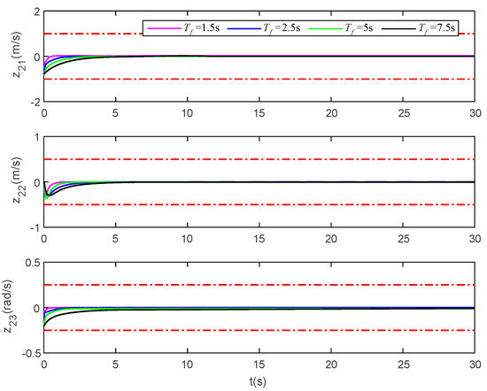
Figure 22. Velocity tracking error of the vessel under different settling time. (The upper and lower red dotted lines are error constraint boundaries).

Figure 21 and Figure 22 show the tracking error difference under different settling times $T_f=1.5 \mathrm{s}$, $T_f=2.5 \mathrm{s}$, $T_f=5 \mathrm{s}$ and $T_f=7.5 \mathrm{s}$. It can be seen that the tracking error of these two figures converges to near zero. Combined with the settling time $T_f=4 \mathrm{s}$, it can be seen that no matter what the settling time T_f is, the tracking error will satisfy the prescribed transient and steady-state performance. The simulation results further show that the method proposed in this manuscript is effective, and the full-state constraints and the performance of tracking error can be satisfied by the proposed method.

Figure 23 corresponds to the control force change curves under different settling time. It can be seen that the control curves of three-degree-of-freedom do not exceed their respective constraint ranges. When $T_f=1.5 \mathrm{s}$, $T_f=2.5 \mathrm{s}$, $T_f=5 \mathrm{s}$ and $T_f=7.5 \mathrm{s}$ the corresponding control force curve has the same general trend. Further, it can be seen that the transient requirement of error can be satisfied within the specified time by only adjusting T_f in the performance function without adjusting ${\mathit{K}}_i(i=1,2,3)$ again.

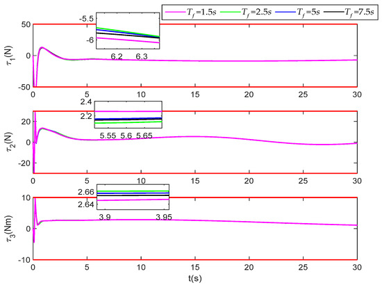
Figure 23. Control input under different settling time.

6. Discussion

The proposed finite time trajectory tracking prescribed performance control method is studied and analyzed, and its effectiveness is verified by simulations. The discussion results are as follows:

The error is transformed by the traditional prescribed performance control method, and then the controller is designed to satisfy the transient and steady-state requirements. In the process of designing the controller, we transform the constrained error into the unconstrained error, further construct the Laypunov function, and use the Laypunov direct method to solve the control law of each subsystem. Most of the performance functions used in the previous references are in infinite-time. However, considering the rapidity of the system in actual operation, the method of combining the performance function with finite-time is introduced, which effectively solves the convergence of the tracking error in finite-time and satisfies the requirements of transient and steady-state.

Previous references [10,11,12,13,14,15,16] only considered the transient and steady-state performance of errors, ignoring the constraint requirements of variables in the actual situation of the system. For dealing with constraint problems, the typical barrier Lyapunov function is an effective method, but how to combine a barrier Lyapunov function with the prescribed performance control is also a challenge, and the derivation of control law is relatively complex. Therefore, this manuscript considered to proceed directly from the perspective of parameter selection of performance function to avoid the inconvenience of derivation caused by introducing barrier Lyapunov function.

For system disturbances, [19,41] provide some effective methods, such as disturbance observer and active disturbance rejection control. Inspired by reference [19], the disturbance observer is designed based on the fractional order property. For integer order, fractional order can better describe some characteristics of disturbances changes.

In the entire control law design process, the matrix generalized inverse method is used to make the control law derivation more concise and save the previous scaling inequalities method.

In the future work, the full-state constraints form of the system is extended to a more general form, the time-varying constraints form, and further solve the prescribed performance trajectory tracking control of the surface vessel under the full-state time-varying constraints and input saturation of the system.

7. Conclusions

In this article an adaptive backstepping dynamic surface control method is proposed for the trajectory tracking problem of the surface vessel with full-state constraints and unknown environmental disturbances, and it is extended to the case where the system performance is required. Throughout the design process using smooth function matrix to approximate saturation function matrix, and the system model is augmented to construct auxiliary signals to obtain the required control input form. Finally, the finite-time performance function is constructed and combined with the Nussbuam function and the matrix generalized inverse, and then a finite-time full-state constraints controller is designed. In addition, the fractional order adaptive disturbance observer is designed to estimate the approximation error and external disturbance, and the robustness of the closed-loop system is improved. Through the proposed method, the vessel actual pose can be tracked to the desired pose, and the full-state constraints can be satisfied, and the system tracking error can satisfy the transient and steady-state performance in the finite time, and the control of the trajectory tracking control is realized. It is proved that all signals of the closed-loop system of the marine surface vessel are bounded. The simulation results verify the valid of the proposed method in this manuscript.

References

- Tee, K.P.; Ge, S.S.; Tay, E.H. Barrier Lyapunov functions for the control of output-constrained nonlinear systems. Automatica 2009, 45, 918–927. [Google Scholar] [CrossRef]
- Tee, K.P.; Ge, S.S.; Li, H.; Ren, B. Control of nonlinear systems with time-varying output constrains. Automatica 2011, 47, 2511–2516. [Google Scholar] [CrossRef]
- Ren, B.; Ge, S.S.; Tee, K.P.; Lee, T.H. Adaptive neural control for output feedback nonlinear systems using a barrier Lyapunov function. IEEE Trans. Neural Netw. 2010, 21, 1339–1345. [Google Scholar]
- Zhao, Z.; He, W.; Ge, S.S. Adaptive neural network control of a fully actuated surface vessel with multiple output constraints. IEEE Trans. Control. Syst. Technol. 2014, 22, 1536–1543. [Google Scholar]
- He, W.; Zhang, S.; Ge, S.S. Adaptive control of a flexible crane system with the boundary output constraint. IEEE Trans. Ind. Electron. 2014, 61, 4126–4133. [Google Scholar] [CrossRef]
- Yin, Z.; He, W.; Yang, C.G. Tracking control of a surface vessel with full-state constraints. Int. J. Syst. Sci. 2017, 48, 535–546. [Google Scholar] [CrossRef]
- Tang, Z.L.; Ge, S.S.; Tee, K.P.; He, W. Adaptive neural control for an uncertain robotic manipulator with joint space constraints. Int. J. Control. 2016, 89, 1428–1446. [Google Scholar] [CrossRef]
- Tang, Z.L.; Ge, S.S.; Tee, K.P.; He, W. Robust Adaptive Neural Tracking Control for a Class of Perturbed Uncertain Nonlinear Systems with State Constraints. IEEE Trans. Syst. Man Cybern. Syst. 2016, 46, 1618–1629. [Google Scholar] [CrossRef]
- Li, D.J.; Li, J.; Li, S. Adaptive control of nonlinear systems with full-state constraints using integral barrier Lyapunov functional. Neurocomputing 2016, 186, 90–96. [Google Scholar] [CrossRef]
- Bechlioulis, C.P.; Rovithakis, G.A. Prescribed performance adaptive control of SISO feedback linearizable systems with disturbance. In Proceedings of the 16th Mediterranean Conference on Control and Automation, Ajaccio, France, 25–27 June 2008. [Google Scholar]
- Bechlioulis, C.P.; Rovithakis, G.A. A low complexity global approximation-free control scheme with prescribed performance for unknown pure feedback systems. Automatica 2014, 50, 1217–1226. [Google Scholar] [CrossRef]
- Cao, C.; Hovakimyan, N. Design and analysis of IEEEa novel L1 adaptive control architecture with guaranteed transient performance. IEEE Trans. Autom. Control. 2008, 53, 586–591. [Google Scholar] [CrossRef]
- Cao, C.; Hovakimyan, N. Novel L1 neural network adaptive control architecture with guaranteed transient performance. IEEE Trans. Neural Netw. 2007, 18, 1160–1171. [Google Scholar] [CrossRef] [PubMed]
- Bechlioulis, C.P.; Rovithakis, G.A. Robust adaptive control of feedback linearizable MIMO nonlinear systems with prescribed performance. IEEE Trans. Autom. Control. 2008, 53, 2090–2099. [Google Scholar] [CrossRef]
- Wu, Z.; Lu, J.; Zhou, Q.; Shi, J.P. Modified adaptive neural dynamic surface control for morphing aircraft with input and output constraints. Nonlinear Dyn. 2016, 87, 2367–2383. [Google Scholar] [CrossRef]
- Wang, Y.H.; Wang, H.B.; Li, M.Y.; Wang, D.S.; Fu, M.Y. Adaptive fuzzy controller design for dynamic positioning ship integrating prescribed performance. Ocean Eng. 2020, 219, 107956. [Google Scholar] [CrossRef]
- Liu, Y.; Zhang, X.P.; Jiang, Y.W. Adaptive neural networks finite-time tracking control for non-strict feedback systems via prescribed performance. Inform. Sci. 2018, 468, 29–46. [Google Scholar] [CrossRef]
- Veksler, A.; Johansen, T.A.; Borrelli, F. Dynamic positioning with model predictive control. IEEE Trans. Control Syst. Technol. 2016, 24, 1340–1353. [Google Scholar] [CrossRef]
- Du, J.; Hu, X.; Krstić, M.; Sun, Y. Robust dynamic positioning of ships with disturbances under input saturation. Automatica 2016, 73, 207–214. [Google Scholar] [CrossRef]
- Zheng, Z.; Sun, L. Path following control for marine surface vessel with uncertainties and input saturation. Neurocomputing 2016, 177, 158–167. [Google Scholar] [CrossRef]
- Ma, J.; Ge, S.S.; Zheng, Z.; Hu, D. Adaptive NN control of a class of nonlinear systems with asymmetric saturation actuators. IEEE Trans. Neural Netw. Learn. Syst. 2015, 26, 1532–1538. [Google Scholar] [CrossRef]
- Chen, M.; Ge, S.S.; Ren, B. Adaptive tracking control of uncertain MIMO nonlinear systems with input constraints. Automatica 2011, 47, 452–465. [Google Scholar] [CrossRef]
- Zhang, Z.W.; Huang, Y.T.; Xie, L.H.; Zhu, B. Adaptive Trajectory Tracking Control of a Fully Actuated Surface Vessel With Asymmetrically Constrained Input and Output. IEEE Trans. Control Syst. Technol. 2018, 26, 1851–1859. [Google Scholar] [CrossRef]
- Yang, Y.; Chen, G.; Du, J.L. Robust adaptive NN-based output feedback control for a dynamic positioning ship using DSC approach. Sci. China Inf. Sci. 2014, 57, 1–13. [Google Scholar] [CrossRef][Green Version]
- Du, J.L.; Hu, X.; Liu, H.B.; Chen, C.L.P. Adaptive Robust Output Feedback Control for a Marine Dynamic Positioning System Based on High-Gain Observer. IEEE Trans. Neural Netw. Learn. Syst. 2015, 26, 2775–2786. [Google Scholar] [CrossRef] [PubMed]
- Vu, M.T.; Le, T.-H.; Thanh, H.L.N.N.; Huynh, T.-T.; Van, M.; Hoang, Q.-D.; Do, T.D. Robust Position Control of an Over-actuated Underwater Vehicle under Model Uncertainties and Ocean Current Effects Using Dynamic Sliding Mode Surface and Optimal Allocation Control. Sensors 2021, 21, 747. [Google Scholar] [CrossRef] [PubMed]
- Thanh, H.L.N.N.; Vu, M.T.; Mung, X.N.; Nguyen, N.P.; Phuong, N.T. Perturbation Observer-Based Robust Control Using a Multiple Sliding Surfaces for Nonlinear Systems with Influnences of Matched and Unmatched Uncertainties. Mathematics 2020, 8, 1371. [Google Scholar] [CrossRef]
- Wen, C.; Zhou, J.; Liu, Z.; Su, H. Robust adaptive control of uncertain nonlinear systems in the presence of input saturation and external disturbance. IEEE Trans. Autom Control. 2011, 56, 1672–1678. [Google Scholar] [CrossRef]
- Si, W.J.; Dong, X.D.; Yang, F.F. Adaptive neural prescribed performance control for a class of strict-feedback stochastic nonlinear systems with hysteresis input. Neurocomputing 2017, 251, 35–44. [Google Scholar] [CrossRef]
- Rakovic, S.V.; Kerrigan, E.C.; Kouramas, K.I.; Mayne, D.Q. Invariant approximations of the minimal robust positively invariant set. IEEE Trans. Autom. Control. 2005, 50, 406–410. [Google Scholar] [CrossRef]
- Mayne, D.Q.; Rawlings, J.B.; Rao, C.V.; Scokaert, P.O.M. Constrained model predictive control: Stability and optimality. Automatica 2000, 36, 789–814. [Google Scholar] [CrossRef]
- Wang, F.; Zhang, X.Y.; Chen, B.; Lin, C.; Li, X.H.; Zhang, J. Adaptive finite-time tracking control of switched nonlinear systems. Inform. Sci. 2017, 421, 126–135. [Google Scholar] [CrossRef]
- Hua, C.C.; Li, Y.F.; Guan, X.P. Finite/Fixed-time stabilization for nonlinear interconnected systems with dead-zone input. IEEE Trans. Autom. Control. 2017, 62, 2554–2560. [Google Scholar] [CrossRef]
- He, W.L.; Xu, C.R.; Han, Q.L.; Qian, F.; Lang, Z.Q. Finite-time L2 leader-follower consensus of networked Euler-Lagrange systems with external disturbances. IEEE Trans. Syst. Man Cybern. Syst. 2018, 48, 1920–1928. [Google Scholar] [CrossRef]
- Huang, X.Q.; Lin, W.; Yang, B. Global finite-time stabilization of a class of uncertain nonlinear systems. Automatica 2005, 41, 881–888. [Google Scholar] [CrossRef]
- Sun, Y.; Chen, B.; Lin, C.; Wang, H. Finite-Time Adaptive Control for a Class of Nonlinear Systems with Nonstrict Feedback Structure. IEEE Trans. Cybern. 2017, 48, 2774–2782. [Google Scholar] [CrossRef]
- Shen, Y.J.; Huang, Y.H. Uniformly observable and globally Lipschitzian nonlinear systems admit global finite-time observers. IEEE Trans. Autom. Control. 2009, 54, 2621–2625. [Google Scholar] [CrossRef]
- Podlubny, I. Caputo Fractional Derivative, Fractional Differential Equations; Academic Press: San Diego, CA, USA, 1999; Volume 2, pp. 32–51. [Google Scholar]
- Li, Y.; Chen, Y.; Podlubny, I. Mittag-Leffler stability of fractional order nonlinear dynamic system. Automatica 2009, 45, 1965–1969. [Google Scholar] [CrossRef]
- Yang, Y.; Du, J.L.; Liu, H.B.; Guo, C.; Abraham, A. A Trajectory Tracking Robust Controller of Surface Vessels with Disturbance Uncertainties. IEEE Trans. Control Syst. Technol. 2014, 22, 1511–1518. [Google Scholar] [CrossRef]
- Xue, W.; Bai, W.; Yang, S.; Song, K.; Huang, Y.; Xie, H. ADRC with Adaptive Extended State Observer and its Application to Air–Fuel Ratio Control in Gasoline Engines. IEEE Trans. Ind. Electron. 2015, 62, 5847–5857. [Google Scholar] [CrossRef]
Publisher’s Note: MDPI stays neutral with regard to jurisdictional claims in published maps and institutional affiliations. |
© 2021 by the authors. Licensee MDPI, Basel, Switzerland. This article is an open access article distributed under the terms and conditions of the Creative Commons Attribution (CC BY) license (https://creativecommons.org/licenses/by/4.0/).