Abstract
It is a well-known fact that the observed rise in the Arctic near-surface temperature is more than double the increase in global mean temperature. However, the entire scientific picture of the formation of the Arctic amplification has not yet taken final shape and the causes of this phenomenon are still being discussed within the scientific community. Some recent studies suggest that the atmospheric equator-to-pole transport of heat and moisture, and also radiative feedbacks, are among the possible reasons for the Arctic amplification. In this paper, we highlight and summarize some of our research related to assessing the response of climate in the Arctic to global warming and vice versa. Since extratropical transient eddies dominate the meridional transport of sensible and latent heat from low to high latitudes, we estimated the effect of climate change on meridional heat transport by means of the plane model of baroclinic instability. It has been shown that the heat transport from low and middle latitudes to the Arctic by large scale transient eddies increases by about 9% due to global warming, contributing to the polar amplification and thereby a decrease in the extent of the Arctic sea, which, in turn, is an important factor in the formation of the Arctic climate. The main radiative feedback mechanisms affecting the formation of the Arctic climate are also considered and discussed. It was emphasized that the influence of feedbacks depends on a season since the total feedback in the winter season is negative, while in the summer season, it is positive. Thus, further research is required to diminish the uncertainty regarding the character of various feedback mechanisms in the shaping of the Artic climate and, through that, in predicting the extent of Arctic sea ice.
1. Introduction
Among the current global issues that adversely affect the vital interests and fate of all of mankind, and require the consolidated efforts of all nation states for their solution, is climate change [1]. The results of paleoclimatic studies indicate that the climate of our planet has also changed in the past, when periods of warming were repeatedly replaced by periods of cooling [2]. These changes were caused by numerous internal and external factors with respect to the climate system, such as changes in the parameters of the orbit and axis of our planet, variations in the luminosity of the sun, the migration of continents and changes in their size and relief, changes in planetary albedo, changes in transparency and the atmospheric gas and aerosol composition, etc. However, current climate change has two essential distinctive features. First, the quickness and extent of changes in the Earth’s climate system (ECS) are unprecedented. According to the US NOAA (National Oceanic and Atmospheric Administration) summary report [3], since 1880, the global mean near-surface air temperature (GMST) has risen by ~0.07 °C every 10 years. Meanwhile at the turn of the millennium, the growth rate of GMST reached 0.17 °C per decade, meaning that it more than doubled. Secondly, current global warming is “man-made” since its main cause lies in human activity. According to the IPCC (Intergovernmental Panel on Climate Change) Fifth Assessment Report [4], “it is extremely likely that more than half of the observed increase in global average surface temperature from 1951 to 2010 was caused by the anthropogenic increase in greenhouse gas (GHG) concentrations and other anthropogenic forcings together”. It is known that one of the most significant signs of anthropogenic activities is a dramatic increase in the atmospheric carbon dioxide (CO2) content, whose contribution to global warming is about 65%. Over the past million years, the concentration of atmospheric CO2 has varied from 0.018 to 0.028%. Since the beginning of the industrial revolution (~1850), as a consequence of the burning of fossil fuels, the concentration of CO2 in the atmosphere has constantly increased and, by 2019, reached 0.041% [5].
In general, there is a scientific and political consensus in the assessment of trends in climate change and the reasons giving rise to this change, which is enshrined in the IPCC report [4] and a recently published report [6] that has been signed by over 11 thousand scientists. Presently, the confidence of the available estimates regarding the determining role of the anthropogenic factor in modern climate change (towards warming) is 99.99995% reaching a “five-sigma” level of certainty, which corresponds to the so-called “gold standard” [7]. Changes in the climate system can be identified using some indicators, which are the observable and measurable characteristics of the climate system that allow us to assess its state. The World Meteorological Organization (WMO), at a meeting held on 3 February 2017, identified seven key global indicators of climate change, calculated on the basis of 54 variables provided by the GCOS (Global Climate Observing System) [8]. The key global indicators of climate change include:
- Globally averaged annual near-surface temperature;
- Heat content of the global ocean;
- Concentration of CO2 in the atmosphere;
- Globally averaged sea level;
- Ocean acidification;
- Sea ice extent in the Arctic and Antarctic, state of glaciers; and
- Global precipitation.
In the opinion of the WMO experts, these indicators contain crucial information for the trend and rate of the ongoing climate change and, therefore, fairly well characterize the observable global warming. When studying the essential features of Arctic climate change, one can use additional indicators that characterize the Arctic climate system. For instance, in [9,10], the following nine observational indicators were used to examine the status of the climate and ecosystem at high latitudes:
- Air temperature after NCEP/NCAR reanalysis data (North Hemisphere annual temperature, Arctic warm season air temperature, Arctic annual air temperature, and Arctic cold season air temperature);
- Average permafrost temperatures in some areas of Alaska;
- Precipitation data after NCEP/NCAR reanalysis (Arctic October to May precipitation, Arctic June to September precipitation, and Arctic annual precipitation);
- Arctic river discharge totals from Eurasian and North American regions;
- Pan-Arctic tundra maximum Normalized Difference Vegetation Index (NDVI) for elevations below 300 m, occurring in late July or early August, averaged over Arctic tundra;
- North American burned area (the sum of Alaska and Canada’s Northwest Territories, respectively);
- Spring snow cover duration of Arctic land area, excluding Greenland;
- September Arctic sea ice extent;
- Regional glacier mass balance standardized anomalies.
In this regard, it should be emphasized that the Arctic sea ice plays the role of one of the most important indicators of trends in high latitude climate change [11,12,13,14,15,16,17,18,19]. However, the Arctic sea ice extent caused by natural and human-induced factors, in turn, affects the high latitude climate and northern hemispheric climate via feedbacks that, unfortunately, are not completely understood.
Interestingly, the rise in the Arctic near-surface temperature is more than double the increase in global mean temperature. This phenomenon is called “Arctic amplification” (e.g., [20,21,22,23,24,25,26,27]). It should be noted that the entire scientific picture of the formation of the Arctic amplification has not yet taken final shape and the causes of this phenomenon are still being discussed within the scientific community. Many recent studies (see [17,18,19,28,29,30,31,32] and references therein) show that the possible causes of Arctic amplification include meridional (equator-to-pole) sensible and latent heat transport in the atmosphere, the decrease in sea ice extent, feedbacks of water vapor, cloud, lapse rate, surface albedo, and Planck feedback. It is clear that many of these physical processes are interdependent. Therefore, the overall picture of the formation of the Arctic climate is quite complex and multifaceted in terms of its full range of details and manifestations. This determines the need for further studies of the physical mechanisms of the formation of the Arctic climate, and estimation of their relative importance.
This paper intends to highlight and summarize some results of our research related to the estimation of the response of Arctic climate change to global warming, with a focus on the role that non-stationary large scale atmospheric eddies play in the meridional equator-to-pole transport of sensible and latent heat.
2. Meridional Equator-to-Pole Sensible and Latent Heat Transport in a Changing Climate
2.1. Meridional Heat and Moisture Transport: Linear Approximation
The naturally-occurring climate processes draw energy mainly from the Sun [33,34,35]. Meanwhile, climates in different geographical areas of the world differ from each other due to a number of factors, but primarily because of fluctuations in the average annual amount of radiation from the Sun that reaches the top of the atmosphere (TOA) [36]. Since insolation (i.e., the amount of downward shortwave radiation from the Sun incident on a plane surface at the TOA) is most dependent on latitude, climatic conditions, on average, also considerably vary with latitude. That is why the polar climate is so different from the tropical and mid-latitude climates. It is obvious that the horizontal inhomogeneity of the atmosphere and the surface of our planet perturbs the latitudinal zoning in the distributions of reflected and absorbed radiation, but these disturbances are not strong enough to perturb the approximate climate latitudinal zonation [36]. The Arctic is characterized by a relatively small amount of incoming solar radiation compared to other parts of the planet. Moreover, during the polar night, the Arctic does not receive solar energy at all. At the same time, during the polar day, a relatively small amount of solar energy reaches the Arctic because of the low angle of incoming rays. The energy balance in the Arctic is also substantially affected by the presence of sea ice cover with a high albedo. Thus, one of the distinctive particularities of the Arctic is that its climate system is characterized by net energy losses for most of the year [37]. Another important characteristic of the Arctic climate is that the annually averaged near-surface temperature increase in the Arctic region tangibly exceeds the rate of warming in other parts of the world [20,27]. An obvious manifestation of Arctic warming is, among others, a decrease in the sea ice extent during the summer period [17]. As shown in [17,18], the correlation coefficient between changes in the Arctic surface temperature in the summer season and the sea ice in September is about −0.93.
The poleward (meridional) energy transport, mainly by the atmosphere, serves as a compensatory mechanism of the existing radiative imbalance in the Arctic (e.g., [38,39]). The beginning of the research on the transport of energy to polar regions was largely stimulated by the studies of Budyko [40] and Sellers [41], in which energy balance climate models (EBM) were used with parameterized heat transport into high latitudes. Then, in numerous studies, various types of observations, including satellite observations and reanalysis, were used to explore the essential features of meridional energy transport from low to high latitudes (e.g., [18,27,42,43,44,45,46,47,48,49] and references therein). However, the analysis of observation-based studies and research conducted using climate models shows a high uncertainty in assessing the role of various physical processes in the formation of climate in polar areas. In particular, the role of meridional energy transport in the Arctic amplification remains controversial, and requires further development.
Generally, to analyze the energy transport in the atmosphere, the variable known as moist static energy is used, which the per unit mass of moist air is defined as follows:
where the sum of enthalpy and potential energy represents the dry static energy (where is the temperature, is the specific heat of dry air at constant pressure, is the gravitational acceleration, and is the geopotential height). The term is the energy of latent heat, where is the latent heat released per unit mass when the atmospheric water vapor condensed or the cloud droplets evaporated, and is the specific humidity.
The energy budget of a given column of the atmosphere in terms of the rate of change over time in moist static energy represents the sum of net radiation at the TOA, , the net heat flux near the surface, , and vertically integrated horizontal energy flux divergence, [44]. The horizontal energy flux divergence integrated between the surface and the TOA is calculated as follows [50]:
In this equation, is the vector of horizontal wind and is the vertically integrated horizontal energy flux, defined as follows:
where and are, respectively, the pressure and the surface pressure. The divergence theorem allows the computation of as the following line integral [50]:
where is the area of the region, which is bounded by the curve , and is a unit vector normal to the boundary. In a similar way, one can consider not only the transport of moist static energy in general, but also its individual components, such as sensible heat and/or latent heat.
The effect of the atmospheric meridional transport of sensible and latent heat on amplified warming and temperature variability in the Arctic has been intensively and systematically analyzed and explored over the years at the Arctic and Antarctic Research Center (AARI) [17,18,25,48,51,52], which is based in St. Petersburg, Russia. By analyzing the meridional heat and moisture transport into the high latitudes (north of ), one can neglect the potential energy term in (1), since the main purpose of the research was to assess the effect of both sensible and latent heat transport on temperature changes, but not on energy in general, in the region that is northward of . Thus, the domain of interest is the north polar cap, bouded by a fixed line of latitude that is . In this case, the normal velocity is the meridional wind component v.
ERA-Interim reanalysis data [53] were used to calculate monthly average meridional atmospheric heat and moisture fluxes, with spacing along the 70th parallel north, on 20 isobaric levels, ranging from 1000 to 50 hPa with a 50-hPa resolution. The results obtained show that both sensible and latent low-tropospheric (between the surface and the geopotential height of 750 hPa) heat fluxes are the main cause of more than 50% of surface temperature changes in the Arctic winter season. However, in the summer season, radiation processes, primarily downward longwave radiation, are the main driver of warming. Similar results were obtained from simulations produced by CMIP5 global climate models.
From a climatological perspective, the vertically integrated northward sensible and latent heat transport averaged over time and around a latitude circle is of interest, which represents the sum of three major components (e.g., [34,43]):
In the above equation, the overbar denotes the average time and the prime is the deviation from the mean time; the square brackets and asterisks denote, respectively, zonal mean and deviation from it. In the right-hand side of (5), the first term is the contribution from the global mean meridional circulation; the second and third terms are, respectively, the contributions from stationary and transient eddies.
Meanwhile, in the equator-to-pole heat and moisture transport, a key role is played by large-scale extratropical transient eddies (e.g., [54]). As confirmed by observation datasets and results of numerical simulations with complex climate models, extratropical transient eddies (weather systems), dominate meridional transport of sensible and latent heat from tropics to polar regions. The main physical mechanism of the generation of extratropical cyclonic eddies is the atmospheric baroclinic instability on the rotated Earth [55]. In this case, the mean available potential energy (MAPE) is the main source of energy for the growing atmospheric perturbations. Note that MAPE is determined primarily by the tropospheric meridional temperature gradient (MTG) [56]. The increments of unstable perturbations depend not only on the MTG, but also on the atmospheric static stability [57]. It is very important that climate change affects both MTG and static stability (e.g., [58,59,60,61]), and thus, the large-scale eddy intensity at middle and high latitudes. Let us consider how climate change affects the development of baroclinic instability and, as a consequence, the meridional heat and moisture transport by large-scale eddies in the atmosphere. Conditionally, the life cycle of atmospheric baroclinic instability can be divided into three basic stages: (1) the exponential growth of initially small perturbations; (2) the formation of large-scale eddies; and (3) the dissipation of eddies. To study the initial stage of baroclinic instability, linearized dynamics equations are usually applied. In this case, the baroclinic instability is considered as an eigenvalue problem that is usually solved using the perturbation method, which admits a plane-wave solution. Then, it can be shown that the meridional heat flux due to transient eddies depends exponentially on the increments of unstable perturbations [62]. Let us explain this in more detail. In accordance with the perturbation method, any dependent atmospheric variable is represented as the sum of a reference state and a sufficiently small perturbation , so that :
where is a reference state function, and is a sufficiently small (infinitesimal) perturbation such that , in which x and y are eastward and northward Cartesian coordinates; pressure p is used as vertical coordinate; t is time. Substituting (6) into the nonlinear equations of atmospheric dynamics that are used to examine baroclinic instability (usually, these equations include at least the equations of motion, the continuity equation and the equation of thermodynamics [63]) and then neglecting the terms of second order, one can derive the linear perturbed differential equations. These linear equations, as was mentioned above, admit plane-wave solutions. Considering the model of baroclinic instability [63,64], we can seek the normal mode (plane-wave) solution:
where is the amplitude of perturbation, which depends on p only; is a zonal wavenumber (where is the radius of the Earth, is the latitude, and is the wavelength); c is a perturbation’s phase velocity.
Substituting the normal mode solution (7) into the linearized model equations, one can derive the system of algebraic equations that can be solved analytically with respect to phase velocity c. The increments of unstable waves, represented by , are defined as , where is the imaginary part of the phase velocity. For the plane (Phillips) model, which is the classic model of baroclinic instability, the growth rate is calculated as follows [57,62]:
where is the parameter related to static stability, in which is the reference value of Coriolis parameter calculated by the formula , is the angular velocity of our planet and is the reference latitude, ; is the thermal wind characterizing MTG, where and are the wind velocity at, respectively, the 250 hPa and 750 hPa pressure levels.
Transient extratropical large-scale atmospheric eddies are wave phenomena that have typical space scales of zonal wavenumbers 5–7. Note that eddies with higher zonal wavenumbers “have the right to life” with fastest growth rates and their energy is concentrated in the lower troposphere [63,65]. Let us define as a wavelength and as a wavenumber of unstable mode, then the following can be obtained:
Expressions (9)–(11) can be rewritten as follows:
were , and are the absolute values of complex variables , and , and , and are their arguments; is the real part of the complex phase velocity.
The meridional heat and moisture fluxes averaged over one period of the unstable wave, , can be calculated by the following equations [63]:
Substituting (12)–(14) in Equations (15) and (16), and then applying periodic boundary conditions, one can derive the following formulas for fluxes and :
Equations (17) and (18) show that the meridional heat and moisture transport is strongly affected by the increment of unstable waves, which depends, firstly, on wavenumber (wavelength) of the unstable wave k () and, secondly, on the imaginary part of the phase velocity , which, in turn, is dependent on the atmospheric static stability and the vertical wind shear [64].
2.2. Estimation of the Climate Change Impact on the Characteristics of Large-Scale Atmospheric Eddies
Let us consider how global warming affects the wavelength of the unstable baroclinic wave or, in other words, the horizontal size of large-scale atmospheric eddies. The typical horizontal size of these eddies is usually estimated by the first internal Rossby radius of deformation , defined as follows [66]:
where N is the buoyancy frequency; f is the Coriolis parameter; H is the height of homogeneous atmosphere; is the vertical temperature lapse rate, and is the dry adiabatic lapse rate. For characteristic values of variables, namely , ; , we have .
To estimate the effect of climate change on we can use the following sensitivity coefficient:
However, based on this equation, it is not so easy to draw an unambiguous conclusion on how climate change affects the horizontal size of atmospheric cyclonic eddies. In the atmosphere, the typical value of the “standard” large-scale lapse-rate is less than the dry adiabatic lapse rate . In addition, the value of is small. Therefore, depending on how the lapse rate behaves under the influence of climate change, two scenarios are possible: (1) and (2) , respectively. To clarify this situation, we introduce two partial sensitivity coefficients:
Equation (21) shows that an infinitesimal change in temperature causes a partial change in the Rossby deformation radius of . Since the reference value of the annual global mean surface temperature (GMST) is about 288 K, we can find that an increase in surface temperature of 1 K (i.e., ) results in an increase in the characteristic size of eddies of only 0.2%. Proceeding in the same way, from Equation (22), we derive the following formula for estimating the effect of a sufficiently small variation of the temperature lapse rate on a fractional variation in the Rossby radius of deformation: . Since the reference value of the tropospheric is we find that if , then the characteristic size of eddies decreases by 15%. Unfortunately, there is no a priori information on the relationship between temperature growth and change in the lapse rate. Consequently, estimating the total sensitivity coefficient (20) is not a simple task. In general, in order to estimate the effect of climate change on the size of atmospheric eddies, we should take into account atmospheric moisture. To this end, the so-called “effective” lapse rate defined by should be used in calculations, where is the moist adiabatic vertical temperature gradient and is a cloud fraction. The value of the total sensitivity coefficient , obtained from the NCEP/NCAR reanalysis datasets, is , while from the climate modeling results, the values of and are obtained, respectively, for dry and moist atmospheres [66]. Thus, climate change insignificantly affects the size of cyclonic eddies in the atmosphere. Climate change can also affect the frequency of occurrence of eddies. Applying the sensitivity coefficient (here n is the annual average number of cyclonic eddies, one can estimate as a first approximation the impact of climate change on n. The value of the coefficient , obtained from the NCEP/NCAR reanalysis datasets, is , while the value obtained from the results of climate modeling for dry (moist) atmosphere is () [66]. Thus, climate change results in a decrease in by about 3–4%.
There is no doubt that the estimates considered should be approached with caution, since they were obtained under simplified assumptions and, therefore, have a certain degree of uncertainty. However, these estimates provide some quantitative insight into how global warming can influence both the size and number of atmospheric transient eddies.
2.3. The Impact of Climate Change on the Increment of Large-Scale Baroclinic Unstable Waves
As discussed in Section 2.1, for the plane baroclinic instability model, the increments of unstable waves given by Equation (8) depend on the static stability of the atmosphere and wind shear in the vertical direction that is uniquely related to MTG. For the current climate, the following reference values of the atmospheric static stability and thermal wind shear can be considered [63]: and . The effective static stability parameter calculated for the moist atmosphere is about . These are the so-called base parameter values.
Increments of unstable waves, depending on zonal wavenumber, are shown in Figure 1. These increments were calculated with base parameter values for the “dry” and “moist” models. Accounting for atmospheric moisture, as we can see in Figure 1, has two clear effects. First, the spectrum of unstable waves expands quite tangibly, and this expansion extends mainly towards short waves. Second, the increments of unstable waves increase significantly. For instance, the increment of the most unstable wave increases from 0.45 to 0.68 day−1.
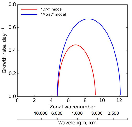
Figure 1.
Increments of unstable baroclinic waves for “dry” and “moist” plane models.
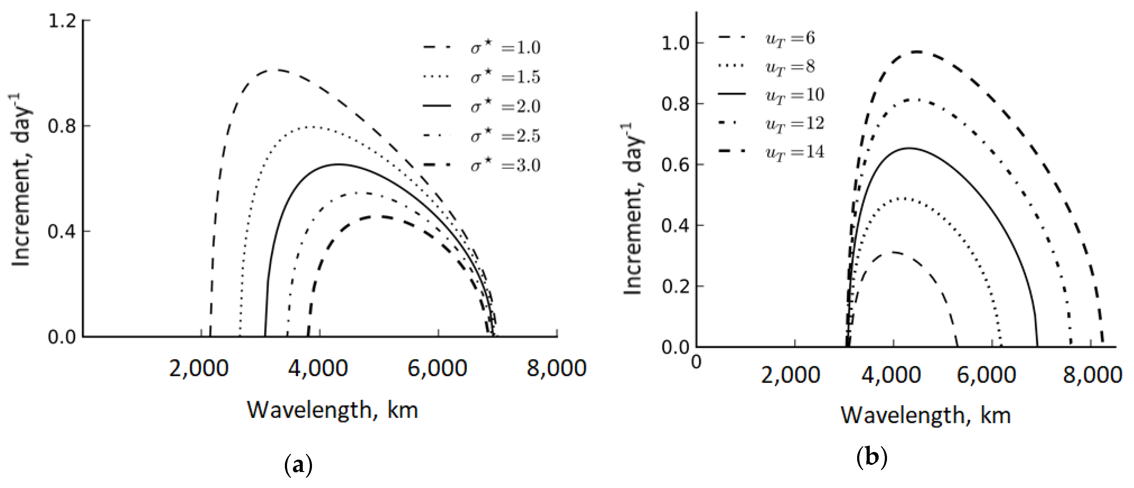
Since climate change affects both static stability and MTG [67], we calculated, for reference, the increments of unstable waves for different values of the parameters and . Figure 2 illustrates the results obtained using the “dry” model.
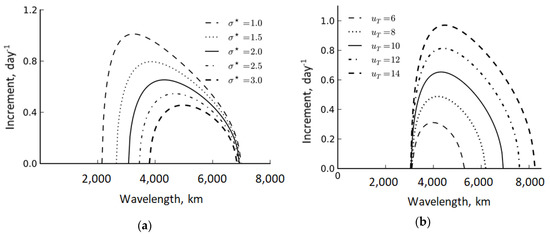
Figure 2.
Increments of unstable baroclinic waves for different static stability parameters (a) and vertical wind shear (b).
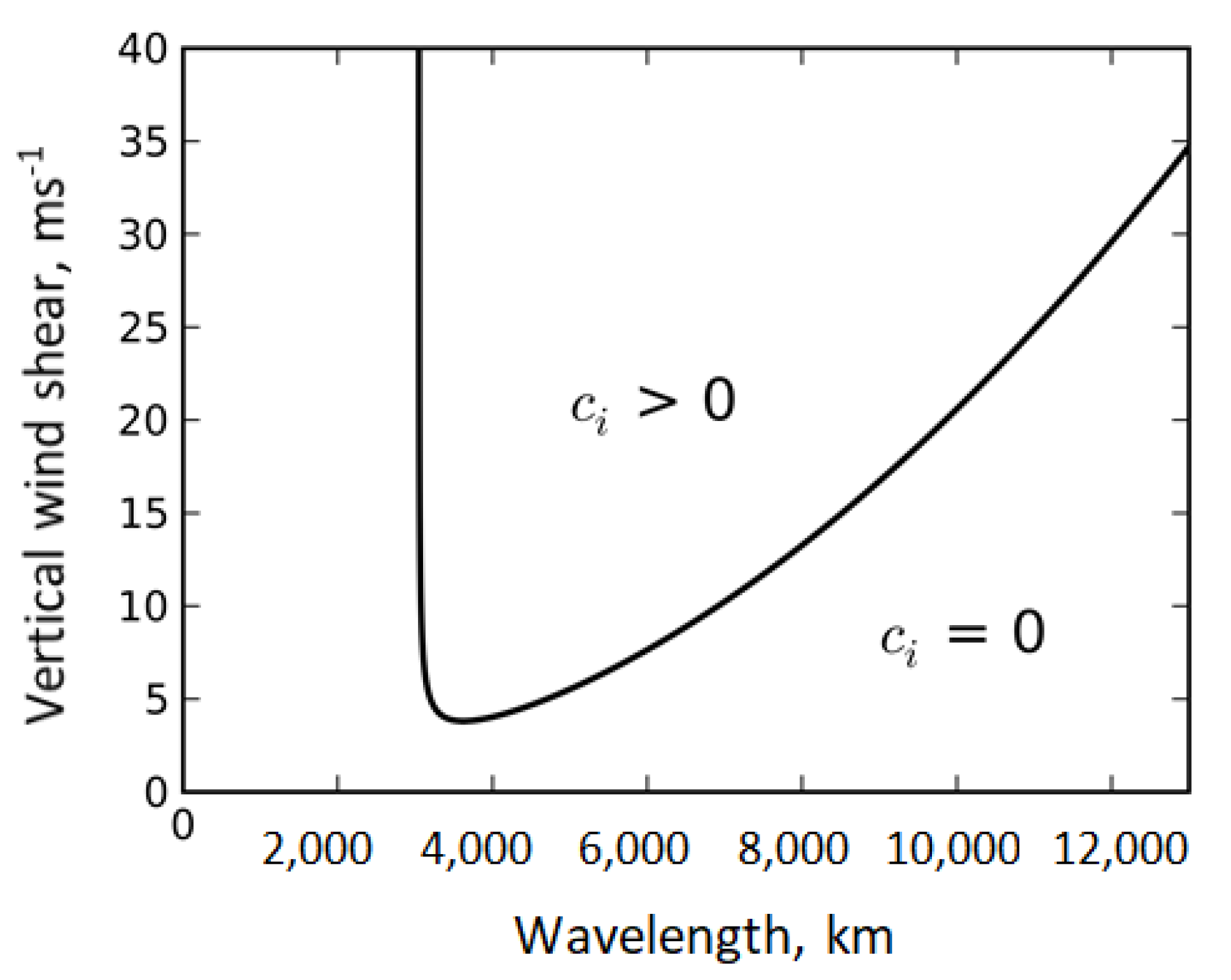
If we set the discriminant in (8) equal to zero, we can find, first, the marginal stability curve, which will separate unstable atmospheric waves from stable ones (see Figure 3), and second, the shortwave cut-off and longwave cut-off . Note that the wavelength of an unstable wave satisfies the condition . For the “dry” (“moist”) model, the cut-off is 3085 km (2333 km) for short waves, and 5945 km (6015 km) for long waves.
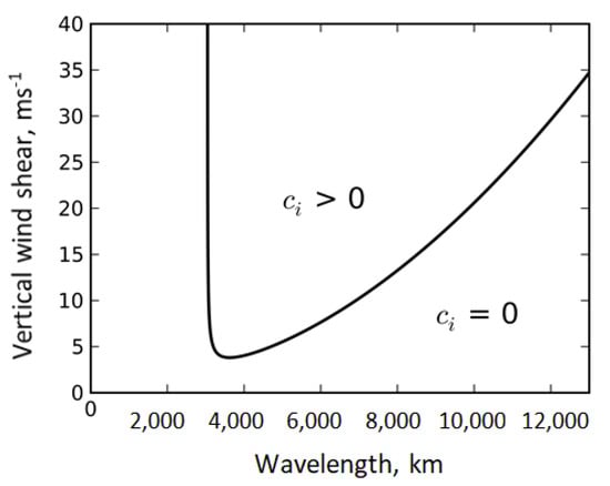
Figure 3.
Marginal stability curve.
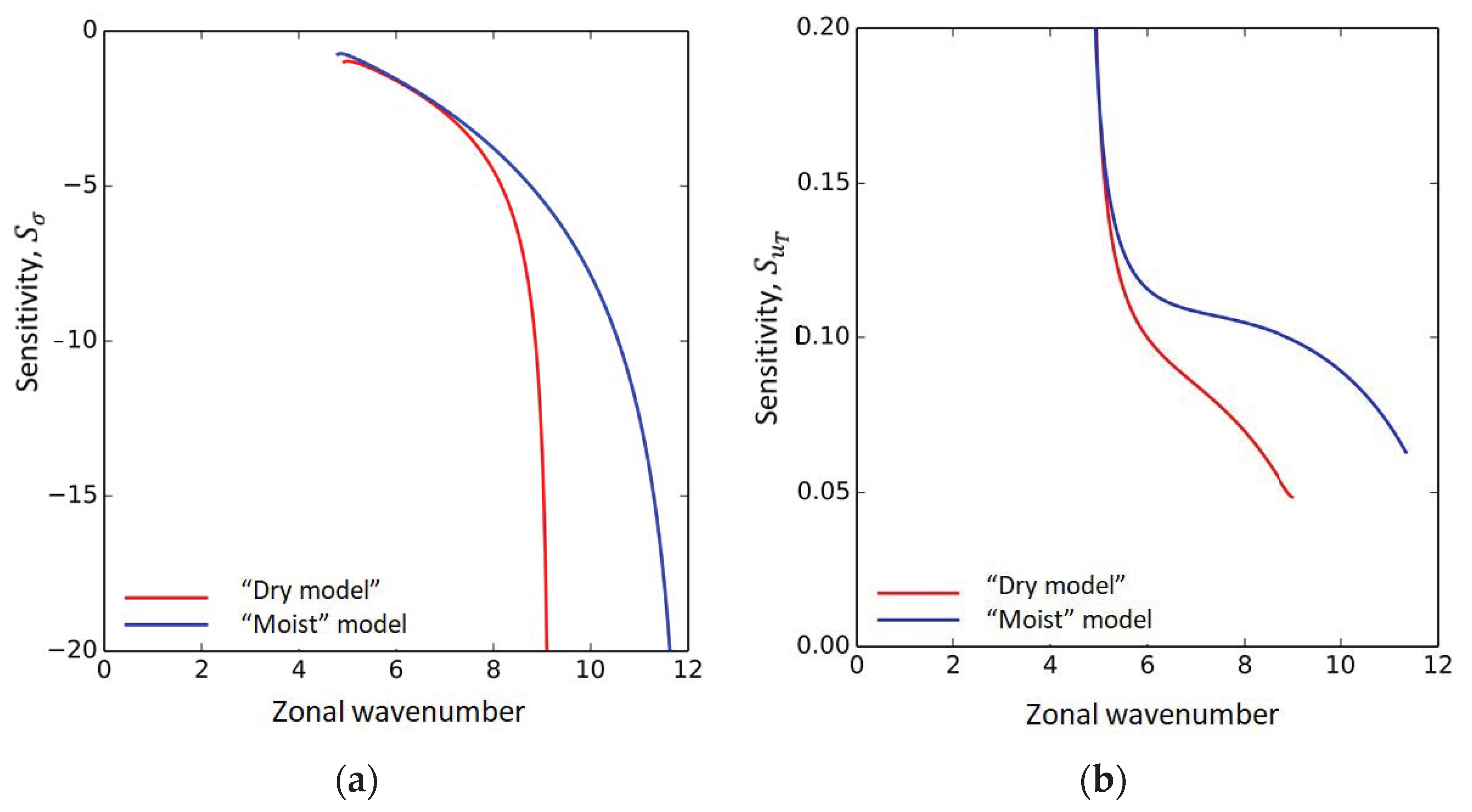
To assess the impact of climate change on the increments of unstable waves, we use conventional sensitivity analysis, which involves the calculation of the corresponding sensitivity functions [68]. The sensitivity functions and , with respect to parameters and , allow the determination of the effect of small perturbations in and on the growth rates of unstable waves. The sensitivity functions represented as partial derivatives of the instability increment , with respect to and , are as follows [62]:
The graphs of sensitivity functions and , calculated for dry and moist atmosphere, are presented in Figure 4. Since the modulus of exponentially increases with the decreasing of the wavelength, the shorter the wavelength, the greater the effect of variations in on the increment of an unstable wave. Short waves also turn out to be more sensitive to changes in MTG then long waves. Atmospheric moisture increases the sensitivity of increments of unstable waves to both and MTG. The effect of moisture is also more significant in the shortwave domain of the spectrum.
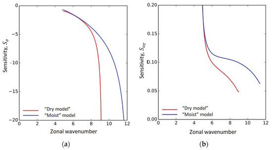
Figure 4.
Sensitivity functions (a) and (b) for “dry” and “moist” models.
By varying both and , one can assess the impact of climate change on as follows: and In order to conduct this assessment, the climate change scenario should first be defined. Based on the observational data [59], it was found that due to global warming, the average temperature lapse rate has, over the last few decades, decreased from 6.5 to 6.3 . As a result, the dry static stability parameter increased by about 0.7% relative to the base value . However, it is very remarkable that the effective static stability parameter changed in the opposite direction: it decreased by more than 5.4%. Thus, if, in the models, we neglect the moisture of the atmosphere, then we can obtain completely different and even opposite results in the estimation of the impacts of global warming.
Calculations show that in a dry atmosphere, the most unstable wave has a length of about 4130 km. Due to climate change, its growth rate decreases by day−1, which is only 0.7% of the reference value of 0.45 day−1. Meanwhile, in a moist atmosphere, the most unstable wavelength is ~3385 km. Due to climate change, its increment increases by about day−1 (~3.5% of the reference value of 0.68 day−1). Changes in the growth rate cause changes in the poleward transport of sensible and latent heat. Using Equations (17) and (18), this effect can be estimated. In a dry atmosphere, the meridional transport of heat and moisture decreases by only about 0.5% compared to the base case scenario, while in the moist atmosphere, the meridional heat and moisture transports increases by about 5%. These estimates were obtained for the most unstable baroclinic wave.
Let us now consider how the change in MTG caused by global warming can affect the behavior of unstable baroclinic waves. As shown in [62], global warming causes changes in MTG, which lead to corresponding changes in the parameter such that . Using sensitivity function , one can estimate the impact of global warming on caused only by . Calculations show that the increments of unstable waves in a dry atmosphere increase by ~ day−1 (almost 4% of the reference value), and in a moist atmosphere by ~ day−1 (about 3.1% of the reference value). In addition, meridional heat and moisture transport, as estimated using Equations (17) and (18), increase by about 4.2% for both dry and moist atmosphere. Thus, using the conventional sensitivity approach, we obtain that the increase in poleward latent and sensible heat transport caused by the change in the effective static stability is about 5%, while the change in the MTG results in an increase in the equator-to-pole heat flux of about 4%. After summarizing the changes in heat transport relative to global warming, the total increase in the poleward heat transport is about 9% relative to the base case scenario.
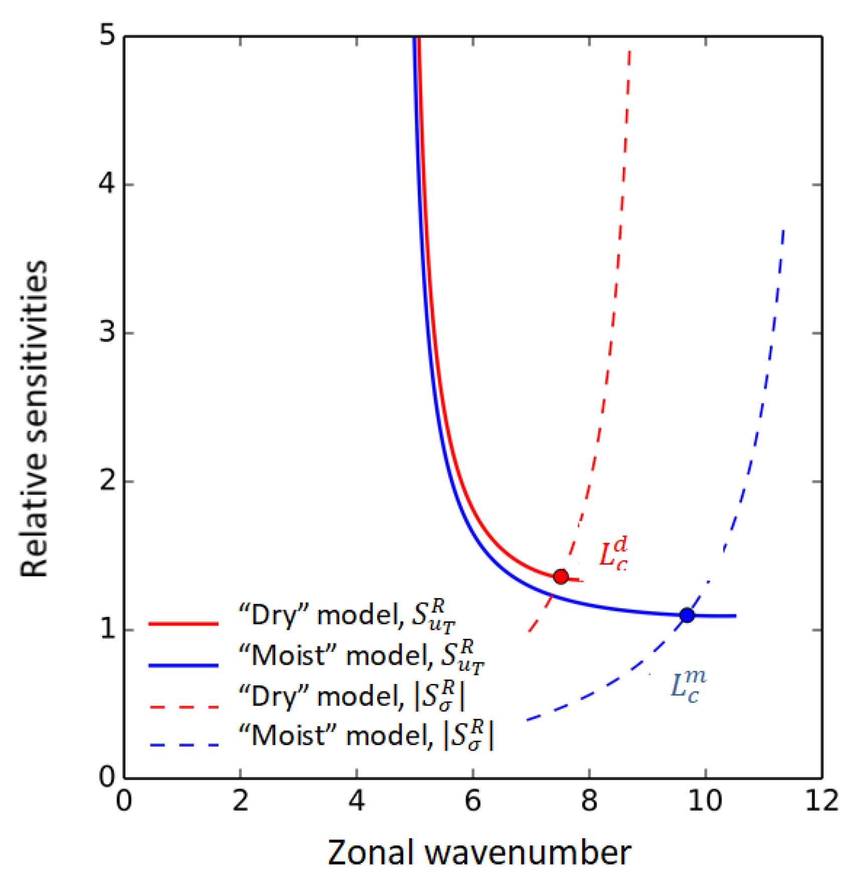
It is useful, as well, to assess the relative influence of and on the increments of unstable waves in order to rank them according to the degree of their influence on the development of baroclinic instability. For this purpose, the relative sensitivity functions can be used, which are defined as , where (, ). As shown in Figure 5, there is a critical wavelength which splits the spectrum of unstable waves into two domains. One of them corresponds to waves, the development of which is most significantly influenced by static stability (), while the development of waves with is more affected by MTG. Importantly, the atmospheric moisture significantly changes the value of . For the “dry” (“moist”) model, the is 3800 (2900) km.
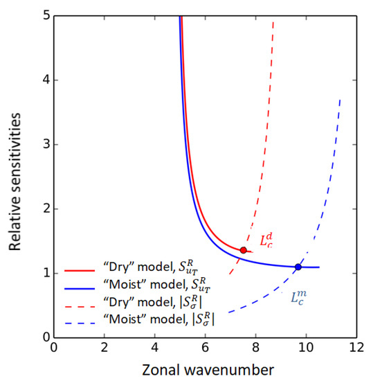
Figure 5.
Relative sensitivity functions for “dry” and “moist” models.
3. Climate Feedbacks in the Arctic
Climate feedback mechanisms have an important place in the shaping of climatic conditions around the world and in its various parts, including the Arctic, since feedbacks amplify or reduce the response of the climate system to radiative forcing [31,69]. Typically, climate system feedbacks are explored by analyzing the global mean energy imbalance at TOA, , caused by natural and/or anthropogenic radiative perturbation . When analyzing climate feedbacks, the following basic assumption is usually used: changes in surface temperature , caused by radiative perturbation , generate proportional changes in the radiative flux at TOA, namely, , where with units of is the feedback parameter (we assume the downward fluxes are considered positive). Thus, feedback parameter given by the variation in (downward) net radiative flux at TOA for a given variation in surface temperature quantifies a particular feedback mechanism in the climate system.
To analyze various feedback loops in the climate system, we should, first, introduce a so-called reference dynamical system. In climate studies, the reference system describes only Planck feedback [70], which represents variations in outgoing infrared radiation at TOA due to changes in surface temperature. Plank feedback being the most basic type of feedback in the climate system is negative. This feedback is described by the Stefan–Boltzmann law. For the reference system, the Planck feedback parameter that links the surface temperature variation to the variation in the radiation balance at TOA is of (where is the emissivity of the Earth’s system, the constant is the Stefan–Boltzmann constant, and is the GMST). Thus, as the surface temperature rises, the emission of long-wave infrared radiation into space will also increase, thereby producing a cooling effect. It is clear that in the Arctic, the climate system’s response to radiative forcing, via the Planck mechanism, is less than in the tropics, since the outgoing long-wave radiation at TOA is linearly dependent on surface temperature to the fourth power. Each climate feedback mechanism is characterized by a specific feedback parameter), where is the number of feedback loops taken into consideration. The net feedback is approximately estimated as follows: .
In the climate system, the change in temperature due to global warming is vertically non-uniform, depending on the geographical region. As a result, the temperature lapse rate changes non-identically, in different parts of the world that are experiencing climatic effects, via the so-called lapse rate feedback . Thus, lapse rate feedback is solely caused by variations in the vertical temperature distribution. In response to an increase in the concentration of greenhouse gases, at low latitudes, there is increased warming in the upper troposphere, leading to an increase in the amount of outgoing infrared radiation compared to a uniform vertical temperature change, thereby producing a negative radiative feedback or, in other words, some cooling of the Earth system [71,72]. A slightly different picture is observed in the Arctic regions, where enhanced warming occurs mainly in the lower troposphere, while the upper troposphere practically does not warm up, resulting in a decrease in outgoing long-wave radiation causing further warming [71]. Therefore, at high latitudes, the lapse rate feedback is positive [71].
Climate change facilitates intensification of the global hydrological cycle since, with increases in the atmospheric temperature, the amount of water that has evaporated from the ocean’s surface and other reservoirs to the atmosphere and, therefore, the total atmospheric content of water vapor will increase as well. According to Clausius–Clapeyron relation, if the air temperature rises, then the saturated pressure of water vapor increases by about seven per cent per Kelvin degree, while the relative humidity remains almost constant. Thus, the atmospheric moisture content increases during global warming. Satellite observations are in very good agreement with these theoretical estimates. Meanwhile, water vapor is a highly efficient greenhouse gas, which traps the outgoing infrared radiation. Consequently, the greenhouse effect is enhanced by the additional large amount of water vapor released to the atmosphere due to climate change. This positive water vapor feedback is more significant at low latitudes than in the Arctic, but its role at high latitudes is not so weak as to be neglected [30].
The next feedback mechanism that is very important in the Arctic is ice–albedo feedback, which is associated with sea ice melting with warming. Due to the rise in surface temperature at high latitudes, the area of the ice cover is reduced and replaced by a water surface. These processes lead to a decrease in the regional surface albedo and an increase in the amount of solar energy that is absorbed by the Earth’s surface, resulting in further warming and, therefore, shrinking of the sea ice area. Thus, the ice–albedo feedback is positive in the Arctic.
The most uncertain feedback mechanism in the climate system is cloud feedback. According to the IPCC Fifth Assessment Report [4], “… changes in high-level cloud altitude, effects of hydrological cycle and storm track changes on cloud systems, changes in low-level cloud amount, microphysically induced opacity (optical depth) changes and changes in high-latitude clouds.” With regard of the cloud feedback mechanism, the report states the following: “The sign of the net radiative feedback due to all cloud types is less certain but likely positive.” In the Artic, cloud feedback is positive in non-summer time, and close to zero in the summer season [30]. This is due to the fact that a decrease in the ice cover extent (in non-summer time) results in an increase in cloudiness and, as a consequence, an increase in downward infrared radiation, which leads to further melting of sea ice. However, with climate warming, the portion of liquid water in mixed-phase clouds rises, contributing to an increase in cloud albedo and, therefore, a greater reflection of shortwave solar radiation; this leads to a decrease in warming (negative feedback).
As mentioned earlier, the total radiative feedback in the first approximation can be estimated as a combination of all radiative feedback mechanisms, which, in turn, are controlled by one or several climate variables. As shown in [72], the total feedback at high latitudes is strongly negative in the cold seasons of the year () by virtue of the predominance of Planck feedback. However, during the summer, the total feedback is positive (). These estimates were derived from simulations with 13 climate models with abruptly quadrupling carbon dioxide concentrations.
In this paper, we focused on atmospheric feedbacks only. There is no doubt that ocean dynamics play an important role in the shaping of the Arctic climate and the extent of Arctic sea ice (e.g., [73]). However, the following is mentioned in [74]: “To date, no clear consensus regarding the detailed impact of ocean heat transport on Arctic sea ice exists”. Therefore, this problem requires specific consideration.
4. Discussion and Concluding Remarks
The Arctic warming of recent decades, characterized by the so-called Arctic amplification that is characterized by significantly rapid increases in surface temperature compared to global temperature changes, was followed by a reduction in the sea ice extent. Thus, the sea ice extent in the Arctic represents one of the key indicators of worldwide climate change, including that of the Arctic. At the same time, however, the melting of sea ice caused by global warming affects climate formation processes at high latitudes via feedback mechanisms in the climate system. Thus, the overall picture of climatic processes in the Arctic is quite complex and remains uncertain. However, it is more or less clear that Arctic sea ice represents one of the essential indexes of global climate change, and the key “mechanism” for control of the Earth’s climate.
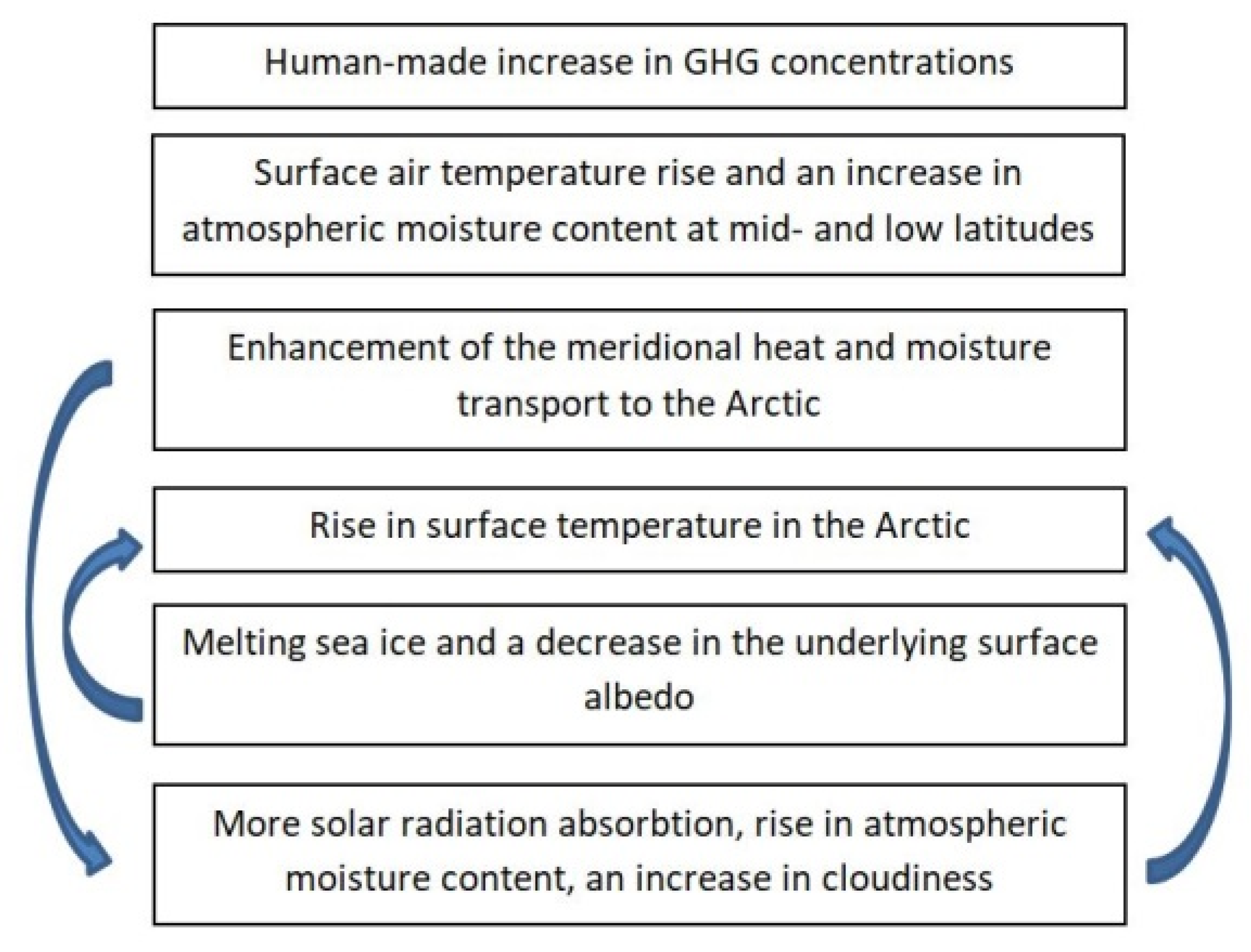
Despite the fact that the causal relationships in the climate system are quite complex and diverse and, moreover, not always clearly understandable, we can nevertheless suggest a very simplified qualitative picture of the Arctic climate formation resulting from meridional heat and moisture transport, and radiative feedbacks in the climate system (see Figure 6).

Figure 6.
A simplified diagram of the Arctic climate formation.
Unfortunately, the quantitative contribution of the meridional transport and feedback mechanisms to the formation of the Arctic climate is not yet entirely clear, and it has to be assessed both from observational data and from the results of experiments with climate models. In this paper, to assess the response of atmospheric meridional transport of sensible and latent heat to global climate change, we used a classic plane model of baroclinic instability. Within this theoretical framework, we obtained that an increase in GMST by results in an increase in atmospheric poleward heat and moisture transport by about 9% compared with the basic climate state. Undoubtedly, the plane model is an idealized atmospheric model, which is capable of describing only the development of baroclinic instability and the onset of synoptic-scale eddies at their initial stage. The full life cycle of eddies can only be described using three-dimensional mathematical models with parameterized physics. One of these models can be found in [75], where we explored the lifecycle of Arctic cyclone generation and evolution using a 3D mesoscale model of the atmosphere.
As shown in a number of previously published papers (e.g., [18,76,77]), complex climate models predict an increase in atmospheric equator-to-pole energy transport with climate change; however, this increase has large inter-model differences. Thus, a direct quantitative comparison of our results with the results of numerical climate model simulations is very problematic. It is important that the plane model allows for exploration of the meridional heat transport under different climate change scenarios. For this purpose, we need only to determine the static stability parameter and the vertical wind shear that correspond to a particular climate change scenario.
As suggested in [51], the greatest contribution to the warming of the Arctic climate is made by poleward heat advection (equator-to-pole heat transport). Therefore, we can reasonably expect that the state of the Arctic ice is also strongly influenced by the meridional heat transport, which changes due to global warming.
One further point must be taken into account with regard to feedback mechanisms. Since the strength of feedbacks is seasonally dependent [72], the poleward heat transport affects the Arctic climate differently in summer and winter periods. As shown in [48], the influence of feedbacks on the formation of the Arctic climate is much stronger in winter than in summer.
Meanwhile, it is necessary to emphasize that the results obtained in this paper should be approached with caution due to the simplicity of the applied model. The impact of global climate change on the Arctic climate formation and the Arctic sea ice extent can, without a doubt, be estimated using coupled climate models, which require enormous computational resources. However, simplified models such as those used in this study are very useful for better understanding the physical foundations of the dynamics of climate affected by external forcing.
Funding
This research received no external funding.
Institutional Review Board Statement
Not applicable.
Informed Consent Statement
Not applicable.
Conflicts of Interest
The author declares no conflict of interest.
References
- The Millennium Project. Global Futures Studies and Research. Available online: www.millennium-project.org/15-global-challenges (accessed on 24 December 2020).
- Bradley, R. Paleoclimatology: Reconstructing Climates of the Quaternary; Elsevier: Oxford, UK, 2015; 696p. [Google Scholar]
- NOAA National Centers for Environmental Information, State of the Climate. Global Climate Report. December 2018. Available online: www.ncdc.noaa.gov/sotc/global/201812 (accessed on 21 December 2020).
- IPCC 2013. Contribution of working group I to the Fifth assessment report of the intergovernmental panel on climate change. In Climate Change 2013: The Physical Science Basis; Stocker, T.F., Qin, D., Plattner, G.-K., Tignor, M., Allen, S.K., Boschung, J., Nauels, A., Xia, Y., Bex, V., Midgley, P.M., Eds.; Cambridge University Press: Cambridge, UK; New York, NY, USA, 2013; 1535p. [Google Scholar]
- NOAA Earth System Research Laboratory. Global Monthly Mean CO2. Available online: www.esrl.noaa.gov/gmd/ccgg/trends/global.html (accessed on 21 December 2020).
- Ripple, W.J.; Wolf, C.; Newsome, T.M.; Barnard, P.; Moomaw, W.R. World scientists’ warning of a climate emergency. BioScience 2019, 70, 8–12. [Google Scholar] [CrossRef]
- Santer, B.D.; Bonfis, C.J.W.; Fu, Q.; Fyfe, J.C.; Hegerl, G.C.; Mears, C.; Painter, J.F.; Po-Chedley, S.; Wentz, F.J.; Zelinka, M.D.; et al. Celebrating the anniversary of three key events in climate change science. Nat. Clim. Chang. 2019, 9, 180–182. [Google Scholar] [CrossRef] [Green Version]
- World Meteorological Organization. Inter-commission coordination group on WIGOS. In Proceedings of the Task Team on WIGOS Metadata (TT-WMD), Zurich, Switzerland, 27–29 November 2017; Available online: https://www.wmo.int/pages/prog/www/WIGOS-WIS/meetings/TT-WMD-6/TT-WMD-6_DocumentationPlan.html (accessed on 22 December 2020).
- AMAP. Snow, Water, Ice and Permafrost in the Arctic (SWIPA) 2017; Arctic Monitoring and Assessment Programme (AMAP): Oslo, Norway, 2017; 269p. [Google Scholar]
- Box, J.E.; Colgan, W.T.; Christensen, T.R.; Schmidt, N.M.; Lund, M.; Parmentier, F.-J.W.; Brown, R.; Bhatt, U.S.; Euskirchen, E.S.; Romanovsky, V.E.; et al. Key indicators of Arctic climate change: 1971–2017. Environ. Res. Lett. 2019, 14, 045010. [Google Scholar] [CrossRef]
- Bader, J.; Mesquita, M.D.S.; Hodges, K.I.; Keenlyside, N.; Østerhus, S.; Miles, M. A review on Northern Hemisphere sea-ice, storminess and the North Atlantic Oscillation: Observations and projected changes. Atmos. Res. 2011, 101, 809–834. [Google Scholar] [CrossRef]
- Stroeve, J.C.; Kattsov, V.; Barrett, A.; Serreze, M.; Pavlova, T.; Holland, M.; Meier, W.N. Trends in Arctic sea ice extent from CMIP5, CMIP3, and observations. Geophys. Res. Lett. 2012, 39, L16502. [Google Scholar] [CrossRef] [Green Version]
- Olonscheck, D.; Mauritsen, T.; Notz, D. Arctic sea-ice variability is primarily driven by atmospheric temperature fluctuations. Nat. Geosci. 2012, 12, 430–434. [Google Scholar] [CrossRef]
- Döscher, R.; Vihma, T.; Maksimoich, E. Recent advances in understanding the Arctic climate system state and change from a sea ice perspective: A review. Atmos. Chem. Phys. 2014, 14, 13571–13600. [Google Scholar] [CrossRef] [Green Version]
- Serreze, M.C.; Stroeve, J. Arctic sea ice trends, variability and implications for seasonal ice forecasting. Philos. Trans. R. Soc. A 2015, 373, 20140159. [Google Scholar] [CrossRef] [Green Version]
- Cvijanovic, I.; Caldeira, K. Atmospheric impacts of sea ice decline in CO2 induced global warming. Clim. Dyn. 2015, 44, 1173–1186. [Google Scholar] [CrossRef] [Green Version]
- Alekseev, G.V.; Glok, N.I.; Smirnov, A.V. On assessment of the relationship between changes of sea ice extent and climate in the Arctic. Int. J. Climatol. 2016, 36, 3407–3412. [Google Scholar] [CrossRef]
- Alekseev, G.V.; Glok, N.I.; Vyazilova, A.E.; Kharlanenkova, N.E. Climate change in the Arctic: Causes and mechanisms. IOP Conf. Ser. Earth Environ. Sci. 2020, 606, 012002. [Google Scholar] [CrossRef]
- Meredith, M.M.; Sommerkorn, S.; Cassotta, C.; Derksen, A.; Ekaykin, A.; Hollowed, G.; Kofinas, A.; Mackintosh, J.; Melbourne-Thomas, M.M.C.; Muelbert, G.; et al. Polar regions. In IPCC Special Report on the Ocean and Cryosphere in a Changing Climate; Pörtner, H.-O., Roberts, D.C., Masson-Delmotte, V., Zhai, P., Tignor, M., Poloczanska, E., Mintenbeck, K., Alegría, A., Nicolai, M., Okem, A., et al., Eds.; IPCC: Geneve, Switzerland, 2021; Available online: https://www.ipcc.ch/srocc/chapter/chapter-3-2 (accessed on 17 March 2021).
- Holland, M.M.; Bitz, C.M. Polar amplification of climate change in coupled models. Clim. Dyn. 2003, 21, 221–232. [Google Scholar] [CrossRef]
- Alexeev, V.A.; Langen, P.L.; Bates, J.R. Polar amplification of surface warming on an aquaplanet in “ghost forcing” experiments without sea ice feedbacks. Clim. Dyn. 2005, 24, 655–666. [Google Scholar] [CrossRef]
- Bekryaev, R.V.; Polyakov, I.V.; Alexeev, V.A. Role of polar amplification in long-term surface air temperature variations and modern Arctic warming. J. Clim. 2010, 23, 3888–3906. [Google Scholar] [CrossRef]
- Larsen, J.N.; Anisimov, O.A.; Constable, A.; Hollowed, A.B.; Maynard, N.; Prestrud, P.; Prowse, T.D.; Stone, J.M.R. Polar regions. Part B: Regional aspects. Contribution of working group II to the Fifth assessment report of the intergovernmental panel on climate change. In Climate Change 2014: Impacts, Adaptation, and Vulnerability; Barros, V.R., Field, C.B., Dokken, D.J., Mastrandrea, M.D., Mach, K.J., Bilir, T.E., Chatterjee, M., Ebi, K.L., Estrada, Y.O., Genova, R.C., et al., Eds.; Cambridge University Press: Cambridge, UK; New York, NY, USA, 2014; pp. 1567–1612. [Google Scholar]
- Lee, S. A theory for polar amplification from a general circulation perspective. Asia-Pac. J. Atmos. Sci. 2014, 50, 31–43. [Google Scholar] [CrossRef]
- Alekseev, G.V. Development and amplification of global warming in the Arctic. Fundam. Appl. Climatol. 2015, 1, 11–26. [Google Scholar]
- Previdi, M.; Janoski, T.P.; Chiodo, G.; Smith, K.L.; Polvani, L.M. Arctic amplification: A rapid response to radiative forcing. Geophys. Res. Lett. 2020, 47, e2020GL089933. [Google Scholar] [CrossRef]
- Hall, R.J.; Hanna, E.; Chen, L. Winter arctic amplification at the synoptic timescale, 1979–2018, its regional variation and response to tropical and extratropical variability. Clim. Dyn. 2021, 56, 457–473. [Google Scholar] [CrossRef]
- Serreze, M.C.; Barry, R.G. Processes and impacts of Arctic amplification: A research synthesis. Glob. Planet. Chang. 2011, 77, 85–96. [Google Scholar] [CrossRef]
- Laîné, A.; Yoshimori, M.; Abe-Ouchi, A. Surface Arctic amplification factors in CMIP5 models: Land and oceanic surfaces and seasonality. J. Clim. 2016, 29, 3297–3316. [Google Scholar] [CrossRef]
- Goosse, H.; Kay, J.E.; Armour, K.C.; Bodas-Salcedo, A.; Chepfer, H.; Docquier, D.; Jonko, A.; Kushner, P.J.; Lecomte, O.; Massonnet, F.; et al. Quantifying climate feedbacks in polar regions. Nat. Commun. 2018, 9, 1919. [Google Scholar] [CrossRef] [PubMed]
- Heinze, C.; Eyring, V.; Friedlingstein, P.; Jones, C.; Balkanski, Y.; Collins, W.; Fichefet, T.; Gao, S.; Hall, A.; Ivanova, D.; et al. ESD reviews: Climate feedbacks in the Earth system and prospects for their evaluation. Earth Syst. Dyn. 2019, 10, 379–452. [Google Scholar] [CrossRef] [Green Version]
- Notz, D.; SIMIP Community. Arctic sea ice in CMIP6. Geophys. Res. Lett. 2020, 47, e2019GL086749. [Google Scholar] [CrossRef]
- Matveev, L.T. Fundamentals of General Meteorology: Physics of the Atmosphere; Israel Program for Scientific Translation: Jerusalem, Israel, 1967; 720p. [Google Scholar]
- Hartmann, D.L. Global Physical Climatology; Academic Press: New York, NY, USA, 1994; 408p. [Google Scholar]
- Budyko, M.I. Climate and Life; Academic Press: London, UK, 1974; 507p. [Google Scholar]
- Monin, A.S. An Introduction of the Theory of Climate; Springer: Dordrecht, The Netherlands, 1986; 261p. [Google Scholar]
- Serreze, M.C.; Barry, R.G. The Arctic Climate System, 2nd ed.; Cambridge University Press: Cambridge, UK, 2014; 415p. [Google Scholar]
- Peixoto, J.P.; Oort, A.H. Physics of Climate; American Institute of Physics: New York, NY, USA, 1992; 520p. [Google Scholar]
- Mayer, M.; Tietsche, S.; Haimberger, L.; Tsubouchi, T.; Mayer, J.; Zuo, H. An improved estimate of the coupled energy budget. J. Clim. 2019, 32, 7915–7934. [Google Scholar] [CrossRef]
- Budyko, M.I. The effect of solar radiation variations on the climate of the Earth. Tellus 1969, 21, 611–619. [Google Scholar] [CrossRef] [Green Version]
- Sellers, W.D. A global climatic model based on energy balance of the Earth-atmosphere system. J. Appl. Meteorol. 1969, 8, 392–400. [Google Scholar] [CrossRef]
- Serreze, M.C.; Barrett, A.P.; Slater, A.G.; Steele, M.; Zhang, J.; Trenberth, K.E. The large-scale energy budget of the arctic. J. Geophys. Res. 2007, 112, D11122. [Google Scholar] [CrossRef] [Green Version]
- Oort, A.H.; Peixoto, J.P. The annual cycle of the energetics of the atmosphere on a planetary scale. J. Geophys. Res. 1974, 79, 2705–2719. [Google Scholar] [CrossRef]
- Nakamura, N.; Oort, A.H. Atmospheric heat budgets of the polar regions. J. Geophys. Res. 1988, 93, 9510–9524. [Google Scholar] [CrossRef]
- Porter, D.F.; Cassano, J.J.; Serreze, M.C.; Kindig, D.N. New estimates of the large-scale arctic atmospheric energy budget. J. Geophys. Res. 2010, 115, D08108. [Google Scholar] [CrossRef] [Green Version]
- Mayer, M.; Haimberger, L. Poleward atmospheric energy transports and their variability as evaluated from ECMWF reanalysis data. J. Clim. 2012, 25, 734–752. [Google Scholar] [CrossRef]
- Bengtsson, L.; Hodges, K.; Koumoutsaris, S.; Zahn, M.; Berrisford, P. The changing energy balance of the polar regions in a warmer climate. J. Clim. 2012, 26, 3112–3129. [Google Scholar] [CrossRef]
- Alekseev, G.V.; Kuzmina, S.I.; Urazgildeeva, A.V.; Bobylev, L.P. Impact of atmospheric heat and moisture transport on Arctic warming in winter. Fundam. Appl. Climatol. 2016, 1, 43–63. [Google Scholar] [CrossRef]
- Armour, K.C.; Siler, N.; Donohoe, A.; Roe, G.H. Meridional atmospheric heat transport constrained by energetics and mediated by large-scale diffusion. J. Clim. 2019, 32, 3655–3680. [Google Scholar] [CrossRef]
- Sorteberg, A.; Walsh, J. Seasonal cyclone variability at 70° N and its impact on moisture transport into the Arctic. Tellus 2008, 60A, 570–586. [Google Scholar] [CrossRef]
- Alekseev, G.V. Arctic dimension of global warming. J. ICE Snow 2014, 54, 53–68. [Google Scholar] [CrossRef]
- Alekseev, G.V.; Kuzmina, S.I.; Glok, N.I.; Vyazilova, A.E.; Ivanov, N.E.; Smirnov, A.V. Influence of Atlantic on the warming and reduction of sea ice in the Arctic. J. ICE Snow 2017, 57, 381–390. [Google Scholar] [CrossRef] [Green Version]
- Dee, D.P.; Uppala, S.M.; Simmons, A.J.; Berrisford, P.; Poli, P.; Kobayashi, S.; Andrae, U.; Balmaseda, M.A.; Balsamo, G.; Bauer, P.; et al. The ERA-Interim reanalysis: Configuration and performance of the data assimilation system. Q. J. R. Meteorol. Soc. 2011, 137, 553–597. [Google Scholar] [CrossRef]
- Held, I.M.; Hoskins, B.J. Large-scale eddies and the general circulation of the atmosphere. Adv. Geophys. 1985, 28, 3–31. [Google Scholar]
- Grotjahn, R. Baroclinic Instability. In Encyclopedia of Atmospheric Sciences; Holton, J.R., Curry, J.A., Pyle, J.A., Eds.; Academic Press: Cambridge, MA, USA, 2003; pp. 419–467. [Google Scholar]
- Lorenz, E.N. Available potential energy and the maintenance of the general circulation. Tellus 1955, 7, 157–167. [Google Scholar] [CrossRef] [Green Version]
- Soldatenko, S. Influence of atmospheric static stability and meridional temperature gradient on the growth in amplitude of synoptic-scale unstable waves. Atmos. Ocean. Phys. 2014, 50, 554–561. [Google Scholar] [CrossRef]
- Pfahl, S.; O’Gorman, P.A.; Singh, M.S. Extratropical cyclones in idealized simulations of changed climates. J. Clim. 2015, 28, 9373–9392. [Google Scholar] [CrossRef] [Green Version]
- Frierson, D.M.W. Robust increases in midlatitude static stability in simulations of global warming. Geophys. Res. Lett. 2006, 33, L24816. [Google Scholar] [CrossRef] [Green Version]
- Karamperidou, C. Surface temperature gradients as diagnostic indicators of midlatitude circulation dynamics. J. Clim. 2012, 25, 4154–4171. [Google Scholar] [CrossRef] [Green Version]
- Harvey, B.; Shaffrey, L.; Woollings, T. Equator-to-pole temperature differences and the extra-tropical storm track responses of the CMIP5 models. Clim. Dyn. 2014, 43, 1171–1182. [Google Scholar] [CrossRef] [Green Version]
- Soldatenko, S. Estimated impacts of climate change on eddy meridional moisture transport in the atmosphere. Appl. Sci. 2019, 9, 4992. [Google Scholar] [CrossRef] [Green Version]
- Holton, J.R. An Introduction to Dynamic Meteorology, 4th ed.; Academic Press: New York, NY, USA, 2004; 552p. [Google Scholar]
- Soldatenko, S.; Tingwell, C. The sensitivity of characteristics of large scale baroclinic unstable waves in southern hemisphere to the underlying climate. Adv. Meteorol. 2013, 981271, 10. [Google Scholar] [CrossRef]
- Blackmon, M.L.; White, G.H. Zonal wavenumber characteristics of Northern Hemisphere transient eddies. J. Atmos. Sci. 1982, 39, 1985–1998. [Google Scholar] [CrossRef] [Green Version]
- Akperov, M.G.; Mokhov, I.I. Estimates of the sensitivity of cyclonic activity in the troposphere of extratropical latitudes to changes in the temperature regime. Atmos. Ocean. Phys. 2013, 49, 129–136. [Google Scholar] [CrossRef]
- Hernandez-Deckers, D.; Von Storch, J.-S. Impact of the warming patterns on global energetics. J. Clim. 2012, 25, 5223–5240. [Google Scholar] [CrossRef]
- Soldatenko, S.A.; Chichkine, D. Climate model sensitivity with respect to parameters and external forcing. In Topics in Climate Modeling; Hromadka, T., Rao, P., Eds.; Intech Publishing: Rijeka, Croatia, 2016; pp. 105–135. [Google Scholar]
- Colman, R.; Soldatenko, S. Understanding the links between climate feedbacks, variability and change using a two-layer energy balance model. Clim. Dyn. 2020, 54, 3441–3459. [Google Scholar] [CrossRef]
- Roe, G. Feedbacks, Timescales and Seeing Red. Annu. Rev. Earth Planet. Sci. 2009, 37, 93–115. [Google Scholar] [CrossRef] [Green Version]
- Boeke, R.C.; Taylor, P.C.; Sejas, S.A. On the nature of the Arctic’s positive lapse-rate feedback. Geophys. Res. Lett. 2021, 48, e2020GL091109. [Google Scholar] [CrossRef]
- Block, K.; Schneider, F.A.; Mülmenstädt, J.; Salzmann, M.; Quaas, J. Climate models disagree on the sign of total radiative feedback in the Arctic. Tellus A Dyn. Meteorol. Ocean. 2020, 72, 1–14. [Google Scholar] [CrossRef] [Green Version]
- Årthur, M.; Eldevik, T.; Smedsrud, L.H. The role of Atlantic heat transport in future Arctic winter sea ice loss. J. Clim. 2019, 32, 3327–3341. [Google Scholar] [CrossRef]
- Docquier, D.; Fuentes-Franco, R.; Wyser, K.; Koenigk, T. Interactions between ocean heat transport and Arctic sea ice. In Proceedings of the EGU General Assembly, Online, 4–8 May 2020; Available online: https://meetingorganizer.copernicus.org/EGU2020/EGU2020-3352.html (accessed on 17 March 2021). [CrossRef]
- Soldatenko, S.A.; Matveev, L.T. On the effect of baroclinicity on the large-scale vortex formation in the atmosphere. Proc. USSR Acad. Sci. 1989, 308, 1103–1107. [Google Scholar]
- Hwang, Y.-T.; Frierson, D.M.W. Increasing atmospheric poleward energy transport with global warming. Geophys. Res. Lett. 2010, 37, L24807. [Google Scholar] [CrossRef]
- Liang, M.; Czaja, A.; Graversen, R.; Tailleux, R. Poleward energy transport: Is the standard definition physically relevant at all time scales? Clim. Dyn. 2018, 50, 1785–1797. [Google Scholar] [CrossRef] [Green Version]

Publisher’s Note: MDPI stays neutral with regard to jurisdictional claims in published maps and institutional affiliations. |
© 2021 by the author. Licensee MDPI, Basel, Switzerland. This article is an open access article distributed under the terms and conditions of the Creative Commons Attribution (CC BY) license (https://creativecommons.org/licenses/by/4.0/).