Abstract
Guaranteeing safety of navigation within the Netherlands Continental Shelf (NCS), while efficiently using its ocean mapping resources, is a key task of Netherlands Hydrographic Service (NLHS) and Rijkswaterstaat (RWS). Resurvey frequencies depend on seafloor dynamics and the aim of this research is to model the seafloor dynamics to predict changes in seafloor depth that would require resurveying. Characterisation of the seafloor dynamics is based on available time series of bathymetry data obtained from the acoustic remote sensing method of both single-beam echosounding (SBES) and multibeam echosounding (MBES). This time series is used to define a library of mathematical models describing the seafloor dynamics in relation to spatial and temporal changes in depth. An adaptive, functional model selection procedure is developed using a nodal analysis (0D) approach, based on statistical hypothesis testing using a combination of the Overall Model Test (OMT) statistic and Generalised Likelihood Ratio Test (GLRT). This approach ensures that each model has an equal chance of being selected, when more than one hypothesis is plausible for areas that exhibit varying seafloor dynamics. This ensures a more flexible and rigorous decision on the choice of the nominal model assumption. The addition of piecewise linear models to the library offers another characterisation of the trends in the nodal time series. This has led to an optimised model selection procedure and parameterisation of each nodal time series, which is used for the spatial and temporal predictions of the changes in the depths and associated uncertainties. The model selection results show that the models can detect the changes in the seafloor depths with spatial consistency and similarity, particularly in the shoaling areas where tidal sandwaves are present. The predicted changes in depths and uncertainties are translated into a probability risk-alert map by evaluating the probabilities of an indicator variable exceeding a certain decision threshold. This research can further support the decision-making process when optimising resurvey frequencies.
1. Introduction
The bathymetric surveying necessary for accurate nautical charts and adequate maintenance dredging is a joint responsibility of the Netherlands Hydrographic Service (NLHS) and Rijkswaterstaat (RWS). The seabed mapping is conducted using the active, acoustic remote sensing method of single-beam echosounding (SBES) and multibeam echosounding (MBES). This continuous mapping is a national responsibility and adheres to the SOLAS (Safety of Life at Sea) V convention developed by the International Maritime Organisation (IMO) and is also in accordance with the International Hydrographic Organisation (IHO), Special Publication No. 44 (S44) hydrographic survey standards. The Netherlands has developed and refined its own survey policy, designed to complement the set of standards provided by the IHO S44 standards [1,2].
The Dutch economy is heavily reliant on the activity in the Ports of Rotterdam and Amsterdam and safe navigation in the waterways to these ports, particularly for deeper draught vessels, is considered crucial to prevent risk to vessel grounding. The fundamental knowledge of seabed dynamics in relation to the changes in depths is therefore an important factor to consider for safety of navigation, maintenance of channels and hence for optimising the resurvey policy where the overall aim is to provide timely and accurate predictions of the changes in seafloor depths as a resurvey decision-making tool. This can also ensure more cost-effective and efficient use of the mapping resources given the extensive use of the NCS and the nature of the oceanographic and seafloor properties which make it a complex marine environment.
The NCS is characterised as being a shallow sea, average depth 40 m with a sandy seafloor (typical grain sizes of 0.4 mm, though the spatial distribution of the grain sizes differ) and results in regions of the NCS with varying seabed dynamics i.e., sandbanks which are aligned parallel to the current flow and sandwaves and smaller megaripples which are transverse to the flow [3,4]. Previous research [5,6,7,8], emphasised that characteristics of sandwave features are of the greatest concern in the North Sea since sandwaves vary in amplitudes up to tens of meters, wavelengths in the order 100–1000 m and have migration rates of up to 10 m per year. The migration of the sandwaves are caused by residual currents [4] and tidal asymmetry [9].
For optimisation of resurvey frequencies based on the available time series of bathymetry data, this paper considers an area where tidal sandwaves present challenges to safety of navigation. The library of functional models is characterised to estimate the main parameter of interest, changes in seafloor depth. This required defining the functional and stochastic models using the time series of available bathymetry data. The development of the methodology uses statistical hypothesis testing applied to a library of functional models, to arrive at the most likely model which can be used for predicting the changes in the depths with associated confidence intervals. This method of deformation analysis using time series was also previously studied in [7,10,11,12]. Studies by [7,12] analysed areas in the 0D (zero-dimensional, per grid node or a nodal analysis), 1D (one-dimensional, line analysis in the directions of maximum and minimum variability) and 2D (planar analysis). A 0D, nodal analysis was also conducted by [8]. These studies concluded that the disadvantage of the 1D and 2D analyses, both required an assumption of the sandwave dynamics in the area of study and hence limited to a fixed area definition.
For this paper, a 0D spatial analysis was chosen to determine the most likely functional model to avoid any spatial assumptions on the seafloor dynamics when defining the library of functional models. An advantage of the choice of 0D analysis is that the patterns related to temporal trends in the changes in depths can be revealed for different nodes (e.g., the crests and the troughs) whereby a distinction can be drawn since they may exhibit different behaviours. In deformation studies such as in [10,13] a 0D approach was also taken and in the case of ground deformation in [14] using Interferometric Synthetic Aperture Radar (InSAR) point scatterers, adding flexibility to the applicability of the 0D approach.
The choice of parameterisation of the spatial and temporal dynamics is achieved by defining a minimal set of model parameters to describe and predict the changes in the depths and associated uncertainties. This primary problem required defining a library of simple, functional models to determine whether changes in depths can be detected by testing mutually exclusive alternatives. Due to the morphological characteristics and migration of sandwaves and hence the time of increase or decrease in the depth within a time series, the parametric models aim to estimate the changes in shallowest likely depth (for the case of safety of navigation which is depicted on nautical charts).
The method is developed to automatically select from the library the most likely model for a reliable prediction. To find a functional model that accurately describes the characteristics of the changing seafloor, it was necessary to take into account the variability of the observations with an a priori stochastic model based on the measurements and gridding process. This functional model selection procedure has been developed based on statistical hypothesis testing and can be viewed as an adapted version of the Detection, Identification and Adaptation (DIA) procedure from [15,16].
Additionally, the functional models selected and the prediction of the changes in depth are used to develop an approach for a risk-alert system for different applications such as safety of navigation, exposure of pipelines and cables on the seafloor [4] and the regeneration of sandwaves after human intervention such as maintenance dredging [17]. This is done by translating the predicted uncertainties of the changes in the depths to estimated probabilities and further evaluating when depth change exceeds a decision threshold. The choice of threshold levels serves as the basis for determining risk-alert levels using quality indicators as a tool for decision-making when improving the planning of resurvey frequencies in the NCS.
For this research, the time series was limited to the preprocessed bathymetry data acquired from SBES and MBES since this combination provides the most accurate measurements, increased coverage and high resolution with regards to MBES, for detecting changes in the depths for the aforementioned applications. This research provides added value to use the methodology developed to assimilate and synthesise depth observations and associated uncertainties derived from other remote sensing techniques such as bathymetric LIDAR (light, detection and ranging) [18], bathymetry retrieval from synthetic aperture radar (SAR) [19] and satellite derived bathymetry (SDB) [20,21,22]. For the NCS however, the efficient use of optical remote sensing techniques such as bathymetric LIDAR and SDB are limited due to reduced water clarity and low turbidity requirements for monitoring bathymetric changes for applications with high accuracy requirements as opposed to MBES.
Although the primary research application for this paper is safety of navigation for optimising resurvey frequencies, other related scientific research in the fields of coastal sea level rise, coastal geomorphology, marine conservation, ocean circulation modelling and marine infrastructure development all rely on the most recent bathymetry data as the basis for their research where monitoring of seafloor changes is essential.
Figure 1 shows the present categorized subdivision of the NCS and the corresponding survey frequencies (’Opnameplan’) which vary from critical areas, once every 2 years to other areas, once every 4 years, 10 years, 15 years and 25 years, as published within the NLHS organisation in 2017. Due to varying circumstances, the NLHS have not achieved some of these survey frequencies over recent years [7], which makes the prediction and hence the probabilistic risk-alert system using the available time series of bathymetry even more relevant to resurvey planning and decision-making.
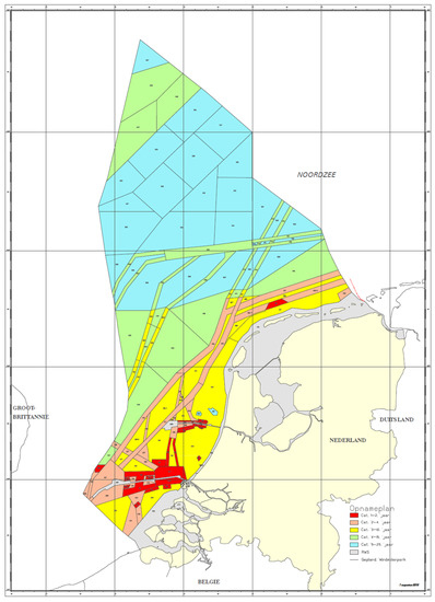
Figure 1.
Map of Netherlands Continental Shelf resurvey frequencies, courtesy of NLHS 2017. The Categories are listed from Cat 1 (red) to Cat 5 (cyan) with respective resurvey frequencies once every 2 years, 4 years, 10 years, 15 years and 25 years. The nearshore grey areas are the responsibility of RWS.
The main objectives of this research are (a) the definition of additional functional models which can be used to describe the complex behaviour of the changing seafloor depths especially where sandwave features are present (b) designing a more rigorous approach to select the nominal model to be used in the testing procedure and (c) designing the statistical hypothesis testing procedure to allow for reliable prediction and evaluation of probabilities for risk-alert levels.
The contribution of this research is arranged first with the detailed methodology in Section 2. This section outlines the library of functional models and the description of the stochastic model used for the hypothesis testing procedure developed. The prediction and validation step using the selected functional models is also described here. Section 3 presents the results and discussion of the methodology applied for a site-specific case study area that exhibits tidal sandwave features. Section 4 presents the results of the prediction and uncertainties using the selected models. Section 5 introduces the probability estimation that the indicator variable will exceed a decision threshold, leading to a probability risk map. Section 6 summarises the findings and contributions made.
2. Methodology
2.1. Preparation of Bathymetry Time Series
Remote sensing technology of SBES and MBES systems provided the time series of bathymetry measurements used for this research. The time series are preprocessed archived data retrieved from the digital Bathymetric Archive System (BAS) of the NLHS and RWS. NLHS is responsible for the mapping of deeper areas greater than 10 m isobath and RWS, the shallower waterways, nearshore coastal zones and the maintenance of approach channels to port areas [8].
The quality of the archived data is assumed to be at least precise as the IHO S44 standards Order 1 at the 95% confidence level and have been preprocessed and cleaned to remove gross errors and to correct any systematic errors introduced [23]. The high resolution MBES datasets provide an observation at a minimum resolution of 3 m × 5 m. For SBES datasets, there is a minimum line spacing of 50 m and can increase up to 125 m and for this reason interpolation of the SBES surveys for gridded digital elevation model (DEM) generation is necessary. The available time series of bathymetry is in the geodetic datum WGS84 in the UTM Zone 31N projection and the depths are reduced to Lowest Astronomical Tide (LAT).
For the preparation of the time series, there are options for the original data to be gridded on a uniform grid (for e.g., 5 m × 5 m) or using a new quadtree approach [24] for creating a multi-resolution DEM, taking into account the heterogeneity of the data in space and time and the variability of the depths. This allows for optimal use of the time series of data available without loss of details in the final, resulting DEM [25]. Previous research [25] suggested the optimal criteria and standard deviation threshold (measure of variability within a grid cell), values for this application. These suggestions are still flexible depending on the end-users’ requirements. The quadtree approach also uses a time ordered approach to store the depths for each epoch or survey moment [25]. Figure 2 shows an example of a single epoch decomposition with m.
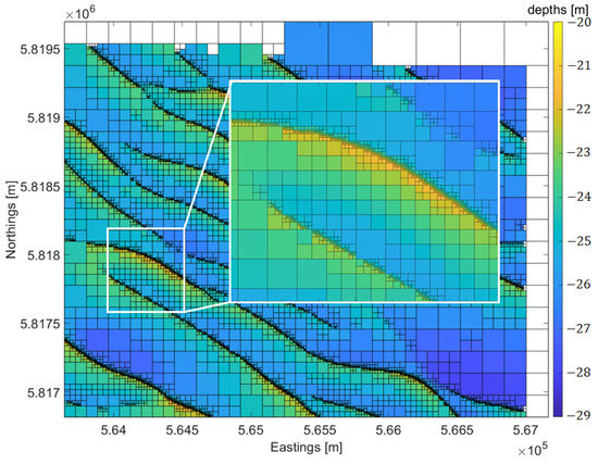
Figure 2.
Example of a single epoch quadtree decomposition for creating a multi-resolution DEM. Inset image shows a subset area of larger depth variability (sandwave features) where a minimum grid cell size of 5 m is obtained near the crest of the sandwaves.
The input data are therefore gridded so that each grid node represents the mean depth, its variance value and the time of survey defined by the year and month. The variance of each gridded depth value is a combination of the measurement uncertainty (provided by the standards [1]) and the spatial uncertainty (which takes into account the number of observations per grid cell). In [7] the size of the grid cells was limited to 50 m × 50 m and in [8] 25 m × 25 m. For SBES data that requires interpolation, the stochastic interpolation method of Universal Kriging [26] is applied which provides the gridded depth values d and the uncertainty, . Previous studies of [8,27] applied a vertical nodal analysis using linear regression for each node, excluding an uncertainty analysis of the estimated vertical trend as opposed to this contribution. The time series analysis requires the following input:
- Fixed grid node positions using quadtree DEM, .
- Time series of surveys, where n is the total number of epochs.
- Observed depths values, d for each grid node, p for each epoch.
- Variances of depths, per grid node , per epoch.
2.2. Specification of Stochastic Model
The quality of the input bathymetry is a source of uncertainty that can affect the quality and reliability of the DEM and hence the prediction. There are several sources of uncertainties in depth and position measurements since the system of measurement has a combination of its own uncertainties e.g., GPS, gyro and motion sensor. Additionally environmental factors such as sound speed profile, tides and draft. In addition, the uncertainty due to the spatial and interpolation errors needs to be taken into account.
2.2.1. Multibeam Echosounding Variances
The MBES datasets are considered full coverage with a minimum spatial resolution of 5 m × 3 m for each depth measurement, essentially requiring no interpolation. This suggests that the propagation of the MBES uncertainties are a combination of the measurement uncertainties which are derived from the IHO specifications Order 1 and the spatial variability from the gridding technique where the variance of the mean as the estimator is considered.
A main contribution to the DEM uncertainties is thus the measurement uncertainties. This is provided by the IHO standards which suggest the maximum allowable vertical and horizontal uncertainties for each depth measurement resulting from the data collection process [1]. The specifications suggest the maximum, vertical uncertainty for different survey orders depending on the survey priority (which is depth dependent for risk-alert management and safety of navigation) is computed using:
Here, a is the coefficient representing the uncertainty that does not vary with depth, b is the coefficient representing the uncertainty that is depth dependent and d is the reduced depth [1]. Sources of errors for the depth measurements and their variances can be used as in [7] where it includes the errors introduced by the echo sounder, sound velocity measurements, static draft measurement, dynamic draft, water level or tidal reduction, heave, pitch and roll. For MBES surveys, variances of the depths are assumed to be at least as precise as the IHO S44 standards of Order 1 uncertainty at the 95% level. Survey Order 1 specifies the depth precision for MBES data as in Equation (3) where the coefficients for computing in Equation (1) are m and respectively.
Other errors are the spatial variability of the depths within a specific grid cell size. The grid cell depth is calculated as a (weighted) average of observations in that cell, and uncertainties due to different interpolation or gridding techniques when the data are sparse [28,29]. The spatial uncertainty is therefore attributed to the grid cell size and the number of observations per grid cell. Hence, the grid cell uncertainty footprint can be estimated using:
where is the spatial uncertainty, is the standard deviation threshold and N, the number of observations within a grid cell. It is assumed that the underlying seafloor is flat or has a stationary mean. This is done during the quadtree decomposition phase as in [25] where the criteria for creating a multi-resolution grid are discussed. Three options are considered when storing the mean depth value for each quadtree grid cell. Spatial homogeneity is assumed when the number of observations is greater than 5 and the sample variance of the depth observations within each grid cell is less than the variance threshold value of m. The total vertical uncertainty of each stored, mean depth value is computed using Equation (2). This estimation is also applied to grid cells where there are less than 5 observations and the grid cell size is considered to be small (less than or equal to 10 m). If, however, there are instances where there are not enough observations within a grid cell, the search area is increased by doubling the current grid size and applying Equation (3).
2.2.2. Single-Beam Echosounding Variances
For SBES surveys performed between 1991 and 2003, the total propagated uncertainty in the depth measurement is also a function of various stochastic influences. These stochastic influences include the effect of sound speed velocity, heave, positioning and tidal reduction [7,23] resulting in a posteriori estimate of the variances. For SBES measurements the variances are predominantly due to the interpolation errors, since SBES techniques do not provide full coverage mapping of an area. The geostatistical method of Universal Kriging [30] is used which was adopted from [7] and the DIGIPOL algorithm in [31]. This method models the spatial variability of the seafloor using a Gaussian covariance function. The expected similarity of the observations and the interpolated positions are therefore modelled as a function of distance and direction [23]. The universal kriging provides both the gridded depths and their variances. The total propagated variance for SBES surveys is computed using:
as in [7].
2.3. Estimated Parameters
The method of Best Linear Unbiased Estimation (BLUE) was used for the estimation of seafloor parameters of the areas selected and the associated uncertainties. Previous studies made assumptions to allow for one-dimensional analyses (1D). The 1D analysis approach required a fixed definition of the areas that are considered uniform in sandwave dynamics and that the depths be gridded using a regular gridded structure. This was a requirement for the 1D analysis used in [7,12] to allow for the characterisation and detection of sandwave dynamics per grid line, in the direction of maximum spatial variability.
For the 0D analysis of an area, there are no a priori assumptions about the areas being homogeneous or exhibiting uniform morphodynamics. Because of this, the size of the areas to be analysed is only limited due to computational time (typically 25–30 min per 3 km × 3 km sub-area). Nodal parameter estimation of seafloor dynamics was studied by [10] and point wise estimation of other deformation parameters applied to geophysical processes and infrastructure using InSAR was studied by [14]. This choice of analysis is based on the available time series data and how we choose to parameterise the changes in depths. This parameterisation is a crucial step that is reliant on the changes that are important in relation to the applications. The advantages of this approach in comparison to the 1D and 2D approaches is that the vertical nodal dynamics will be able to capture the temporal changes in the depth.
The application of deformation analysis for predicting the changes in seafloor depths uses mathematical models as the expression of the relationship between the depths at the gridded locations to the unknown parameters of the model that describe the seafloor. The mathematical model is therefore a combination of the functional and stochastic model:
Here is the m-vector of depth observables, x is the n-vector of unknowns, A is the design matrix describing the assumed linear relation between and x, is the variance matrix, the m-vector of random measurement errors. and are the expectation and dispersion operators, respectively.
Since it is common to assume the observations are normally distributed, the estimators or library of functional models, with being a linear function of x is also a general linear Gauss-Markov Model for computing the BLUE of :
The principle of BLUE implies that the estimator must ensure minimum variance and must be unbiased. The BLUE [32] of the unknown parameters , the adjusted observations and the residuals are obtained by:
The precision of the estimator is given by:
from which can be seen that it depends on the precision of the observations , the design matrix A and therefore also on the redundancy or the degrees of freedom (DOF) . The estimated residuals in relation to the variance matrix affect the decision on the choice of the most likely model and the estimated parameters used for the seafloor estimation.
2.4. Functional Model Selection
To characterise the spatial and temporal change of the depths, this behaviour is modelled as a function of the available observations per epoch, t, per grid node. To determine the most appropriate characterisation and hence the model to be used to best describe and predict the behaviour, we apply statistical hypothesis testing in linear models [15]. Prior to applying the hypothesis testing procedure developed, a w-test is performed as a check, for any large errors within the observational data sets, i.e., any outlying survey within the time series [16].
This procedure then starts with a general, goodness of fit approach by defining a library of functional models or multiple hypotheses where where m is the number of hypotheses per time series. This library selection was designed during the exploratory data analysis [33] of the time series of the depths per node (0D) to identify patterns. In addition, empirical studies on the formation and analysis of sandwaves such as [27,34,35] were reviewed. Additionally, the purpose of the predictions was defined i.e., for the purposes of risk-alert management since the extreme changes in the depths pose a concern for safety of navigation, stability of offshore structures and exposure of pipelines and cables on the seafloor.
The seafloor characterisation in time, consists of a library of models using four levels of complexity (refer to Figure 3). The number of hypotheses in the library can be expanded with newly defined characterisations depending on the purpose of each case study. In this instance, the characterisations are kept simple to avoid over-fitting and additional parameter estimations which do not add to the understanding of the behaviour of shoaling depths in NCS. Additionally, the current library considers physically realistic characterisations that can detect and identify significant changes in seafloor depths at any given epoch in the time series. To identify the changes in depth before and after dredging moments, i.e., human intervention, the piecewise linear model characterisation would also prove useful.
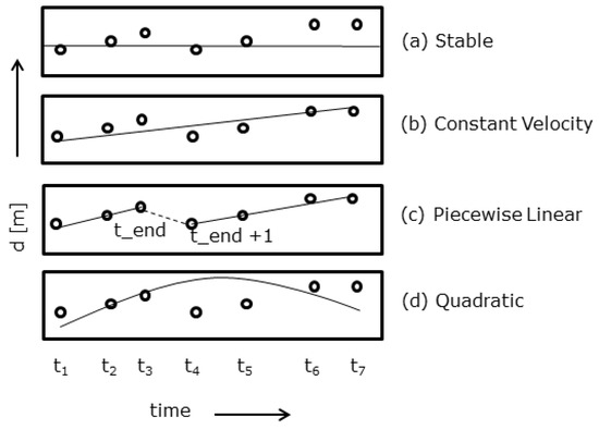
Figure 3.
Temporal seafloor characterisations (updated from [7]).
The simplest characterisation is represented by a horizontal line where is constant and is the only unknown parameter. The estimated constant depth is also the mean:
Another characterisation, adds the additional slope parameter, creating a constant velocity model with two unknown parameters, initial depth, and slope, :
The quadratic model has three unknown parameters where a is the acceleration and and are the estimated, initial depth and slope parameters respectively:
For the piecewise linear characterisation, the model consists of two separate line segments, i.e., for each node, depending on the length of the time series, several piecewise linear models are constructed with a breakpoint at each epoch with the restriction that there is a minimum of two observations at the start and end of each line segment creating the piecewise linear model, refer to Figure 3c. The piecewise linear characterisation consists of four unknown parameters, an initial depth and slope for each line segment respectively, , , and :
Here is the number of piecewise linear models, where , where m is the number of observations. Figure 3 shows the illustrated representation of the characterisations for each model equation.
The total number of hypotheses listed in Table 1, is expanded to include the varying number of piecewise models, per time series and therefore the total number of models is more than four per time series.

Table 1.
List of hypotheses for nodal analysis and unknown parameters.
Similar to previous research studies such as [7,14], this approach does not a priori assume that one hypothesis is more likely than the other, as is the common approach in classical hypothesis testing [15].
To describe the overall model inconsistency separately, for each of the functional models, the general expression of the Overall Model Test (OMT) statistic is first applied and defined as in Equation (13), where i represents the model number and j the node. The OMT statistic gives the quality of the model approximation by observing the relationship between the residuals, , which is the difference between the observations and the adjusted observations using the estimated parameters of the model and the uncertainty of gridded depth values defined by the diagonal of the variance-covariance matrix .
The OMT statistic is computed separately for all competing models and is compared to a critical value, . The OMT statistic follows a central chi-squared distribution with DOF as in Equation (14). This test statistic is computed by defining a critical value , where is the probability of falsely rejecting the OMT. This is also referred to as the probability of a false alarm or a Type I error, which should be low to unnecessarily reject a valid hypothesis and therefore the choice of , or level of significance, is usually chosen to be a small number [16] and can also vary depending on the goal of the analysis [7]. For this contribution the choice of is for step 1(a) as in Figure 4.
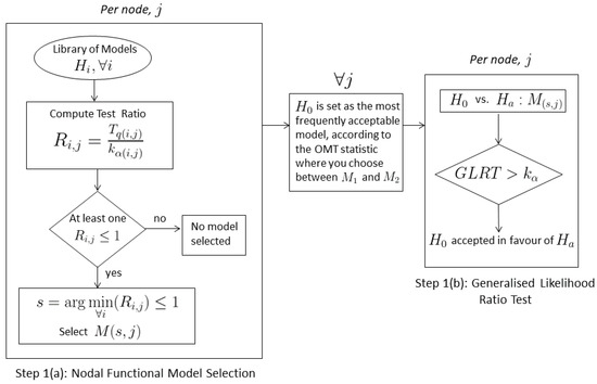
Figure 4.
Testing procedure for the functional model selection using time series per grid node.
Since the library of models vary in complexity and hence has different dimensions, these models will follow different distributions. This implies that when comparing the goodness of fit of these models, Equation (13) cannot be used. Instead, to account for the varying complexity of the models (more unknown parameters could result in over-fitting), the test statistic in Equation (13) can be normalised by dividing by the critical value, denoted by the statistical significance, . The test ratio value for each node is defined in Equation (15).
Based on Equation (15) there can be three outcomes for the nodal analysis:
- Only one model results in . Then, that model is selected for that particular node.
- More than one model can result in . Among the competing models, for each node j, findThen is selected for that node.
- If no model is accepted based on Equation (16), then none of the models is selected for that node.
The limitations of selecting the most likely model per node, , using these criteria only, are as follows:
- The values of two or more of the test ratios can be quite close to each other. Hence the associated models fit almost equally well.
- Due to irregularities in the data it can occur that the piecewise linear model is accepted, although in reality the constant velocity model should be selected. Additionally, the length of the time series and the larger number of unknown parameters in the piecewise linear model can result in over-fitting.
- The spatial correlation between the nodes is not accounted for and hence the selected models in the neighbouring nodes can show inconsistency, especially in areas of high variability.
To avoid misinterpretation, an area-wide assessment is done to make a decision on the choice of . This is done by selecting the most frequently, acceptable model, according to the OMT statistic, where the choice is between and as the default models for the initial assumption of general, area-wide dynamics. Between and , the model resulting in the maximum number of grid nodes is set as the model. This approach effectively makes the choice of more adaptable according to the sub-area of interest. This is different from current practice and previous research studies such as [7,14,36,37] where the OMT statistic is applied to a steady-state assumption of .
Where there are nodes for which the alternative model, is preferred instead of the null assumption, , this could imply that there are errors (disturbances or anomalies). This is another way of testing for large errors in the observations. We assume the m × 1 vector of observations is normally distributed with known variance matrix :
The following two hypotheses for two competing models are
and
For the alternative hypothesis, number of additional unknown parameters ∇ ( 0), with vector length q is introduced and is related to the expectation of by the m × q matrix [15]. The General Likelihood Ratio Test (GLRT) provides a decision on whether or not the additional variables in ∇ as in Equation (19) should be taken into account [15].
The GLRT in step 1(b) as in Equation (20) is then applied for each grid node separately using the two competing models where the null assumption and the alternative model, , is set as the assigned model, per grid node after step 1(a). is rejected in favour of if the GLRT value is greater than the critical value, :
The choice of for step 1(b) is and is moderately larger than the choice of for step 1(a) which was chosen as . This tradeoff is needed to minimize the effects of a missed detection and to thus maintain the probability of a correct decision after applying the GLRT in step1(b). This implies that if an alternative model, is preferred according to the level of significance and the degrees of freedom (DOF), then the detection of a deviation from will be correctly detected and hence will be rejected when is false. This is done by keeping the choice of for step1(b) small to ensure that is high. The power of test is defined as:
The least squares residuals for the null hypothesis, and the alternative hypotheses, are defined as:
2.5. Prediction and Validation Using Selected Functional Model
Once the final selected model, has been selected as the most likely model using the procedure outlined in Figure 4, this model can be used to describe the evolution of the depths in time, t. The present resurvey frequency map defines the next expected resurvey time, though in practice, it may not always be possible to resurvey according to the planned resurvey frequency. In [7], to predict the depths, the next epoch (in years) is denoted as as:
where the average period between surveys, was used as the predicted time and as the last available epoch.
For this research, the average period used is two years for the results presented in Section 3. is a flexible input parameter to ensure the use of short- and long-term prediction times, without the use of predetermined resurvey frequency times.
The predicted depths are represented as an M × 1 vector as:
is the known matrix and is the estimated unknown parameter vector representative of the selected model, . The precision of the predictions is obtained from the variance-covariance matrix by converting the main diagonal into a column of variances, , once the precision of the estimated parameters is also defined, as:
An example of this principle is given in Figure 5 where the 95% and 99% confidence interval around the estimated trend and the predicted trend have been constructed.
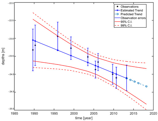
Figure 5.
Example showing the principle of the observed depth, d in relation to the estimated trend (BLUE) and predicted trend, including the 95% and 99% confidence interval around the estimated trend and the predicted trend.
To provide insight about the reliability and hence the predictive performance of the selected functional models, cross-validation is necessary. The leave-one-out cross-validation (LOOCV) approach [38,39] has limitations due to the short length of the time series and the modelled temporal trends between observations in the time series. To preserve this time ordered dependency during the functional model selection and to ensure a validation procedure, an approach is implemented whereby the time series is extended and hence DEMs and the associated uncertainties are created using simulated observations at the predicted times. To achieve this, the final selected model, was used to solve the forward model using the estimated parameters of . The error distribution, , for the simulated observations, , is defined as:
where is defined as the variance of the last observation in the time series. This is derived as the square root of the last element of the variance matrix . We assume that the simulated observations at different prediction times (refer to Equation (23)) can be obtained by simulating the random error which is added to the predicted observations as in Equation (24), based on the forward model and is given by:
With the simulated DEMs, several options can now be applied to assess the cross-validation error, for an area, i.e., the mean absolute errors for the total number of nodes per area J. First, for the prediction time , the average period used is two years, therefore, the absolute errors between the predictions , two years after the last survey moment and simulated observations are computed to obtain the as:
Figure 6 gives an example of the simulated observations, at the last survey moment and different predicted times, where (years) is [1 2 3 4 5 10 15 30] using the forward model or estimated trend (BLUE) and predicted trend, including the 95% confidence interval.
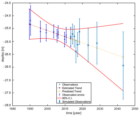
Figure 6.
Example showing the simulated observations at last survey moment and predicted times, where (years) is [1 2 3 4 5 10 15 30] using the forward model or estimated trend (BLUE) in relation to the observed depths, d and predicted trend, including the 95% confidence interval.
Additionally, since the time series can be extended using the simulated observations and the prediction time, is a flexible input parameter, another option can be applied whereby the simulated DEMs are used to further extend the length of the existing time series of the model selection procedure described in Figure 4. This model selection procedure can then be re-executed to evaluate the for an area and prediction time of interest.
3. Results of Spatial and Temporal Testing
In this section, the spatial and temporal results of the model selection procedure developed are presented for a sub-area within the IJgeul Approach area, West of IJmuiden. In the previous section the methodology for selecting the most likely functional models per grid node and the specification of the stochastic model were outlined. In Section 2, the functional models are different with respect to the specification of each design matrix, A and the stochastic models are the same throughout the testing procedure. The initial assumption of what is known about the general dynamics, that is the null model, , is selected based on the a priori assumption that each model is equally likely and follow the procedure step 1(a) in Figure 4 of Section 2. The resulting model after step 1(a) which is the most frequently accepted model, gives the corresponding null assumption of the general known dynamics of the area. This result proves to be a good assumption since the results of the model selection show spatial similarities after the GLRT between vs. is applied as in step 1(b).
3.1. Area West of IJmuiden
To test the method using real observations, the area IJgeul shown in Figure 7, located West of IJmuiden, is selected as the case study which was also analysed by [7] since it is an area exhibiting sandwave features. This area is subdivided into 30 sub-areas each of approximately 3 km × 3 km or less. Three sub-areas are the approach anchorage areas, namely AA, AB and AC. A list of the surveys available according to acquisition dates for the whole area is given in Table 2. For positioning, intentional degradation of the GPS signals are referred to as Selective Availability (SA). The older surveys (prior to 1996) used the terrestrial Hyperfix system, which provides the same order of uncertainty as the differential GPS (DGPS) with SA, i.e., in the order of 10 m. All surveys after 1996 used DGPS with SA [7]. According to the resurvey planning, the IJgeul area is resurveyed on average once every 2 years.
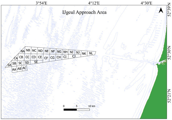
Figure 7.
Location of the IJgeul Approach area subdivided into 30 smaller sub-areas and 5 m bathymetry contour. Areas AA, AB and AC are the anchorage areas.
Table 2.
List of surveys, SBES and MBES (indicated by the line spacing) survey code and the start date. Datasets for each sub-area vary based on available overlapping survey data. Data and further information regarding access to data source can be found at https://publicwiki.deltares.nl/display/OET/Dataset+documentation+bathymetry+NLHO (accessed in June 2018).
Results for Sub-Area NF
Figure 8a shows the number of epochs per grid node, which is the length of the time series available per grid node for the sub-area NF. The majority of area NF has a time series length per grid node of 10 available epochs which spans 24 years from 1989 to 2013. The edges of this sub-area show a decrease in the length of the time series because of the size of the buffer areas used to subdivide the whole area into smaller sub-areas in a preprocessing step. However, of the sub-area has a length of time series of 10 which indicates a minimum DOF of 6. Figure 8b shows the computed test ratio, for the selected model in step 1(a). The spatial distribution of shows larger values on the crests of the sandwave features, where there is higher variability in the depths and hence larger residuals after model fitting. Although there are spatial consistencies different models are accepted in step 1(a), mostly to . Close to of the total number of nodes are selected for the stable model, and the constant velocity model during step 1(a).
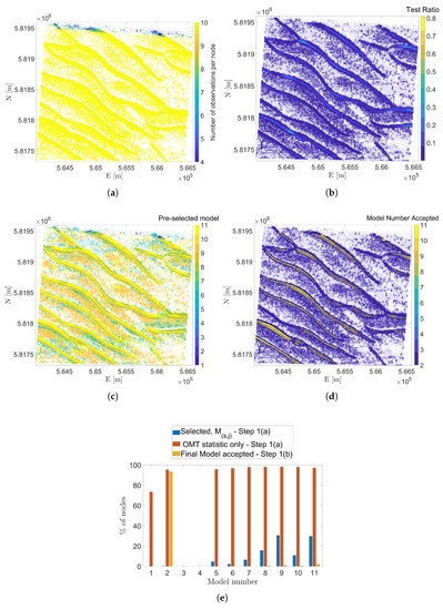
Figure 8.
Results after applying testing procedure outlined in Figure 4. Showing per node (a) Number of observations, (b) Test Ratio values, for selected models after step 1(a), (c) Selected Models, per sub-area after step 1(a), (d) Final accepted models after applying step1(b) and (e)% of nodes and corresponding models accepted under step 1(a) and step 1(b) resulting in , and the final selected models respectively. The most frequently acceptable models under the OMT statistic only is also shown.
Figure 8c shows how often a certain model was accepted after step 1(a). However, to avoid misinterpretation due to the limitations outlined in Section 2.4, it is also evaluated which models would be accepted based on the OMT for each node (’OMT statistic only’). From this, it follows that is the most realistic model to describe the general dynamics of the sub-area, and is therefore selected as the null hypothesis in step 1(b).
After setting the assumption to , the GLRT is performed between vs. . Figure 8d shows the models that are accepted after Equation (20) is applied where is accepted or rejected in favour of one of the alternative models. The resulting models accepted in Figure 8d show that of the nodes accepted and the remaining accepted one of the alternative piecewise models, to where of those remaining nodes accepted . Model numbers, are characterised as the piecewise linear function and the acceptance of these models is consistent along the crest of the sandwaves where there is higher variability in the depths due to the shape of the sandwave features.
The piecewise linear models are able to identify a significant change in depth, , where a stable, , constant velocity, or quadratic model, is not adequate to identify the changes between two constrained time intervals, and . This is further validated through visual inspection of the time series of the observations at selected nodes. Figure 9 shows a zoomed-in section of area NF and the time series of the nodes selected, numbered 1 to 6 in Figure 10.
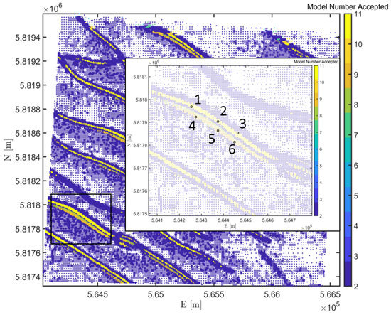
Figure 9.
Zoomed-in section of sub-area NF, showing nodes numbered 1–6 where an alternative model (piecewise linear model), is accepted in favour of (constant velocity model).
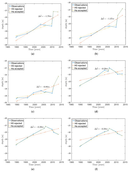
Figure 10.
Visual inspection of the time series of nodes, numbered 1 to 6, as in (a–f), showing the accepted models where is accepted in favour of .
By visually inspecting the plots in Figure 10, it shows that the accepted models are consistent with the observations in the time series which implies that the change was not misinterpreted as a flat or constantly sloping seafloor. Hence, the testing procedure correctly identifies the at a particular epoch where the piecewise linear models are accepted in favour of the constant velocity model, . Figure 11a shows the spatial consistency of the epoch at which the models are accepted and the corresponding offsets, in Figure 11b which are of the same order and spatially consistent as well. Figure 12a,b shows the estimated parameters, and of the final selected model.
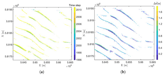
Figure 11.
Model classification of the accepted, alternative models, . (a) showing the epoch at which the offset was identified and (b) the size of the corresponding offset, .
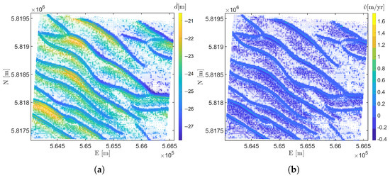
Figure 12.
Estimated parameters of the final model selection: (a) Estimated depth, and (b) Estimated slope, .
The results of nodal trends exemplified in Figure 10 also seem to correspond well with a migrating sandwave passing those locations. This is also suggested in Figure 13 where an example of cross-sections through a sandwave feature is extracted in the direction of maximum variability in sub-area NF for the different, available epochs. This was done using a 5 m × 5 m gridded DEM for simplicity. The nodal trends of the observations, extracted for different x-locations (local coordinate system) show similar trends as for the models selected in Figure 10. This indicates that the testing procedure developed resulted in selected models that can detect a correct identification of the spatial and temporal change in depths. This then implies that the selected models can be used for predicting the changes in depths, which is described further in Section 4.
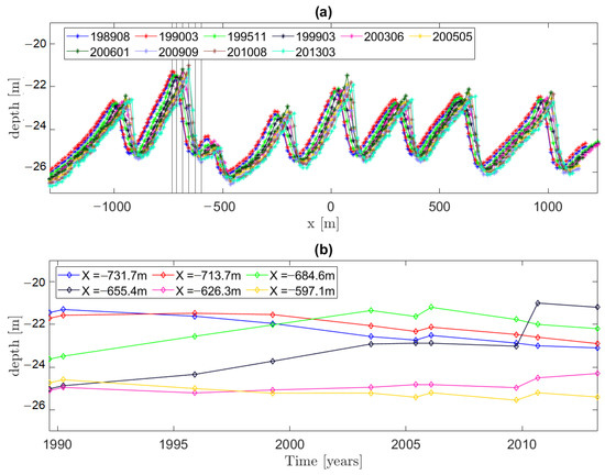
Figure 13.
Example of temporal change in sand wave feature. (a) Cross-sections for different epochs and (b) Nodal temporal trend of the observations for different x-locations shown by the vertical, black lines in (a).
4. Prediction Using the Models Selected: Area NF
Using the most likely models or estimators that were selected using the method outlined in Section 2.4, a prediction with associated uncertainties can be obtained for area NF for , two years from the last survey moment. The predictive performance of the selected models were evaluated and the results for the for the sub-area NF as defined in Equation (28) was 0.23 m. Figure 14 shows the relationship between the predicted variables, depth, and the predicted slope at predicted time where the variability of is greater for the nodes that accept an model, and where values are on average somewhat smaller than that of the nodes for which the model was accepted.
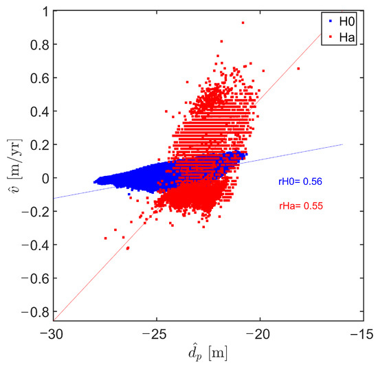
Figure 14.
Relationship between predicted variables using accepted and models, where and gives the respective correlation coefficients.
Using the models that are accepted, we present the spatial results for the prediction at , for a projection of 2 years after the last epoch, . The difference in the depths between the last epoch, and is computed as :
and presented as a difference map in meters in Figure 15a. To account for the direction and magnitude of the change in depth, a negative change indicates that the trend in the depths is becoming shallower and a positive change indicates the depths are becoming deeper.
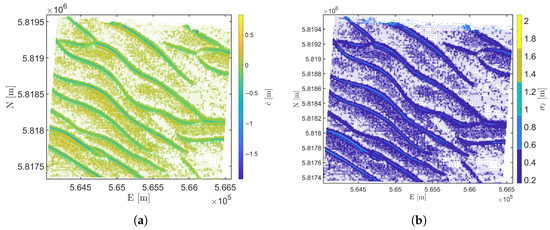
Figure 15.
Area NF showing results of (a) and (b) .
The variance of can be determined using the variance-covariance matrix as:
The main diagonal of in Equation (25) contains the variances and of the parameters . The uncertainties and propagate to where is the square root of the variance, or standard deviation of as shown in Figure 15b. Figure 15b therefore shows the order of magnitude of the quality of the estimated , where the less precise estimates of are predominantly located near the crests of the sandwave features (with the exception of very few larger values in the northern edges where the length of the times series can be shorter, refer to Figure 8a due to the subdivision of the defined areas during the preprocessing step as described in Section 3.1). These locations are consistent with where the alternative piecewise linear models, are being accepted in favour of the nominal model, , account for 7% of the total number of nodes and are considered critical locations for the safety of navigation. Recall that the piecewise linear models, can detect larger changes in depth where the second segment of the model and estimated parameters, and are used for the prediction. Hence, the larger estimated slope parameter and the relatively smaller number of original observations used in the second line segment of the model as compared to the nominal model , introduce larger uncertainties in predicted depth value, . However, increasing the length of the original time series when more surveys become available can improve the precision of and hence the estimated .
Additionally, the does not provide information on the probability that will be smaller or greater than a certain value. Here the concept of confidence intervals or regions can be used [32]. Given parameter , and as the user-defined level of significance, the confidence interval is defined as:
where gives the distance from which the estimated will be from the true value with a confidence level of [32]. Such a confidence interval is often denoted as where commonly used intervals are the and i.e., the and confidence intervals, respectively. This concept is further explained and applied in the following Section 5 where is used at the indicator variable to evaluate the probabilities of exceeding a particular threshold value.
5. Risk-Alert Indicator and Decision Thresholds
In this section, we introduce the problem of estimating the probability that an indicator variable, (in this case per node, j for a sub-area) will cross an upper and lower decision threshold. This choice of threshold level serves as the basis for determining risk-alert levels using quality indicators as a tool for decision-making when determining the next time of resurvey.
Under the assumption that the estimators selected for the prediction follow a Gaussian distribution, the confidence interval for a given choice of , denoted as a user-specified probability, can be computed. This provides information on the predicted probability that is smaller or larger than an upper and lower, threshold value, :
Using Equation (32), the confidence interval is defined. The or significance level is often set to so that the associated confidence interval is . This implies that the predicted will be within a distance of with a confidence level of , as in Equation (32). The choice of used is for the confidence interval. The upper threshold is defined as and the lower threshold as to distinguish between a shoaling and a deeper respectively.
Advanced geostatistical techniques allow the uncertainty of the estimation to be expressed in terms of risk where [40,41,42] used Disjunctive Kriging and other research used an Indicator Kriging approach based on [43] for evaluating the probability, given the observations, that the indicator variable exceeds a critical threshold. This research contribution of developing a risk-alert indicator uses a simple count of the nodes of the indicator variable where it crosses a decision threshold using the same sub-area of interest, NF. The confidence represent the interval that includes the true with a probability of . Varying the value of the for the corresponding changes the decision threshold at which the probability of is crossing the upper and lower threshold values.
Values for are provided by the NLHS as a guide for negative changes in depth (i.e., shoaling depths and the respective decision thresholds for risk-alerts regarding safety of navigation) for different depth ranges as in Table 3.
Table 3.
Decision thresholds provided as a guide by the NLHS with specific focus on safety of navigation.
An example of estimated probabilities is shown in Figure 16 at the confidence interval for upper and lower threshold values set to [−0.1 m 0.2 m] and [−0.5 m 0.2 m] respectively, where the lower threshold value is kept constant here for comparison and absence of user guidelines. The black and red nodes tend to occur in clusters, suggesting the spatial correlation with the areas that are shoaling and becoming deeper as a result of the shape of sandwave features and its migration.
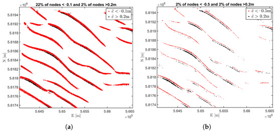
Figure 16.
Vulnerable nodes at the 95% confidence interval for predefined decision thresholds. (a) presents the predicted probability at 95% confidence level using [0.2 m < < −0.1 m] and (b) Predicted probability at 95% confidence level using [0.2 m < < −0.5 m].
To evaluate other applications such as pipelines and cables on the seafloor, stricter threshold levels may be needed. As the first steps towards determining the upper and lower decision thresholds per sub-area, a range of threshold values for is incorporated and evaluated per node for sub-area NF, shown in Figure 17.
Figure 17.
Estimated probability at 95% confidence level using a range of upper and lower decision thresholds.
The estimation of the probabilities, the choice of the indicator variable used and the adaptable decision thresholds, need to be further evaluated. This will be done to further evaluate the use of the uncertainty of the predictions and hence the approach towards delimiting categorical risk-levels for survey areas of different seafloor dynamics.
6. Conclusions
An adaptable approach using time series of bathymetry data and a combination of the OMT statistic and the GLRT to obtain the most likely functional model for evaluating a risk-based approach towards optimisation of resurvey frequencies has been developed. Combining the OMT statistic and the GLRT improves the selection of the estimators and accuracy of detection of change in depths.
This library of functional models is built on empirical observations and consists of physically realistic characterisations of the seafloor dynamics and applied to a case study area where sandwaves are dominant, using nodal analysis (0D). The addition of piecewise linear models offers another characterisation of seafloor changes to detect and identify the trends in the nodal time series corresponding to the changes. This hypothesis testing approach ensures that the assumption for the nominal model, is empirically derived, resulting in an innovative and adaptable approach on the choice of for the hypothesis testing design and model selection procedure and reliability.
The selection of the most likely functional model allows for short term prediction in changes in seafloor depth with associated uncertainties since the results show spatial consistency where alternative models are selected. This methodology allows for the predictive values to be applied in estimation of the probabilities that the changes in seafloor depths cross an upper and lower decision threshold for the purposes of risk-alert and decision-making for determining the next resurvey moment or dredging intervention. This functional model selection procedure is also relevant to other marine engineering applications where detecting seafloor changes is critical to decision-making, such as buried cables and pipelines on the seafloor.
Future research will evaluate further the choice of additional variable indicator(s) and decision thresholds, for risk-alert assessments towards a probability map for decision-making regarding resurveys. The approach developed is applicable to areas that exhibit different seafloor dynamics and when different types of remote sensing data are used or combined. The research contribution in general, is not limited to the use of seafloor depth data.
Author Contributions
Conceptualization, R.T. and S.V.; methodology, R.T. and S.V.; validation, R.T. and A.D.; formal analysis, R.T.; investigation, R.T. and S.V.; resources, R.T. and S.V.; data curation, R.T. and S.V.; writing—original draft preparation, R.T. and S.V.; writing—review and editing, R.T. and S.V.; visualization, R.T.; supervision, S.V.; project administration, S.V.; funding acquisition, S.V. All authors have read and agreed to the published version of the manuscript.
Funding
This project was part of the larger multidisciplinary SMARTSEA project (number 13275) entitled ’Safe Navigation by optimising seabed monitoring and waterway maintenance using fundamental knowledge for seabed dynamics’ which was partly financed by the Netherlands Organisation for Scientific Research (NWO). The data used for this research was provided by the Netherlands Hydrographic Service, Rijkswaterstaat and Deltares.
Institutional Review Board Statement
Not applicable.
Informed Consent Statement
Not applicable.
Data Availability Statement
The data used for this research was provided by the Netherlands Hydrographic Service, Rijkswaterstaat and archived by Deltares. Data and further information regarding access to data source can be found at https://publicwiki.deltares.nl/display/OET/Dataset+documentation+bathymetry+NLHO (accessed in June 2018).
Conflicts of Interest
The authors declare no conflict of interest.
Abbreviations
The following abbreviations and symbols are used in this manuscript:
| 0D | Zero-dimensional |
| 1D | One-dimensional |
| 2D | Two-dimensional |
| BAS | Bathymetric Archive System |
| BLUE | Best Linear Unbiased Estimation |
| DEM | Digital Elevation Model |
| DGPS | Differential Global Positioning System |
| DIA | Detection, Identification and Adaptation |
| DOF | Degrees of Freedom |
| GLRT | Generalised Likelihood Ratio Test |
| GPS | Global Positioning System |
| IMO | International Maritime Organisation |
| InSAR | Interferometric Synthetic Aperture Radar |
| LAT | Lowest Astronomical Tide |
| LOOCV | Leave-One-Out Cross-Validation |
| MBES | Multibeam Echosounding |
| NCS | Netherlands Continental Shelf |
| NLHS | Netherlands Hydrographic Service |
| OMT | Overall Model Test |
| RWS | Rijkswaterstaat |
| SA | Selective Availability |
| SBES | Single-Beam Echosounding |
| SOLAS | Safety of Life at Sea |
| UTM | Universal Traverse Mercator |
| WGS84 | World Geodetic System 1984 |
| dispersion | |
| expectation | |
| error distribution of simulated observation (Section 2.5) | |
| decision threshold value (Section 5) | |
| probability of incorrectly accepting an alternative hypothesis or | |
| ’level of significance’ | |
| power of test | |
| residuals | |
| adjusted observations | |
| estimated unknown parameters | |
| difference in depth | |
| reference depth of the last survey | |
| ∇ | vector of additional unknown parameters for alternative hypothesis |
| average period between surveys | |
| standard deviation | |
| depth variance | |
| MBES error variance | |
| spatial variance | |
| kriging variance | |
| standard deviation threshold | |
| azimuth East of North | |
| depth observables | |
| random measurement errors | |
| Test statistic with q degrees of freedom | |
| predicted depth | |
| A | design matrix |
| a | acceleration |
| parameters of IHO S44 standards for depth uncertainty | |
| C | specification matrix of alternative hypothesis |
| mean cross-validation error | |
| d | depth parameter |
| seafloor characterisation in time | |
| null hypothesis | |
| alternative hypothesis | |
| i | number of hypotheses; model number |
| j | node index |
| J | total number of nodes |
| k | critical value |
| m | number of observations; number of hypotheses per grid node |
| m | meter |
| M | model |
| N | number of observations per grid cell |
| n | number of unknown parameters; total number of epochs |
| number of piecewise models | |
| p | position; subscript for predicted value (Section 2.5) |
| q | degrees of freedom |
| precision of prediction | |
| precision of the estimator | |
| variance matrix of the observations | |
| R | test ratio |
| r | correlation coefficient |
| S | last survey moment |
| next expected survey | |
| t | time; vector of survey moments |
| v | slope parameter |
| x | unknown parameters (Section 2) |
| Easting and Northing position | |
| simulated observation |
References
- IHO Standards for Hydrographic Surveys. Special Publication No. 44, 6th ed.; Technical Report; International Hydrographic Bureau: Monaco, 2020. [Google Scholar]
- Rijkswaterstaat. Dutch Standards for Hydrographic Surveys. Rijkswaterstaat. 3.0 ed. 2009. Available online: https://puc.overheid.nl/rijkswaterstaat/doc/PUC_158368_31/ (accessed on June 2020).
- McCave, I.N. Sand waves in the North Sea off the coast of Holland. Mar. Geol. 1971, 10, 199–225. [Google Scholar] [CrossRef]
- Nemeth, A.A.; Hulscher, S.J.M.H.; de Vriend, H.J. Modelling sand wave migration in shallow shelf seas. Cont. Shelf Res. 2002, 22, 2795–2806. [Google Scholar] [CrossRef]
- Terwindt, J.H.J. Sand waves in the Southern Bight of the North Sea. Mar. Geol. 1971, 10, 51–67. [Google Scholar] [CrossRef]
- Knaapen, M.A.F. Sandwave Migration Predictor based on shape information. J. Geophys. Res. Earth Surf. 2005, 110, 1–9. [Google Scholar] [CrossRef]
- Dorst, L. Estimating Sea Floor Dynamics in the Southern North Sea to Improve Bathymetric Survey Planning. Ph.D. Thesis, University of Twente, Enschede, The Netherlands, 2009. [Google Scholar] [CrossRef]
- Van Dijk, T.A.G.P.; Van der Tak, C.; De Boer, W.P.; Kleuskens, M.H.P.; Doornenbal, P.J.; Noorlandt, R.P.; Marges, V.C. The Scientific Validation of the Hydrographic Survey Policy of the Netherlands Hydrographic Office, Royal Netherlands Navy; Technical Report; Deltares: Delft, The Netherlands, 2011. [Google Scholar]
- Besio, G.; Blondeaux, P.; Brocchini, M.; Vittori, G. On the modeling of sand wave migration. J. Geophys. Res. Ocean. 2004, 109. [Google Scholar] [CrossRef]
- Lindenbergh, R. Parameter estimation and deformation analysis of sand waves and mega ripples. In Proceedings of the 2nd International Workshop on Marine Sand Wave and River Dune Dynamics, Enschede, The Netherlands, 1–2 April 2004. [Google Scholar]
- Pluymaekers, S.; Lindenbergh, R.; Simons, D.; de Ronde, J. A Deformation Analysis of a Dynamic Estuary Using Two-Weekly MBES Surveying. In OCEANS 2007-Europe; Institute of Electrical and Electronics Engineers: Aberdee, UK, 2007; pp. 1–6. [Google Scholar] [CrossRef]
- Huizenga, B. The Interpretation of Seabed Dynamics on the Netherlands Continental Shelf. Master’s Thesis, Delft University of Technology, Delft, The Netherlands, 2008. [Google Scholar]
- Lindenbergh, R.; Hanssen, R. Eolian deformation detection and modeling using airborne laser altimetry. In Proceedings of the IGARSS 2003, IEEE International Geoscience and Remote Sensing Symposium, Toulouse, France, 21–25 July 2003; pp. 1–4. [Google Scholar] [CrossRef]
- Chang, L.; Hanssen, R.F. A Probabilistic Approach for InSAR Time-Series Postprocessing. IEEE Trans. Geosci. Remote Sens. 2016, 54, 421–430. [Google Scholar] [CrossRef]
- Teunissen, P.J.G. Testing Theory; Delft University Press: Delft, The Netherlands, 2000. [Google Scholar]
- Teunissen, P.J.G.; Simons, D.G.; Tiberius, C.C.J.M. Probability and Observation Theory; TU Delft: Delft, The Netherlands, 2009. [Google Scholar]
- Knaapen, M.A.F.; Hulscher, S.J.M.H. Regeneration of sand waves after dredging. Coast. Eng. 2002, 46, 277–289. [Google Scholar] [CrossRef]
- Irish, J.L.; White, T.E. Coastal engineering applications of high-resolution lidar bathymetry. Coast. Eng. 1998, 35, 47–71. [Google Scholar] [CrossRef]
- Brusch, S.; Held, P.; Lehner, S.; Rosenthal, W.; Pleskachevsky, A. Underwater bottom topography in coastal areas from TerraSAR-X data. Int. J. Remote Sens. 2011, 32, 4527–4543. [Google Scholar] [CrossRef]
- Casal, G.; Hedley, J.D.; Monteys, X.; Harris, P.; Cahalane, C.; McCarthy, T. Satellite-derived bathymetry in optically complex waters using a model inversion approach and Sentinel-2 data. Estuar. Coast. Shelf Sci. 2020, 241, 106814. [Google Scholar] [CrossRef]
- Niroumand-Jadidi, M.; Bovolo, F.; Bruzzone, L. SMART-SDB: Sample-specific multiple band ratio technique for satellite-derived bathymetry. Remote Sens. Environ. 2020, 251, 112091. [Google Scholar] [CrossRef]
- Sagawa, T.; Yamashita, Y.; Okumura, T.; Yamanokuchi, T. Satellite Derived Bathymetry Using Machine Learning and Multi-Temporal Satellite Images. Remote Sens. 2019, 11, 1155. [Google Scholar] [CrossRef]
- Dorst, L. Survey plan improvement by detecting sea floor dynamics in archived echo sounder surveys. Int. Hydrogr. Rev. 2004, 5, 1–15. [Google Scholar]
- Samet, H. An Overview of Quadtrees, Octrees, and Related Hierarchical Data Structures. In Theoretical Foundations of Computer Graphics and CAD; Earnshaw, R.A., Ed.; Springer: Berlin/Heidelberg, Germany, 1988; pp. 51–68. [Google Scholar] [CrossRef]
- Toodesh, R.; Verhagen, S. Adaptive, variable resolution grids for bathymetric applications using a quadtree approach. J. Appl. Geod. 2018, 12, 311–322. [Google Scholar] [CrossRef]
- Wackernagel, H. Multivariate Geostatistics: An Introduction with Applications; Springer: Berlin/Heidelberg, Germany; New York, NY, USA, 2003. [Google Scholar]
- Van Dijk, T.; Kleuskens, M.H.P.; Dorst, L.L.; Van der Tak, C.; Doornenbal, P.J.; Van der Spek, A.J.F.; Hoogendoorn, R.M.; Rodriguez Aguilera, D.; Menninga, P.J.; Noorlandt, R.P. Quantified and applied sea-bed dynamics of the Netherlands Continental Shelf and the Wadden Sea. In Proceedings of the Jubilee Conference Proceedings, NCK-Days 2012: Crossing Borders in Coastal Research, Enschede, The Netherlands, 13–16 March 2012. [Google Scholar]
- Calder, B. On the uncertainty of archive hydrographic data sets. J. Ocean. Eng. IEEE 2006, 31, 249–265. [Google Scholar] [CrossRef]
- Hare, R.; Eakins, B.; Amante, C. Modelling bathymetric uncertainty. Int. Hydrogr. Rev. 2011, 6, 1–30. [Google Scholar]
- Chiles, J.P.; Delfiner, P. Geostatistics: Modeling Spatial Uncertainty; Wiley Series in Probability and Statistics; Applied Probability and Statistics Section; Wiley: New York, NY, USA, 1999. [Google Scholar]
- Digipol, G. Rijkwaterstaat, Rijkstituut voor Kust en Zee, The Hague, The Netherlands; Technical Report; Rijkswaterstaat: Utrecht, The Netherlands, 2007. [Google Scholar]
- Verhagen, S.; Teunissen, P.J.G. Least-Squares Estimation and Kalman Filtering. In Springer Handbook of Global Navigation Satellite Systems; Teunissen, P.J.G., Montenbruck, O., Eds.; Springer International Publishing: Cham, Switzerland, 2017; pp. 639–660. [Google Scholar] [CrossRef]
- Tukey, J.W. We Need Both Exploratory and Confirmatory. Am. Stat. 1980, 34, 23–25. [Google Scholar] [CrossRef]
- Van Dijk, T.A.G.P.; Lindenbergh, R.C.; Egberts, P.J.P. Separating bathymetric data representing multiscale rhythmic bed forms: A geostatistical and spectral method compared. J. Geophys. Res. Earth Surf. 2008, 113. [Google Scholar] [CrossRef]
- Guillen, J. Atlas of Bedforms in the Western Mediterranean; Springer: Cham, Switzerland, 2016. [Google Scholar]
- Velsink, H. The Elements of Deformation Analysis: Blending Geodetic Observations and Deformation Hypotheses. Ph.D. Thesis, Delft University of Technology, Delft, The Netherlands, 2018. [Google Scholar]
- Velsink, H. On the deformation analysis of point fields. J. Geod. 2015, 89, 1071–1087. [Google Scholar] [CrossRef]
- Wong, T.T. Performance evaluation of classification algorithms by k-fold and leave-one-out cross validation. Pattern Recognit. 2015, 48, 2839–2846. [Google Scholar] [CrossRef]
- Arlot, S.; Celisse, A. A survey of cross-validation procedures for model selection. Stat. Surv. 2010, 4, 40–79. [Google Scholar] [CrossRef]
- Goovaerts, P.; Webster, R.; Dubois, J.P. Assessing the risk of soil contamination in the Swiss Jura using indicator geostatistics. Environ. Ecol. Stat. 1997, 4, 49–64. [Google Scholar] [CrossRef]
- Webster, R.; Oliver, M.A. Optimal interpolation and isarithmic mapping of soil properties. VI. Disjunctive kriging and mapping the conditional porbability. J. Soil Sci. 1989, 40, 497–512. [Google Scholar] [CrossRef]
- Armstrong, M.; Matheron, G. Disjunctive kriging revisited: Part I. Math. Geol. 1986, 18, 711–728. [Google Scholar] [CrossRef]
- Journel, A.G. Nonparametric estimation of spatial distributions. J. Int. Assoc. Math. Geol. 1983, 15, 445–468. [Google Scholar] [CrossRef]


Publisher’s Note: MDPI stays neutral with regard to jurisdictional claims in published maps and institutional affiliations. |
© 2021 by the authors. Licensee MDPI, Basel, Switzerland. This article is an open access article distributed under the terms and conditions of the Creative Commons Attribution (CC BY) license (https://creativecommons.org/licenses/by/4.0/).