Median Polish Kriging and Sequential Gaussian Simulation for the Spatial Analysis of Source Rock Data

Abstract

In this technical note, a geostatistical model was applied to explore the spatial distribution of source rock data in terms of total organic carbon weight concentration. The median polish kriging method was used to approximate the “row and column effect” in the generated array data, in order for the ordinary kriging methodology to be applied by means of the residuals. Moreover, the sequential Gaussian simulation was employed to quantify the uncertainty of the estimates. The modified Box–Cox technique was applied to normalize the residuals and a cross-validation analysis was performed to evaluate the efficiency of the method. A map of the spatial distribution of total organic carbon weight concentration was constructed along with the 5% and 95% confidence intervals. This work encourages the use of the median polish kriging method for similar applications.

1. Introduction

Onshore and coastal petroleum exploration commonly involves rock samples from different locations, geological formations and depths, which are analyzed for their mineral composition and organic properties. Geostatistics can be used to spatially analyze these properties and provide their spatial distribution in terms of mathematical principles of interdependence. In petroleum resources evaluation studies, geostatistics in the form of kriging have traditionally been used successfully [1,2,3,4,5]. Over the last decades, multi-point techniques, simulations and seismic inversion methods have been developed and successfully applied in reservoir modeling [6,7].

In this work, we present a combined methodology for spatial analysis of the distribution of total organic carbon weight concentration (TOC wt%) from rock samples. The weight percentage of organic carbon in source rocks represents the concentration of organic material. A 0.5% value by weight of TOC is the minimum allowed for an effective source rock sample. Besides, a value of 2% is considered the minimum for shale gas reservoirs. Values greater than 10% are also probable. However, such values indicate the likelihood that kerogen, rather than other types of hydrocarbons, fills the pore space [8].

The median polish method (MEP) combined with the sequentially Gaussian simulation (SGS) is applied to estimate the spatial distribution of the available dataset in an attempt to propose an alternative method to previous approaches for mapping TOC wt% [9]. In addition, it can designate areas that would be potentially under environmental risk during prospective explorations [10]. MEP approximates large scale variations by iteratively removing the median from the rows and columns of the gridded data. The determined residuals can be analyzed with the kriging method by means of the variogram to study the small-scale spatial structure variation of the study variable and to be combined with the estimated median polish trend [11,12]. MEP is widely used in geostatistical applications to overcome bias as well as the influence of extreme values [13,14], while SGS is used in geostatistical simulation applications in various disciplines [15,16,17]. However, the two methods have never been combined for a specific application, especially in the discipline of hydrocarbons. A similar work involving spatial polycyclic aromatic hydrocarbons (PAHs) analysis using indicator kriging and SGS has been successfully conducted [18], suggesting that such approaches can be useful for the spatial analysis of data related to hydrocarbons.

2. Materials and Methods

The data evaluated were from subsurface Mesozoic rock samples from the eastern onshore Gulf Coast Basin (mainly Mississippi and Louisiana), USA [19]. Specifically, 561 samples were collected by the USGS from 2011–2017 to investigate potential undiscovered petroleum resources. Part of the data from the aforementioned dataset was used in a recent study and showed that most samples were derived from a common mixed marine terrigenous source rock [20]. In this work, the determined TOC wt% was geostatistically evaluated in terms of its mean value at each sampling location. Thus, 132 unevenly distributed samples were used to perform the spatial analysis of TOC wt% in the study area (Figure 1). The sample was decomposed into trend and residuals according to the principles of MEP method. The residuals were examined to see if they followed a normal distribution, and a modification of the classic Box–Cox technique [21,22,23] was implemented to transform them.

2.1. Median Polish Kriging (MEPK)

Let $Z\left(s\right)$ be a random field of sample size $N$. A mean structure can be obtained by additive decomposition of the row and column effect to define irregular gridded spatial data in which grid spacings do not have to be equal in either the horizonal or vertical directions:

$$u\left(s_i\right)=a+r_k+c_l, s_i=\left(x_l,y_k\right)$$

(1)

where $r_k$and $c_l$are the row and column effects, respectively, and a is a constant. The nodes of an overlaid rectangular grid are allocated to the data positions if they are irregularly spaced.

A method called median polish has been proposed to estimate the additive effects given above using median theory in order to avoid bias and the impact of extreme values. [11]. Median polish is applied by recurrent mining until convergence of the row and column medians by means of a convergence criterion. It gives new estimators of $a, r_k,c_l$ which we write as $\tilde{a}, \widetilde{r_k},\widetilde{c_l}$. Thus, the initial spatial data are defined as:

$$Z\left(s_i\right)=\tilde{a}+{\tilde{r}}_k+{\tilde{c}}_l+R\left(s_i\right)$$

(2)

where $R\left(s_i\right)$ corresponds to the residual term which is trend free to consent the application of ordinary kriging (OK),

$$\tilde{R}\left(s_0\right)={\displaystyle \sum }_{i=1}^N{\mathsf{\lambda }}_i R\left(s_i\right)$$

(3)

For $s=\left(x,y\right)\text{'}$ in the area bounded by the lines that connect the four nodes: $\left(x_l, y_k\right)’$; $\left(x_{l+1}, y_k\right)’;\left(x_l, y_{k+1}\right)’$; $\left(x_{l+1}, y_{k+1}\right)’$, subject to $x_l<x_{l+1}$ and $y_k<y_{k+1},$ defines the planar interpolant,

$$\tilde{u}\left(s\right)\equiv \tilde{a}+{\tilde{r}}_k+\left(\frac{y-y_k}{y_{k+1}-y_k}\right)\left({\tilde{r}}_{k+1}-{\tilde{r}}_k\right)+{\tilde{c}}_l+\left( \frac{x-x_k}{x_{k+1}-x_k}\right) \left({\tilde{c}}_{k+1}-{\tilde{c}}_l\right)$$

(4)

Details for the corresponding extrapolation equation can be found in Martínez et al. [13].

Thus, the median polish kriging predictor is provided from Equation (5),

$$\tilde{Z}\left(s_0\right)\equiv \tilde{u}\left(s_0\right)+\tilde{R}\left(s_0\right).$$

(5)

Furthermore, the median polish kriging variance is defined by the following equation:

$${\sigma }_{MP}^2\left(s_0\right)=\gamma \text{'}{\Gamma }^{-1}\gamma -{\left(1\text{'}{\Gamma }^{-1}\gamma -1\right)}^2/\left(1\text{'}{\Gamma }^{-1}1\right)$$

(6)

where 1 is an $n\times 1$ vector of ones, $\gamma$ the variogram vector of the residuals between ${\mathbf{s}}_j$ (observation point) and ${\mathbf{s}}_0$ (estimation point). $\Gamma$ is the variogram matrix of the residuals, $\left(N_0+1\right)\times \left(N_0+1\right)$, at the observation locations [11,13]. The decomposed median predictors are not considered in the MEP variance error estimation. Therefore, to calculate the uncertainty of estimations in a reliable way, SGS is applied.

2.2. Sequential Gaussian Simulation

The sequential Gaussian simulation (SGS) is a stochastic approach for producing equiprobable realizations (maps) of spatial distribution of a variable on a grid by means of kriging methodology. SGS fundamentals are based on drawing from a collection of conditional distributions of univariate realizations. The conditional cumulative distribution function (CDF) is defined as,

$$F\left({\mathbf{s}}_1\left|N\right.\right)=F\left({\mathbf{s}}_1\left|N\right.\right)\dots F\left({\mathbf{s}}_N\left|N-1\right.\right)$$

(7)

SGS is obtained using kriging estimates, where each simulated map is a realization of a multivariate normal process. For conditional SGS, the kriging variance at sampling locations is zero to ensure that the only possible drawings are those of the sampled values. SGS is applied in terms of kriging estimator by means of a linear combination of random variables at location ${\mathbf{s}}_i$ to estimate the value at location ${\mathbf{s}}_0$ [4,18]. OK method applies that $z(s)$ and $z\in Z$ is a random function with a constant but unknown mean. The OK estimate $\widehat{z}({\mathbf{s}}_0)$ at $s_0$ is calculated based on a weighted sum of the data,

$$\widehat{z}({\mathbf{s}}_0)={\displaystyle {\sum }_{\{i: s_i\in {\mathbb{S}}_0\}}{\lambda }_i z_i({\mathbf{s}}_i)}.$$

(8)

The weights ${\lambda }_i$ depend on the variogram model ${\gamma }_z(r)$ [24] and are calculated by minimizing the mean square estimation error conditionally on the zero-bias constraint [11]. In detail, the following $(N_0+1)\times (N_0+1)$ linear system of equations provides the weights ${\lambda }_i$,

$${\displaystyle {\sum }_{\{i: s_i\in {\mathbb{S}}_0\}}{\lambda }_i }\hspace{0.17em}{\gamma }_z\hspace{0.17em}({\mathbf{s}}_i,{\mathbf{s}}_j)+\mu =\hspace{0.17em}{\gamma }_z\hspace{0.17em}({\mathbf{s}}_j,{\mathbf{s}}_0),\hspace{1em}j=1,\dots ,N_0$$

(9)

$${\displaystyle {\sum }_{\{i: s_i\in {\mathbb{S}}_0\}}{\lambda }_i }=1$$

(10)

where $N_0$ is the set of points included in the search neighborhood of ${\mathbf{s}}_0^{}$,${\gamma }_z(\hspace{0.17em}{\mathbf{s}}_i,{\mathbf{s}}_j)\hspace{0.17em}$and ${\gamma }_z(\hspace{0.17em}{\mathbf{s}}_j,{\mathbf{s}}_0)\hspace{0.17em}$ are the variograms between two observation points ${\mathbf{s}}_i$,${\mathbf{s}}_j$, and between ${\mathbf{s}}_j$ and the estimation point ${\mathbf{s}}_0$, respectively, by means of a theoretical variogram model. The term $\mu$ corresponds to the Lagrange multiplier imposing the no-bias constraint. Equation (10) implements the zero-bias condition.

Kriging methods provide the estimation of a variable $\widehat{z}({\mathbf{s}}_0)$ accompanied by the associated uncertainty, i.e., corresponding estimation’s error variance. The error variance of OK is independent of data values, is zero at monitoring locations and increases away from them, depends on the data configuration, i.e., complexity of the random field spatial variability as modeled by the variogram, while two identical spatially distant pairs of sampled points have the same variance independently of their values [25].

The SGS algorithm steps are outlined below as follows [18]:

(1)

Examine if the original data follow normal distribution and apply transformation.

(2)

A node at location $s$ is randomly selected that has not been yet simulated.

(3)

Apply kriging estimation at $\widehat{z}\left(s_0\right)$ and calculate the corresponding kriging variance $\sigma { }_E^2\left(s_0\right)$.

(4)

Draw a random value from the normal distribution $N\left(\widehat{z}\left(s_0\right), \sigma { }_E^2\left(s_0\right)\right)$, which corresponds to the simulated value.

(5)

The newly simulated value is added in the dataset and the process moves to another location.

(6)

Repeat the procedure above until there are no locations left.

(7)

If needed, back transformation to the original data scale applies to all values.

The main advantage of using geostatistical simulation is that any realization has the same variogram as the data. This is due to the sampling that applies from the conditional distribution during the simulation process [24].

2.3. Variogram

The experimental variogram of the transformed data was first calculated using the method of moments,

$${\widehat{\gamma }}_Z(r_k)=\frac{1}{2N(r_k)}\hspace{0.17em}{\displaystyle \sum _{i,j=1}^{N(r_k)}\left\{{\left[Z(s_i)-Z(s_j)\right]}^2\right\}\hspace{1em}}$$

(11)

where $N(r_k)$ denotes the number of point pairs within class $r_k$. The theoretical variogram fit was held using the Spartan variogram function considering the model parameters $\theta \hspace{0.17em}$,

$${\gamma }_Z(r; \hspace{0.33em}\theta )=C_Z(0; \hspace{0.33em}\theta )-C_Z(r; \hspace{0.33em}\theta )$$

(12)

The Spartan function is defined as follows [22,26,27]:

$$C_Z(h; \mathsf{\theta })=\left\{\begin{array}{l}\frac{{\eta }_0 e^{-h{\beta }_2\hspace{0.17em}}}{2\pi \sqrt{ |{\eta }_1^2-4|}}\left[\frac{\sin (h{\beta }_1)}{h{\beta }_1}\right], \hspace{1em}\mathrm{for} \left|{\eta }_1\right|<2,\hspace{0.33em}\hspace{0.17em}{\sigma }_z^2=\frac{{\eta }_0}{2\pi \sqrt{ |{\eta }_1^2-4|}}\\ \frac{{\eta }_0 e^{-h\hspace{0.17em}}}{8\pi },\hspace{1em}\mathrm{for} {\eta }_1=2,\hspace{0.33em}\hspace{0.17em}{\sigma }_z^2=\frac{{\eta }_0}{8\pi }\hspace{1em}\\ \frac{{\eta }_0 (e^{-h{\omega }_1\hspace{0.17em}}-e^{-h{\omega }_2\hspace{0.17em}})}{4\pi ({\omega }_2-{\omega }_1) h\sqrt{ |{\eta }_1^2-4|}}, \hspace{1em} \mathrm{for} {\eta }_1>2,\hspace{0.33em}\hspace{0.17em}{\sigma }_z^2=\frac{{\eta }_0}{4\pi \sqrt{ |{\eta }_1^2-4|}}\hspace{0.17em}\end{array}\right.$$

(13)

where ${\eta }_0$ is the scale factor, ${\eta }_1$ is the rigidity coefficient, ${\beta }_1={\left|2-{\eta }_1\right|}^{1/2}/2$ is a dimensionless wavenumber, ${\beta }_2={\left|2+{\eta }_1\right|}^{1/2}/2$ and ${\omega }_{1,2}={\left(\left|{\eta }_1\mp \Delta \right|/2\right)}^{1/2}$, $\Delta ={\left|{\eta }_1^2-4\right|}^{1/2}$, $h=r/\xi$ is the normalized lag vector, $\xi$ is the correlation length, $h=\left|h\right|$ is the distance norm and ${\sigma }_z^2$ is the variance. The Spartan family models depending on ${\eta }_1^{}$coefficient values have a characteristic wave behavior near the sill that can capture important increments or decrements of the experimental variogram values. Therefore, this characteristic can provide optimum fitting.

The geostatistical analysis using the proposed methods and tools was performed in Matlab^® environment developing original codes.

2.4. Cross-Validation

The proposed method performance is assessed using a leave one out cross-validation procedure. The estimated values are compared with the corresponding observations using a series of performance metrics. The bias error, the mean absolute error and the linear correlation coefficient were examined:

Bias (optimum value close to 0, positive or negative sign denotes overestimation or underestimation):

$${\epsilon }_{BIAS}=\frac{1}{N}{\displaystyle {\sum }_{i=1}^N}\widehat{z}(s_i)-z(s_i)$$

(14)

Mean absolute error (MAE) (optimum value close to 0):

$${\epsilon }_{\mathrm{MA}}=\frac{1}{N}{\displaystyle {\sum }_{i=1}^N\left|\widehat{z}(s_i)-z(s_i)\right|}$$

(15)

Linear correlation coefficient (optimum value close to 1):

$$\mathrm{R}=\frac{{\displaystyle {\sum }_{i=1}^N\left[z(s_i)-\overline{z(s_i)}\right] \left[\widehat{z}(s_i)-\overline{\widehat{z}(s_i)}\right]}}{\sqrt{ {\displaystyle \sum _{i=1}^N\left[z(s_i)-\overline{z(s_i)}\right]{ }^2}}\hspace{0.17em}\sqrt{ {\displaystyle \sum _{i=1}^N\left[\widehat{z}(s_i)-\overline{\widehat{z}(s_i)}\right]{ }^2}}\hspace{0.17em}}$$

(16)

The term $\widehat{z}(s_i)$ is the estimation at point $s_i$, $z(s_i)$ the observed value, $\overline{z(s_i)}$ the spatial average of the observation data and $\overline{\widehat{z}(s_i)}$ the spatial average of the estimations [28].

2.5. Methodology Flowchart

The proposed methodological steps described previously in detail are summarized in a flowchart (Figure 2) presenting the basic steps of the combined geostatistical tools applied to provide a reliable map with the spatial distribution of TOC wt% and the relative uncertainty of estimations.

3. Results

In this technical note, we apply a robust method for generating maps of TOC wt% using non-uniformly distributed monitoring stations and consider the joint application of MEPK with SGS. The sample data (Figure 3) are aligned with the nearest grid nodes according to the methodology, receiving new coordinates that correspond to the grid lines. In the case of several data aligned to a grid node, the median substitutes the data values [14].

The advantage of MEP is the robust fitting of a smooth and flexible trend surface. The MEP procedure first decomposes the data into trend and residuals, as explained in the methodology section. It then tests whether the residuals follow a normal distribution. The characteristics of the sample are shown in

Table 1. Statistical measures of TOC wt% data. $z_{\min }$: minimum value; $z_{\max }$: maximum value; $z_{0.50}$: median; $m_z$: mean; ${\widehat{\sigma }}_z$: standard deviation; ${\widehat{s}}_z$: skewness factor; ${\widehat{k}}_z$: kurtosis factor.

${\mathit{z}}_{\mathbf{min}}$	${\mathit{m}}_{\mathit{z}}$	${\mathit{z}}_{\mathbf{max}}$	${\widehat{\mathit{\sigma }}}_{\mathit{z}}$	${\widehat{\mathit{s}}}_{\mathit{z}}$	${\widehat{\mathit{k}}}_{\mathit{z}}$	${\mathit{z}}_{0.50}$
0.05 wt%	0.82 wt%	5.24 wt%	0.80 wt%	2.80	13.74	0.67 wt%

. The residuals’ skewness is equal to 1.68 and kurtosis to 4.86. Thus, TOC wt% residuals do not follow the normal distribution in order for OK and SGS to be suitable for application. Therefore, the modified Box–Cox technique [22,23] was applied to transform the residuals. The metrics are now improved to s = 0.02 and kurtosis, k = 3.26, very close to the desired Gaussian distribution metrics (s = 0 and k = 3.00). The transformed residuals’ histogram is presented in Figure 4.

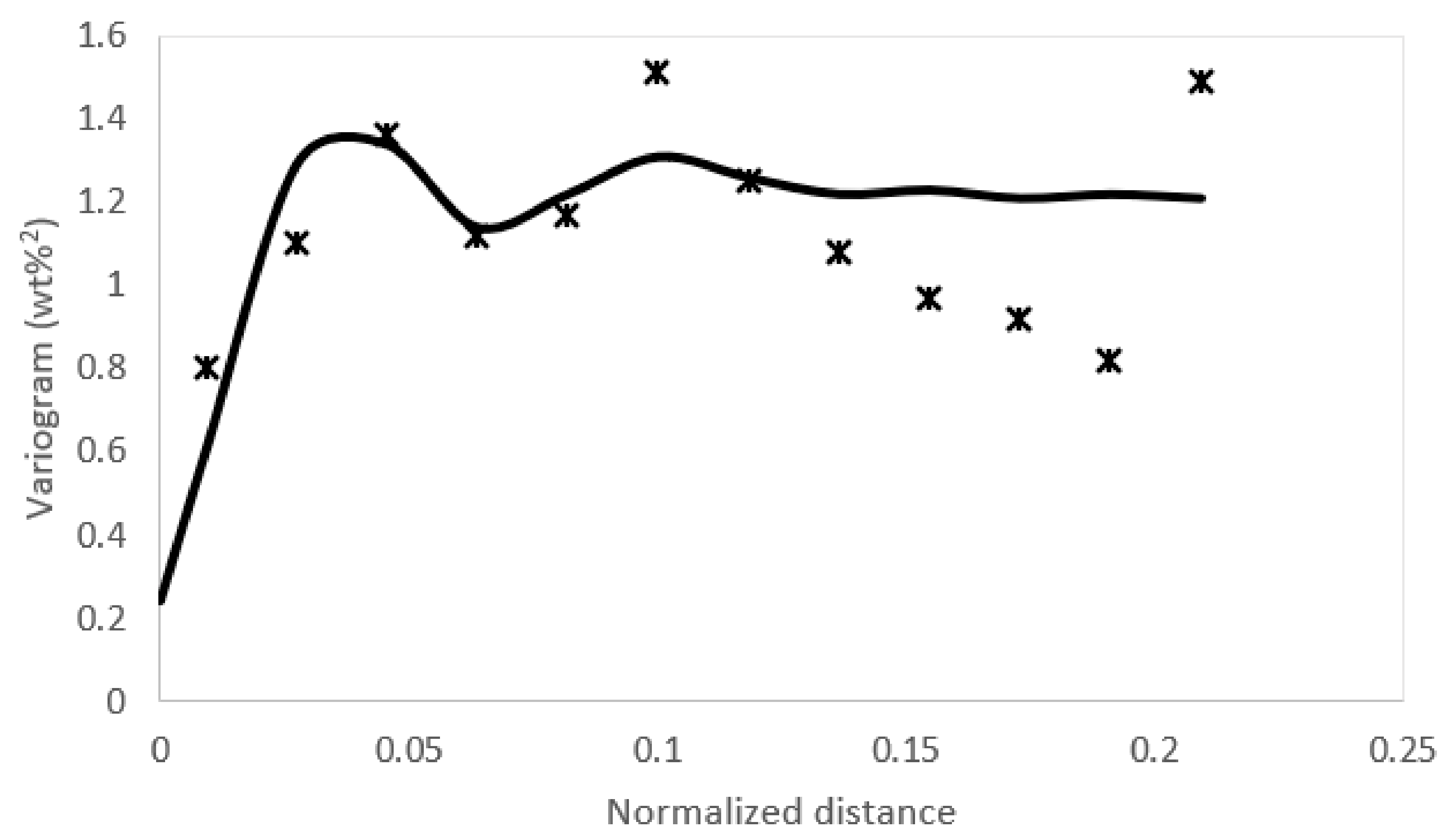
The residuals’ spatial dependence structure was fitted using the Spartan model (Figure 5). The calculated variogram parameters are ${\sigma }_z^2=1.38$, ${\eta }_1=-1.96$, $\xi =0.17$ and nugget $c=0.23$ wt%².

The MEPK method prediction error by means of cross-validation error (after back transformation of residuals) is presented in

Table 2. Leave one out cross-validation estimates of the median polish kriging method.

MAE (TOC wt%)	BIAS (TOC wt%)	R
0.10	0.03	0.94

. The cross-validation shows that errors between estimated and measured values are close to zero and significantly correlated. Thus, the method provides satisfactory estimation capability.

Furthermore, in this work, the mean of the TOC wt% simulated estimations (Figure 6) is presented from MEPK using SGS, while error maps (uncertainty) were provided using the 95% (Figure 7) and 5% (Figure 8) confidence intervals of the CDF of the simulations. The provided maps were produced after back-transforming estimations to the original scale.

The spatial analysis of the TOC wt% shows the areas of the case study that have concentrations close to 2%, taking into account the associated uncertainty, which can be further investigated employing information from petroleum geology properties. The results of this work, in comparison to previous studies that employ partial information from the same dataset [20,29], are in direct agreement in terms of the designated locations that have the highest TOC wt% potential. The data used in those works were located in the core of the measurements’ location, using geochemical and spatial analysis for hydrocarbon resources evaluation. Overall, similarly to previous works, the produced map highlights localized areas of high-quality source rock properties (TOC wt%) but of poor source rock properties on average. However, according to [29], additional work to map areas and better zones that may provide an improved potential for recoverable hydrocarbons should apply. Therefore, this work exploits the entire dataset [19], in terms of the mean TOC wt% in variable geological formations, to spatially map, by means of an efficient geostatistical methodology, the average TOC wt% potential in the study area. New locations forming zones of significant TOC wt% are presented at the south-west of the study area. Additionally, this research, compared to previous works [29], contributes, apart from the more detailed and high accuracy spatial analysis, to the uncertainty estimation of the spatial analysis by applying a simulation method that presents possible realizations of the TOC wt% providing the 5% and 95% bounds of the geostatistical method predictions uncertainty. The estimation of uncertainty can help to an integrated analysis of TOC wt% spatial distribution.

SGS is a robust stochastic simulation method that provides realizations that represent spatial patterns without smoothing effect. It exploits the capability to calculate the conditional probability of a univariate random variable given only a number of conditioning values. SGS realizations can be applied to represent all the possible spatial distribution patterns of the study variable and model the estimations uncertainty in TOC wt% evaluation.

4. Conclusions

In summary, MEPK can be characterized as a hybrid method that applies in a two-dimensional surface to estimate spatial data distribution. It combines a geostatistical approach, by means of kriging methodology, and a row and column effect analysis. This work suggests that MEPK combined with SGS can model the spatial distribution of TOC wt% and provide satisfactory estimation metrics and uncertainty quantification. The main advantage of this approach is the application of a robust trend surface based on the statistical properties of the sample. Moreover, depending on the coefficient values, the Spartan variogram model can capture important increments, or decrements, of the experimental variogram shape and provide optimum fitting. Finally, this study presents an alternative methodology for the geostatistical analysis of hydrocarbon-related spatial data.