Abstract
In inverse synthetic aperture radar (ISAR) imaging system for targets with complex motion, such as ships fluctuating with oceanic waves and high maneuvering airplanes, the multi-component quadratic frequency modulation (QFM) signals are more suitable model for azimuth echo signals. The quadratic chirp rate (QCR) and chirp rate (CR) cause the ISAR imaging defocus. Thus, it is important to estimate QCR and CR of multi-component QFM signals in ISAR imaging system. The conventional QFM signal parameter estimation algorithms suffer from the cross-term problem. To solve this problem, this paper proposes the product high order ambiguity function-modified integrated cubic phase function (PHAF-MICPF). The PHAF-MICPF employs phase differentiation operation with multi-scale factors and modified coherently integrated cubic phase function (MICPF) to transform the multi-component QFM signals into the time-quadratic chirp rate (T-QCR) domains. The cross-term suppression ability of the PHAF-MICPF is improved by multiplying different T-QCR domains that are related to different scale factors. Besides, the multiplication operation can improve the anti-noise performance and solve the identifiability problem. Compared with high order ambiguity function-integrated cubic phase function (HAF-ICPF), the simulation results verify that the PHAF-MICPF acquires better cross-term suppression ability, better anti-noise performance and solves the identifiability problem.
1. Introduction
The high-resolution inverse synthetic aperture radar (ISAR) has played an important role in civil and military fields in past decades [1]. The range-Doppler (RD) method is an effective algorithm for smooth targets in ISAR imaging system [2]. According to the Stone–Weierstrass theory [3], the radar target echo should be modeled as multi-component polynomial phase signals. For slow maneuvering targets, the echo signals should be modeled as multi-linear frequency modulation (LFM) signal. The chirp rate (CR) of LFM signal will cause the image to defocus when using RD method. Thus, the RD method is not suitable for slow maneuvering targets. To solve this problem, the CR should be estimated to remove the effect of CR. Thus, several effective LFM signal parameter estimation algorithms have been proposed, such as the fractional Fourier transform (FRFT) [4,5], the short time Fourier transform (STFT) [6], the modified Wigner–Ville distribution (MWVD) [7] and the coherently integrated cubic phase function (ICPF) [8].
For targets with high maneuvering movement, multi-component quadratic frequency modulation (QFM) signals are more accurate to describe the echo signals. The quadratic chirp rate (QCR) can also cause the image to defocus. To solve this problem, the QCR of QFM signal should also be estimated to remove the effect of QCR. Therefore, many QFM signals estimation algorithms have been proposed. The maximum likelihood (ML) [9] method and the quantification-based method [10] are among the important algorithms. They are linear parametric estimation method. Thus, there is no cross-term problem when multi-component QFM signals exist. They have good anti-noise performance. However, their huge amount of computation cost limits their application.
The cubic phase function (CPF) [11,12] estimates the parameters of QFM signal by bilinear transform and one-dimensional (1-D) maximization. Thus, it has low computation cost. However, it suffers from the cross-term problem when multi-component QFM signals exist and it has poor estimation performance under low signal-to-noise ratio (SNR). To improve the cross-terms suppression ability of CPF, the product CPF [13,14] is proposed. The product CPF improves the cross-term suppression ability by multiplying the different CPF, which is related to the delay variable. Meanwhile, the multiplication operation can also improve the anti-noise performance. However, the cross-term suppression ability and the anti-noise performance of product CPF are still poor. In [15], Igor Djurovic proposed high order ambiguity function-integrated CPF (HAF-ICPF) by combining the HAF and ICPF. This algorithm employs HAF to demodulate the QFM signal to LFM signal. Then, the QCR can be estimated by the peak of ICPF. The CR can be estimated by dechirp operation, phase differentiation operation and fast Fourier transform (FFT). The HAF-ICPF inherits good suppression ability and good anti-noise performance of ICPF. It improves the SNR threshold to −4 dB. However, several disadvantages still exist in HAF-ICPF. Firstly, the anti-noise performance of HAF-ICPF is still poor. Secondly, there is identifiability problem when multi-QFM signals have the same QCR.
In this paper, a new approach for QFM signal parameters estimation named product high order ambiguity function-modified integrated CPF (PHAF-MICPF) is proposed for multi-QFM signals. This algorithm employs a one-time phase differentiation operation that has multi-scale factors to demodulate the QFM signal to LFM signal. Then, the proposed algorithm employs the modified ICPF (MICPF) to transform the demodulated LFM signal into the time-quadratic chirp rate (T-QCR) domains, which are related to the scale factors. After the MICPF operation, the auto terms are transformed into same positions and the cross-terms are transformed into different positions on different T-QCR domains. The PHAF-MICPF can greatly suppress the energy of cross-terms while improving the energy of auto-terms by multiplying the different T-QCR domains. Therefore, the PHAF-MICPF can acquire better cross-term suppression ability and better anti-noise performance. Its SNR threshold can reach −5 dB. Besides, the PHAF-MICPF solves the identifiability problem of HAF-ICPF.
The remainder of this paper is organized as follows. In Section 2, we introduce the principle of HAF-ICPF briefly. In Section 3, we introduce the cross-term suppression ability and the problem of HAF-ICPF. In Section 4, we introduce the principle of PHAF-MICPF. The parameter selection criterion, cross-term suppression ability and the anti-noise performance are analyzed. In Section 5, we give a conclusion.
2. Brief Review of HAF-ICPF
The geometry of ISAR imaging used in this paper is based on the model in [16]. In this paper, the range alignment and the phase error are not discussed in detail. The range alignment and the phase adjustment algorithms are discussed in [7,17,18,19]. This paper only focuses on the processing of the Doppler frequency shift. The ISAR usually transmits the LFM signals. The azimuth echoes of targets with high manoeuvring movement can be described as multi-component QFM signals [20,21] after the range migration compensation and the translational-induced phase error correction.
2.1. Quadratic Frequency Modulation Signal Model
The multi-component QFM signal model can be described as follows:
where t is the slow time variable, P is the number of QFM signal components. denote the amplitude, centroid frequency (CF), CR and QCR of the ith QFM signal, respectively. is the additive complex white Gaussian noise with a mean of zero and a variance of . Next, the principle of HAF-ICPF is introduced briefly.
2.2. The Principle of HAF-ICPF
A noiseless mono-QFM signal is considered to describe the principle of HAF-ICPF. It can be described as
where A, , , and denote the amplitude, CF, CR and QCR of the mono-component QFM signal, respectively.
The HAF-ICPF employs one time phase differentiation operation to demodulate QFM signal to LFM signal. The phase differentiation can be described as
where d is the scale factor and * denotes the complex conjugation. According to [22], the scale factor d is related to the mean squared error (MSE) of QCR. Thus, it is also important for HAF-ICPF. According to the analysis of [22], the optimal scale should be set to . denotes the round up operation. N is the sampling points.
From Equation (4), we can see that QFM signal is demodulated to LFM signal after the phase differentiation operation. which is the QCR of the QFM signal becomes the CR of LFM signal. Thus, can be estimated by ICPF. Then, we use estimated to dechirp input signal. After dechirp operation, we use phase differentiation to make the dechirped signal become the sinusoidal signal whose frequency is related to . Therefore, can be estimated by FFT. From [19], we know that ICPF has good cross-term suppression ability. Thus, ICPF is the key step of HAF-ICPF. Next, we introduce the principle of ICPF.
The ICPF is defined as [15]
where is defined as [11,12]
where denotes the LFM signal. It can be described as
where and denote the CF and CR of LFM signal, respectively.
It is obvious that the peaks along the curve . From Equation (5), we can see that the ICPF also peaks along the curve . The ICPF improves cross-term suppression ability by integrating along the time variable t for CPF. By substituting Equation (4) into Equation (5), we can see that the QCR of QFM signal can be estimated by
where denotes the position of the maximum value on the T-QCR domain.
Then, the CR of QFM signal can be estimated by dechirp technique, phase differentiation operation and FFT operation. They can be described as
where is the dechirped QFM signal. denotes the estimated .
where denotes the FFT operation along the time variable t.
3. Cross-Term Suppression Performance Analysis of HAF-ICPF
From [15], we can see that HAF-ICPF has good suppression ability under most circumstances. However, there is an identifiability problem when multi-component QFM signals have the same QCR. We analyze the cross-term suppression ability and identifiability problem of HAF-ICPF in this section.
To make the problem easy to understand, we consider two noiseless component QFM signals. They can be described as
By substituting Equation (12) into Equation (3), we can obtain
where and denote auto-terms and cross-terms, respectively. They can be presented as
From Equation (15), we can see that there are cross-terms under multi-component QFM signals condition. If Equation (15) does not take the form of LFM signal, the HAF-ICPF can inherit good cross-term suppression ability of ICPF. From Equation (15), we can see that the cross-terms take the form of LFM signal when is equal to . Therefore, we can analyze the cross-term suppression ability and the identifiability problem of HAF-ICPF in three cases.
- , , .
- , , .
- , , .
where , , .
3.1. Case 1
When , , , the take the form of Equation (15). We can see that the cross-terms take the form of QFM signal. Therefore, the HAF-ICPF can suppress the cross-terms effectively under this condition.
Example 1.
Two noiseless QFM signals, and , are considered to show the cross-term suppression ability of the HAF-ICPF in this example. The sampling frequency is set to 256 Hz. The signal length N is set to 624. The scale factor d is set to 56. The parameters of and are set to , , , ; , , , and .
In Figure 1, Au1 and Au2 denote the auto-terms of and . Their positions are QCR of and . We can see that only two true peaks appear on the T-QCR domain. It is the same as the theoretical analysis. The simulation result verify that HAF-ICPF has good suppression ability under this condition.
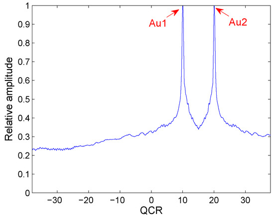
Figure 1.
Cross-term suppression of HAF-ICPF.
3.2. Case 2
When , , , the can be expressed as
From Equation (16), we can see that the cross-terms take the form of LFM signal. The will form spurious peaks after the ICPF process. Therefore, there is an identifiability problem under this condition.
Example 2.
Two noiseless QFM signals, and , are considered to show the identifiability problem of the HAF-ICPF in this example. The sampling frequency is set to 256 Hz. The signal length N is set to 624. The scale factor d is set to 56. The parameters of and are set to , , , ; , , , and .
In Figure 2, Au3 and Au4 denote the auto-terms of and . Cr1 and Cr2 denote the cross-terms. From the simulation result, we can see that the cross-terms form two spurious peaks on the T-QCR domain. Besides, the energy of spurious peaks is high enough to influence the detection of true peaks. Therefore, there is auto-term identifiability problem under this condition.
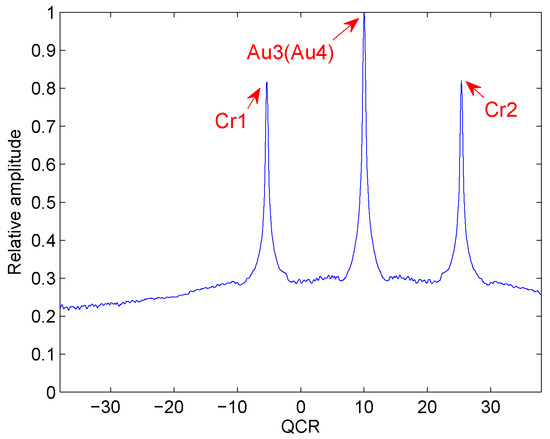
Figure 2.
Cross-term suppression of HAF-ICPF.
3.3. Case 3
When , , , the can be expressed as
From Equation (17), we can see that the cross-terms take the form of LFM signal. The will form spurious peaks after the ICPF process. The coordinates of cross-terms are . However, from Equation (13), we can see that the coordinates of auto-terms are also . Therefore, the spurious peaks will not influence the detection of true peak.
Example 3.
Two noiseless QFM signals, and , are considered to show the cross-term suppression ability of the HAF-ICPF in this example. The sampling frequency is set to 256 Hz. The signal length N is set to 624. The scale factor d is set to 56. The parameters of and are set to , , , ; , , , and .
In Figure 3, Au5 and Au6 denote the auto-terms of and . From the simulation result, we can see that the peak of Au5 and the peak of Au6 appear on the same position. It is the same as the theoretical analysis. Therefore, HAF-IPCF has good cross-term suppression ability under this condition.
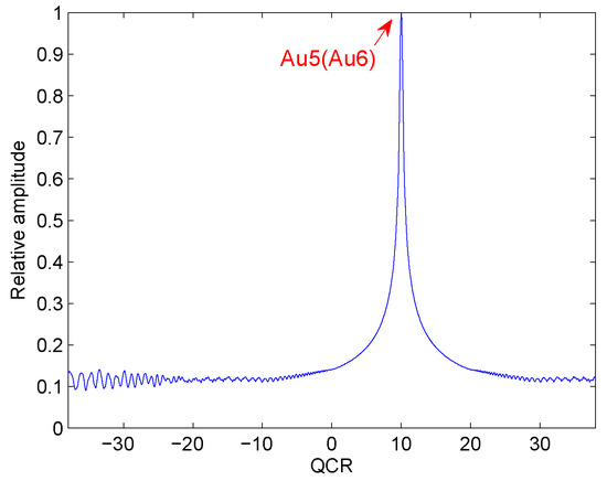
Figure 3.
Cross-term suppression of HAF-ICPF.
4. The PHAF-MICPF Method
From the analysis of Section 3, we can see that HAF-ICPF has an identifiability problem when , , . To solve the identifiability problem, we propose PHAF-MICPF. PHAF-MICPF employs phase differentiation operation with multi-scale factors to complete the order reduction. The coordinates of auto-terms are proportional to the scale factors after the ICPF process. However, the coordinates of cross-terms are not proportional to the scale factors. Therefore, PHAF-MICPF proposes the MICPF to transform the auto-terms into the same position and transform the cross-terms into the different positions on the different T-QCR domains. Then, PHAF-MICPF solves the identifiability problem and improve the cross-term suppression ability by multiplying the different T-QCR domains.
4.1. The Principle of PHAF-MICPF
The PHAF-MICPF employs phase differentiation operation with multi-scale factors to demodulate QFM signal to LFM signal. The phase differentiation operation with multi-scale factors can be described as
where denotes the set of multi-scale factors.
To introduce the principle of PHAF-MICPF, two noiseless QFM signals are considered. Substituting Equation (12) into Equation (18), we can get
The auto-terms and cross-terms can be described as
From the analysis of Section 3, we can see that the HAF-ICPF will enhance the identifiability problem when and . From Equations (20) and (21), we can see that the coordinates of auto-terms and cross-terms after the ICPF process can be described as Equations (22) and (23) when and .
From the coordinates of auto-terms, it is easy to see that they are proportional to the scale factors. The relationship between the QCR of auto-terms can be described as
However, the coordinates of cross-terms are not proportional to the scale factors. Therefore, we propose the MICPF to transform the auto-terms into the same positions and the cross-terms into different positions on different T-QCR domains, which are related to the scale factors. The process can be described as
where is the new QCR and is the reference QCR.
The PHAF-MICPF multiply different MICPF to solve the identifiability problem of HAF-ICPF. The multiplication operation can be described as
4.2. Selection of Scale Factors
From [22], the scale factors is related to the anti-noise performance. Therefore, they are important for the PHAF-MICPF. Through the analysis of [10], the optimal scale factor can help the algorithm acquire the smallest MSEs of QCR. The optimal scale factor can be described as
where N is the signal length.
From the analysis above, PHAF-MICPF can acquire the best anti-noise performance if the scale factors are all selected to the optimal ones. However, from Equation (23), we can see that the coordinates of cross-terms are proportional to scale factors when the scales factors are all selected to the optimal ones. Therefore, the scale factors should be selected to different ones. Considering the anti-noise performance and the accuracy of QCR, the sub-optimal scale factors should be selected around the optimal ones.
The number of scale factors is also important for the anti-noise performance of the algorithm. From the analysis of [22], we can see that the anti-noise performance improves with the increase of the scale factor number. However, the computation cost rapidly increases with the increase of the number of scale factors. Besides, the anti-noise performance increases slightly when the scale factor number is bigger than two. Therefore, the number of scale factors is usually selected to two.
4.3. Cross-Term Suppression Ability Analysis
Through the theoretical analysis above, we have proved that PHAF-MICPF can acquire better suppression ability and solve the identifiability problem of HAF-ICPF. In this section, we give some examples to verify that the PHAF-MICPF has better cross-term suppression ability than HAF-ICPF. Besides, it can solve the identifiability problem of HAF-ICPF.
Example 4.
Two noiseless QFM signals, and , are considered to show the cross-term suppression ability of the PHAF-MICPF when , , in this example. The scale factors of PHAF-MICPF are set to . The sampling frequency is set to 256 Hz. The signal length N is set to 624. The HAF-ICPF is also analyzed. The parameters of and are set to , , , ; , , , and .
In Figure 4, Au1 and Au2 denote the auto-terms of and . We can see that there are two true peaks appear on the T-QCR domain after the PHAF-MICPF process. It is the same as the theoretical analysis. From the simulation result, we can see that the cross-terms of PHAF-MICPF are lower than the cross-terms of HAF-ICPF. Therefore, PHAF-MICPF has better cross-term suppression ability than HAF-ICPF under this condition.
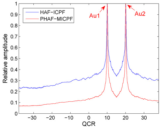
Figure 4.
Cross-term suppression of PHAF-MICPF.
Example 5.
Two noiseless QFM signals, and , are considered to show that PHAF-MICPF can solve the identifiability problem of HAF-ICPF when , , in this example.The scale factors of PHAF-MICPF are set to . The sampling frequency is set to 256 Hz. The signal length N is set to 624. The HAF-ICPF is also analyzed. The parameters of and are set to , , , ; , , , and .
In Figure 5, Au3 and Au4 denote the auto-terms of and . Cr1 and Cr2 denote the cross-terms of HAF-ICPF. Cr3, Cr4, Cr5 and Cr6 denote the cross-terms of PHAF-MICPF. The cross-terms will form the spurious peaks. From the simulation result, we can see that the energy of spurious peaks of PHAF-MICPF is very small and they can not influence the detection of true peaks. Therefore, PHAF-MICPF solves the identifiability problem of HAF-ICPF by multiplication operation.
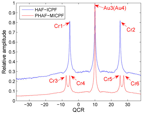
Figure 5.
Cross-term suppression of PHAF-MICPF.
Example 6.
Two noiseless QFM signals, and , are considered to show the cross-term suppression ability of the PHAF-MICPF when , , in this example. The scale factors of PHAF-MICPF are set to . The sampling frequency is set to 256 Hz. The signal length N is set to 624. The HAF-ICPF is also analyzed. The parameters of and are set to , , , ; , , , and .
From Figure 6, we can see that there is only one peak appear on the T-QCR domain after the PHAF-MICPF process. The cross-terms of PHAF-MICPF are lower than the cross-terms of HAF-ICPF. Therefore, PHAF-MICPF has better cross-term suppression ability than HAF-ICPF under this condition.
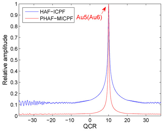
Figure 6.
Cross-term suppression of PHAF-MICPF.
To verify the good cross-term suppression ability of PHAF-MICPF more generally, we use four QFM signals as input in Example 7.
Example 7.
Four noiseless QFM signals, , , , and , are considered to show the cross-term suppression ability of the PHAF-MICPF. The scale factors of PHAF-MICPF are set to . The sampling frequency is set to 256 Hz. The signal length N is set to 624. The HAF-ICPF is also analyzed. The parameters of , , , are set to , , , ; , , , ; , , , ; , , , and .
From Figure 7, we can see that the cross-terms of PHAF-MICPF are lower than the cross-terms of HAF-ICPF. Therefore, PHAF-MICPF has better cross-term suppression ability than HAF-ICPF when there are multi-component QFM signals (more than two component QFM signals).
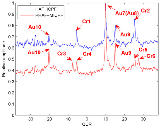
Figure 7.
Cross-term suppression of PHAF-MICPF.
From the analysis above, we can see that PHAF-MICPF has better cross-term suppression ability and solves the auto-term identifiability problem.
4.4. Anti-Noise Performance Analysis
Anti-noise performance is an important indicator to measure the effectiveness of the algorithm. Therefore, we give a simulation to evaluate the better anti-noise performance of PHAF-MICPF compared with HAF-ICPF. In this section, we use MSEs of CR and QCR to evaluate the anti-noise performance of the algorithm.
Example 8.
A noisy mono-component QFM signal is considered to evaluate the anti-noise performance of PHAF-MICPF in this example. The parameters are set to , , , . The scale factors of PHAF-MICPF are set to . The sampling frequency is set to 256 Hz. The signal length N is set to 624. The input SNR is set to [−8:1:2], and 200 trials are performed for each SNR.
In this example, HAF-ICPF is also analyzed. The MSEs of QCR and CR will increase rapidly when the input SNR is lower than certain SNR. The SNR is called the SNR threshold. It can be used to evaluate the anti-noise performance of parameter estimation algorithm. From Figure 8, we can see that the SNR threshold of PHAF-MICPF is −5 dB. It is lower than the SNR threshold of HAF-ICPF. That is because the noise of different T-QCR domains has no proportional relationship which is described as Equation (24). Thus, the multiplication operation can suppress the noise while strengthening the energy of auto-terms. Therefore, PHAF-MICPF has better anti-noise performance than HAF-ICPF.
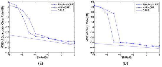
Figure 8.
Anti-noise performance analysis: (a) MSEs of QCR; and (b) MSEs of CR.
Next, we give an example to explain the influence of sub-optimal scale factors for anti-noise performance.
Example 9.
A noisy mono-component QFM signal is considered to evaluate the influence of sub-optimal scale factor for anti-noise performance in this example. The parameters are set to , , , and . The sampling frequency is set to 256 Hz. The signal length N is set to 624. The optimal scale factor is set to . The sub-optimal scale factors are set to , , and . The input SNR is set to [−8:1:2], 200 trials are performed for each SNR.
From Figure 9, we can see that the anti-noise performance is very close when the sub-optimal scale factor is selected around the optimal scale factor. However, the anti-noise performance becomes poor when the sub-optimal scale factor is selected far away the optimal scale factor. Therefore, the sub-optimal scale factor should be selected around the optimal scale factor.
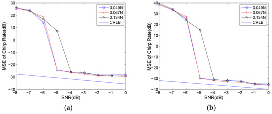
Figure 9.
Sub-optimal scale factors analysis: (a) MSEs of QCR; and (b) MSEs of CR.
5. Conclusions
In this paper, we propose the PHAF-MICPF to estimate QCR and CR of QFM signal. The PHAF-MICPF introduces phase differentiation operation with multi-scale factors to demodulate the QFM signal to LFM signal. It employs the MICPF to transform the demodulated LFM signals into the different T-QCR domains, which are related to the different scale factor. The auto-terms are transformed into the same positions and the cross-terms are transformed into the different positions on the T-QCR domains. Then, the proposed algorithm employs the multiplication operation to improve the cross-term suppression ability. The multiplication operation can also improve the anti-noise performance. Simulation results verify that PHAF-IPCF improves the cross-term suppression ability and the anti-noise performance of HAF-ICPF. Besides, PHAF-MICPF solves the auto-term identifiability problem of HAF-ICPF.
Funding
This research received no external funding.
Conflicts of Interest
The author declares no conflict of interest.
References
- Verhaelen, K.; Bauer, A.; Guenther, F.; Mueller, B.; Nist, M.; Celik, B.U.; Weidner, C.; Kuechenhoff, H.; Wallner, P. Anticipation of food safety and fraud issues: Isar-A new screening tool to monitor food prices and commodity flows. Food Control 2018, 94, 93–101. [Google Scholar] [CrossRef]
- Lulu, A.; Mobasseri, B.G. Phase matching of coincident pulses for range-doppler estimation of multiple targets. IEEE Signal Process. Lett. 2019, 26, 199–203. [Google Scholar] [CrossRef]
- Chen, X.L.; Guan, J.; Liu, N.B.; He, Y. Maneuvering target detection via radon-fractional fourier transform-based long-time coherent integration. IEEE Trans. Signal Process. 2014, 62, 939–953. [Google Scholar] [CrossRef]
- Zhao, H.R.; Qiao, L.Y.; Zhang, J.C.; Fu, N. Generalized random demodulator associated with fractional fourier transform. Circuits Syst. Signal Process. 2018, 37, 5161–5173. [Google Scholar] [CrossRef]
- Shinde, S.; Gadre, V.M. An uncertainty principle for real signals in the fractional fourier transform domain. IEEE Trans. Signal Process. 2001, 49, 2545–2548. [Google Scholar] [CrossRef]
- Hlawatsch, F.; Boudreaux-Bartels, G.F. Linear and quadratic time-frequency signal representations. IEEE Signal Process. Mag. 1992, 9, 21–67. [Google Scholar] [CrossRef]
- Xing, M.; Wu, R.; Li, Y.; Bao, Z. New isar imaging algorithm based on modified wigner-ville distribution. IET Radar Sonar Navig. 2009, 3, 70–80. [Google Scholar]
- Su, J.; Tao, H.; Rao, X.; Xie, J.; Guo, X. Coherently integrated cubic phase function for multiple LFM signals analysis. Electron. Lett. 2015, 51, 411–413. [Google Scholar] [CrossRef]
- Abatzoglou, T. Fast maximum likelihood joint estimation of frequency and frequency rate. In Proceedings of the IEEE International Conference on Acoustics, Speech, and Signal Processing (ICASSP ’86), Tokyo, Japan, 7–11 April 1986; pp. 1409–1412. [Google Scholar]
- Zheng, J.B.; Su, T.; Liu, Q.H.; Zhang, L.; Zhu, W.T. Fast parameter estimation algorithm for cubic phase signal based on quantifying effects of doppler frequency shift. Prog. Electromagn. Res. 2013, 142, 57–74. [Google Scholar] [CrossRef]
- Shea, P.O. A new technique for instantaneous frequency rate estimation. IEEE Signal Process. Lett. 2002, 9, 251–252. [Google Scholar] [CrossRef]
- Shea, P.O. A fast algorithm for estimating the parameters of a quadratic fm signal. IEEE Trans. Signal Process. 2004, 52, 385–393. [Google Scholar] [CrossRef]
- Wang, P.; Yang, J.Y. Multicomponent chirp signals analysis using product cubic phase function. Digital Signal Process. 2006, 16, 654–669. [Google Scholar] [CrossRef]
- Wang, Y.; Jiang, Y.C. Inverse synthetic aperture radar imaging of maneuvering target based on the product generalized cubic phase function. IEEE Geosci. Remote Sens. Lett. 2011, 8, 958–962. [Google Scholar] [CrossRef]
- Djurovic, I.; Simeunovic, M.; Djukanovic, S.; Wang, P. A hybrid cpf-haf estimation of polynomial-phase signals: Detailed statistical analysis. IEEE Trans. Signal Process. 2012, 60, 5010–5023. [Google Scholar] [CrossRef]
- Li, X.L.; Kong, L.J.; Cui, G.L.; Yi, W.; Yang, Y.C. Isar imaging of maneuvering target with complex motions based on ACCF-LVD. Digit. Signal Process. 2015, 46, 191–200. [Google Scholar] [CrossRef]
- Xing, M.; Wu, R.; Lan, J.; Bao, Z. Migration through resolution cell compensation in isar imaging. IEEE Geosci. Remote Sens. Lett. 2004, 1, 141–144. [Google Scholar] [CrossRef]
- Li, X.; Liu, G.; Jinlin, N. Autofocusing of isar images based on entropy minimization. IEEE Trans. Aerosp. Electron. Syst. 1999, 35, 1240–1252. [Google Scholar] [CrossRef]
- Wahl, D.E.; Eichel, P.H.; Ghiglia, D.C.; Jakowatz, C.V. Phase gradient autofocus-a robust tool for high resolution sar phase correction. IEEE Trans. Aerosp. Electron. Syst. 1994, 30, 827–835. [Google Scholar] [CrossRef]
- Bai, X.; Tao, R.; Wang, Z.; Wang, Y. Isar imaging of a ship target based on parameter estimation of multicomponent quadratic frequency-modulated signals. IEEE Trans. Geosci. Remote Sens. 2014, 52, 1418–1429. [Google Scholar] [CrossRef]
- Wu, L.; Wei, X.; Yang, D.; Wang, H.; Li, X. Isar imaging of targets with complex motion based on discrete chirp fourier transform for cubic chirps. IEEE Trans. Geosci. Remote Sens. 2012, 50, 4201–4212. [Google Scholar] [CrossRef]
- Barbarossa, S.; Scaglione, A.; Giannakis, G.B. Product high-order ambiguity function for multicomponent polynomial-phase signal modeling. IEEE Trans. Signal Process. 1998, 46, 691–708. [Google Scholar] [CrossRef]


© 2019 by the author. Licensee MDPI, Basel, Switzerland. This article is an open access article distributed under the terms and conditions of the Creative Commons Attribution (CC BY) license (http://creativecommons.org/licenses/by/4.0/).