Deep Reinforcement Learning Based Left-Turn Connected and Automated Vehicle Control at Signalized Intersection in Vehicle-to-Infrastructure Environment

Abstract

In order to solve the problem of vehicle delay caused by stops at signalized intersections, a micro-control method of a left-turning connected and automated vehicle (CAV) based on an improved deep deterministic policy gradient (DDPG) is designed in this paper. In this paper, the micro-control of the whole process of a left-turn vehicle approaching, entering, and leaving a signalized intersection is considered. In addition, in order to solve the problems of low sampling efficiency and overestimation of the critic network of the DDPG algorithm, a positive and negative reward experience replay buffer sampling mechanism and multi-critic network structure are adopted in the DDPG algorithm in this paper. Finally, the effectiveness of the signal control method, six DDPG-based methods (DDPG, PNRERB-1C-DDPG, PNRERB-3C-DDPG, PNRERB-5C-DDPG, PNRERB-5CNG-DDPG, and PNRERB-7C-DDPG), and four DQN-based methods (DQN, Dueling DQN, Double DQN, and Prioritized Replay DQN) are verified under 0.2, 0.5, and 0.7 saturation degrees of left-turning vehicles at a signalized intersection within a VISSIM simulation environment. The results show that the proposed deep reinforcement learning method can get a number of stops benefits ranging from 5% to 94%, stop time benefits ranging from 1% to 99%, and delay benefits ranging from −17% to 93%, respectively compared with the traditional signal control method.

1. Introduction

In recent years, the autonomous vehicle (AV) has attracted wide attention at home and abroad. In July 2017, BMW, Intel, and Mobileye announced their cooperation in the development of self-driving vehicles, which are expected to be officially produced in 2021 [1]. In September 2017, Baidu held an open Technology Conference on Apollo (Software platform for autonomous driving) version 1.5. In July 2018, Daimler, Bosch, and Nvidia announced the joint development of the L4 and L5 (fully autonomous driving) AVs [1]. In addition, according to KPMG’s Autonomous Vehicles Readiness Index published in 2019, the Netherlands, Singapore, and Norway ranked in the top three, while China ranked 20th [2]. However, one of the difficulties for AVs is the application at signalized intersections. Nowadays, in order to improve vehicle traffic efficiency at intersections, traffic signal control is the main form that exists universally. The application of AVs at signalized intersections is still in the research stage, especially at the beginning of AVs putting into use—that is, the mixed state of AVs and traditional human-driven vehicles (HVs), which is one of the hotspots of current research. Therefore, to design a suitable signalized intersection vehicle control method has profound theoretical and practical significance.

In order to effectively solve the problems brought by transportation, intelligent transportation systems (ITSs) have developed rapidly. The rapid development of ITS provides a lot of convenience for traffic. Vehicle-to-infrastructure (V2I) technology is one of the current development technologies of ITS. V2I technology realizes the real-time control of vehicles or roads by means of real-time communication system between vehicles and roads. Research shows that V2I technology can effectively improve vehicle safety and reduce unnecessary parking [3], or reduce fuel consumption and exhaust emissions of vehicles at intersections [4]. Besides, the development of the 5G network provides great convenience for V2I technology. The 5G network will help improve the data transmission rate between vehicles and the infrastructure. In addition, the 5G network will greatly improve the efficiency of data collection, storage, and processing for V2I [5].

However, problems are often characterized by high dimensionality and non-linearity. Deep learning (DL) and reinforcement learning (RL) can deal with this problem well and have achieved good training results in various fields [6,7]. In addition, the deep reinforcement learning (DRL) method combines the advantages of DL and RL and shows better experimental results for some problems than traditional methods (such as pure-pursuit control) [8]. At the same time, the application of DRL in traffic optimization is more extensive, such as traffic control [9,10], ramp control [11,12], AV [13], etc.

Therefore, facing complex urban road signalized intersections, considering the mixed situation of AVs and HVs, this paper designs a left-turn CAV control method of signalized intersections based on the DRL method with V2I technology. The control method proposed in this paper can provide a new control method for CAV to drive in the area of a signalized intersection.

The main contributions of this paper are as follows.

• Aiming at the micro-control problem of a left-turning CAV at a signalized intersection, a control method based on an improved deep deterministic policy gradient (DDPG) is presented in this paper. The left-turn connected and automated vehicle (CAV) approaching, inside, and leaving an intersection is integrated in the control method. In addition, unlike the current research methods of RL for vehicle control at signalized intersections, this paper controls the action of left-turn CAV as a continuous action, rather than dividing the action space into discrete action, which is more suitable for the actual situation.
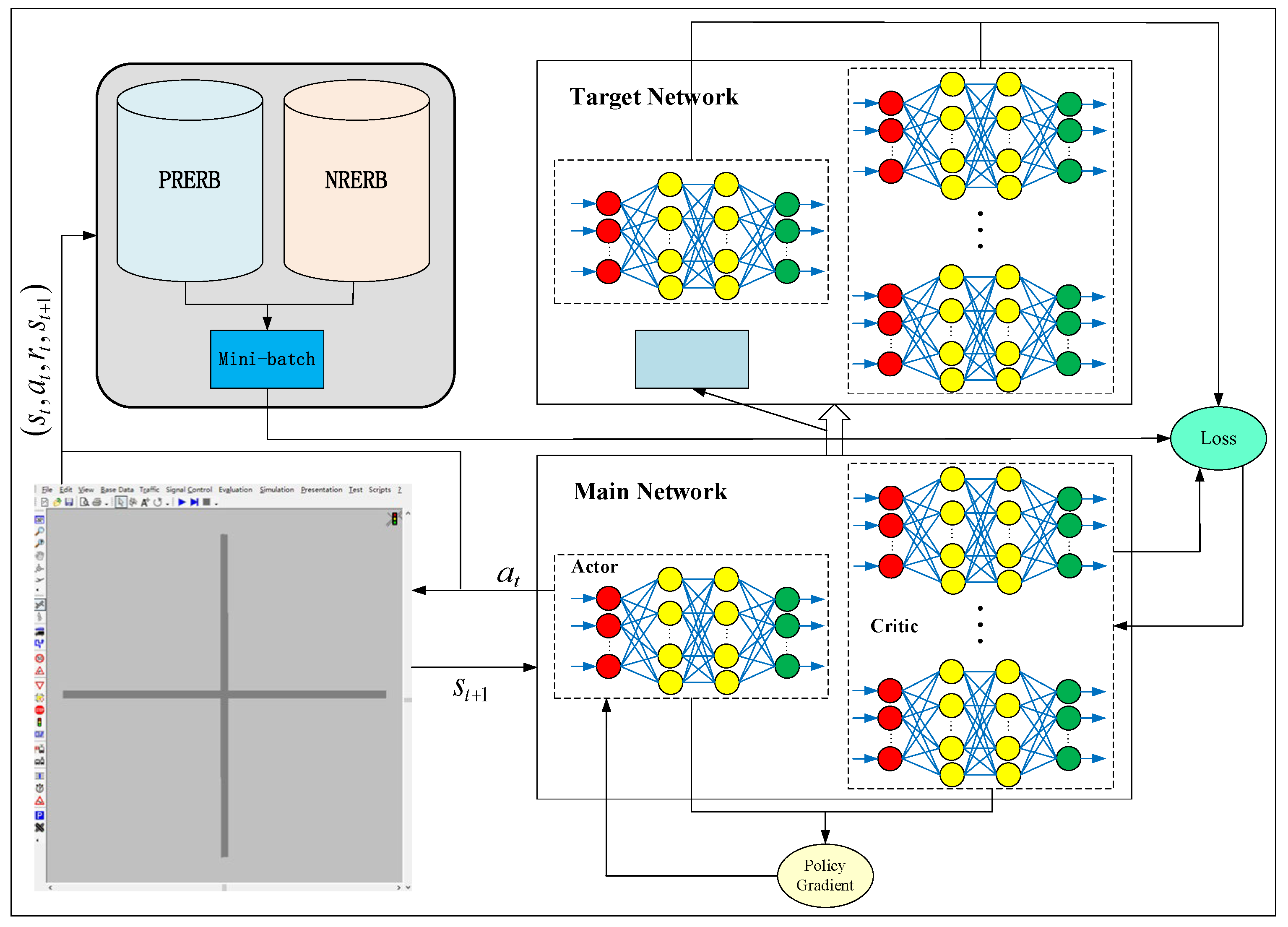
• In view of the instability of the DDPG algorithm, this paper divides the total experience replay buffer into positive reward experience replay buffer and negative reward experience replay buffer. Then, sampled from the positive negative reward experience replay buffer according to the ratio of 1:1, both excellent and not-excellent experiences can be sampled each time. At the same time, in order to avoid the overestimation of the critic network in the DDPG algorithm and accelerate the training of the actor network, the DDPG algorithm used in this paper is designed with a multi-critic structure.
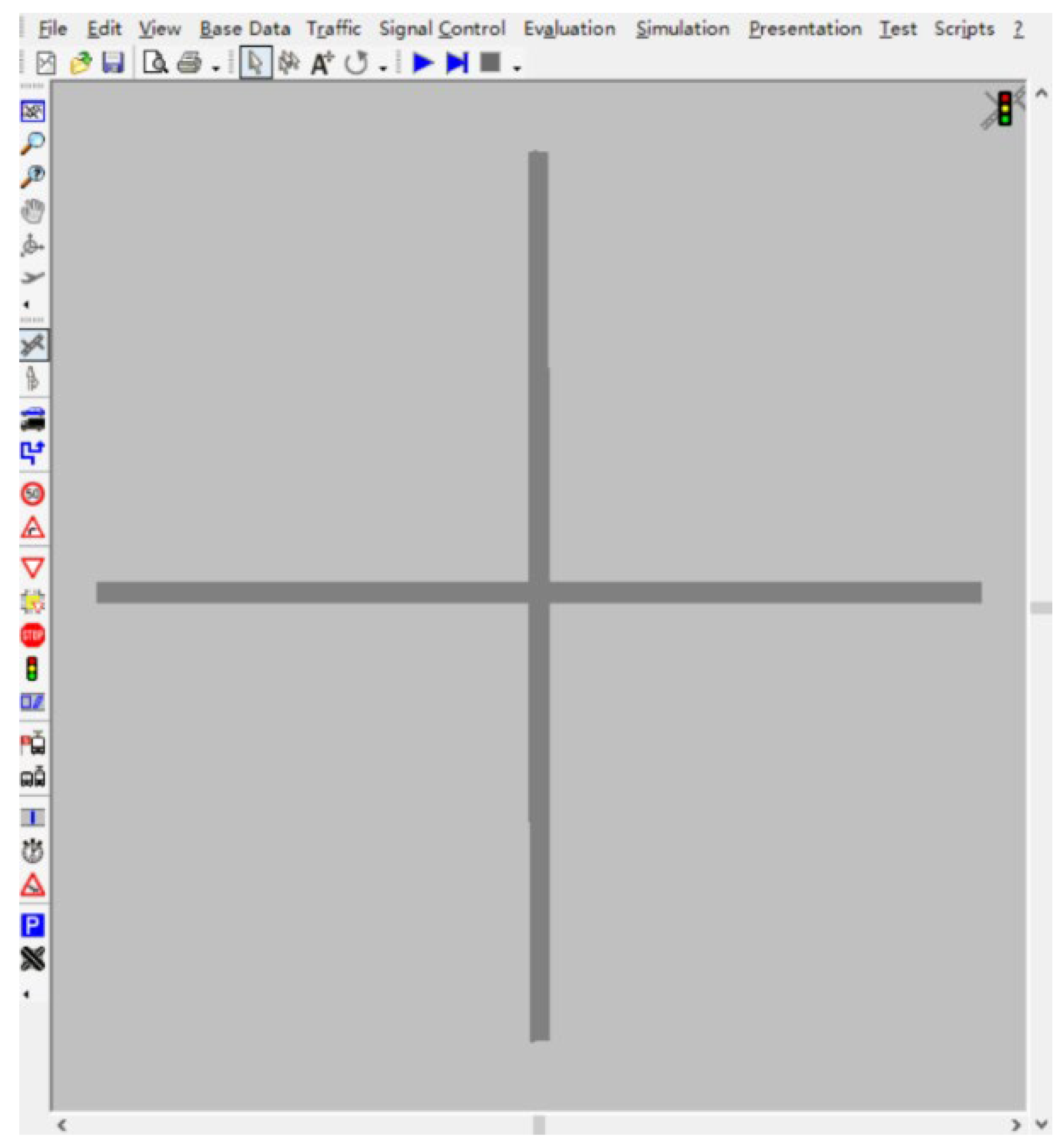
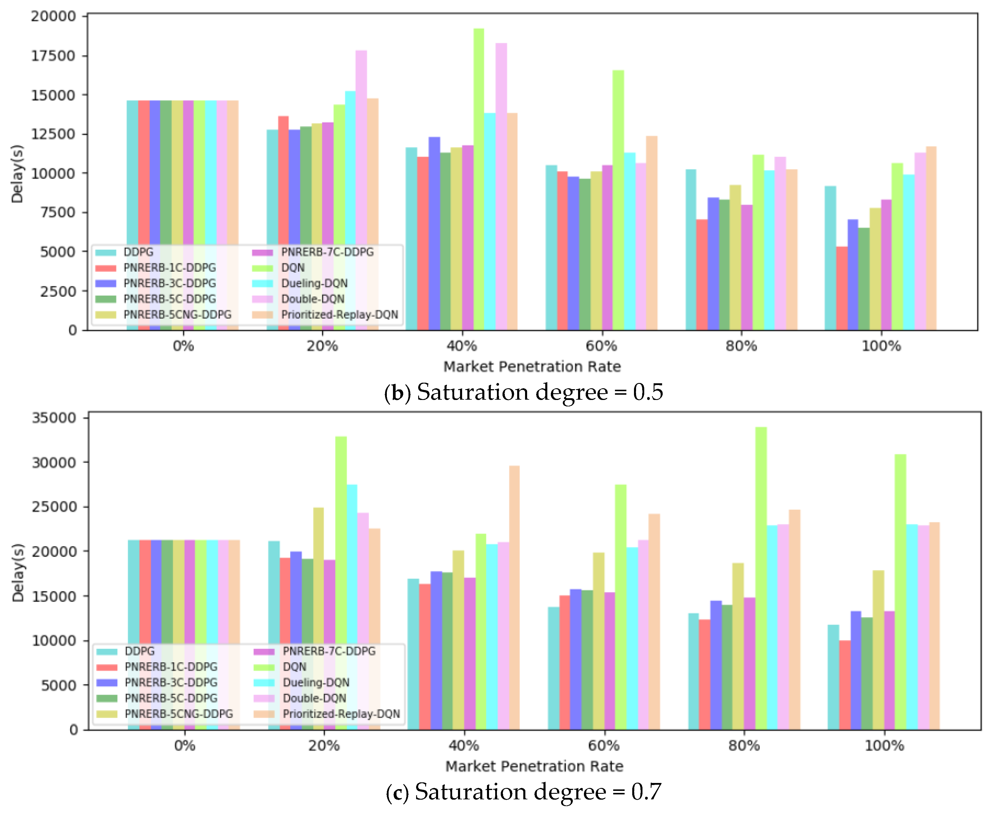
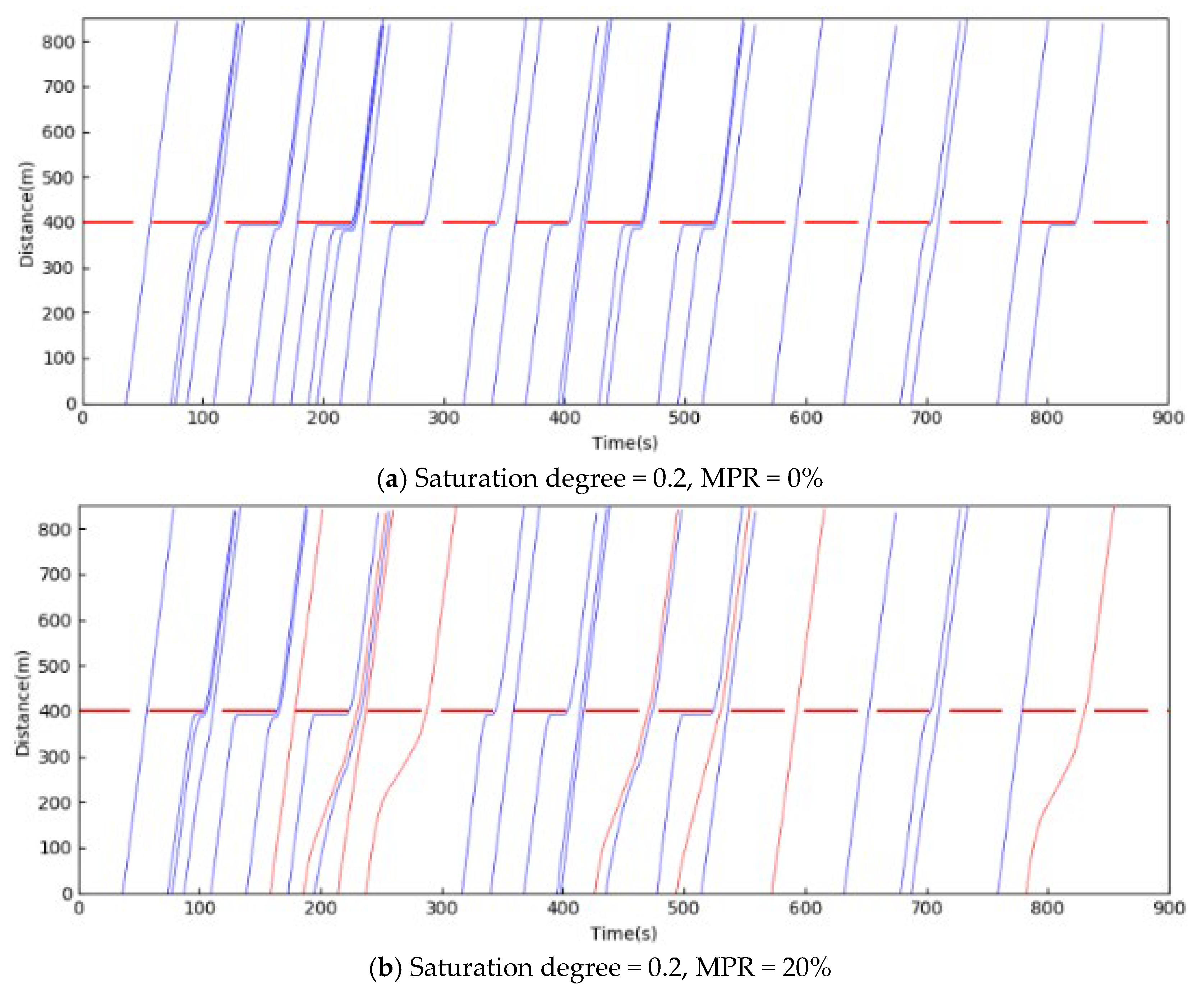
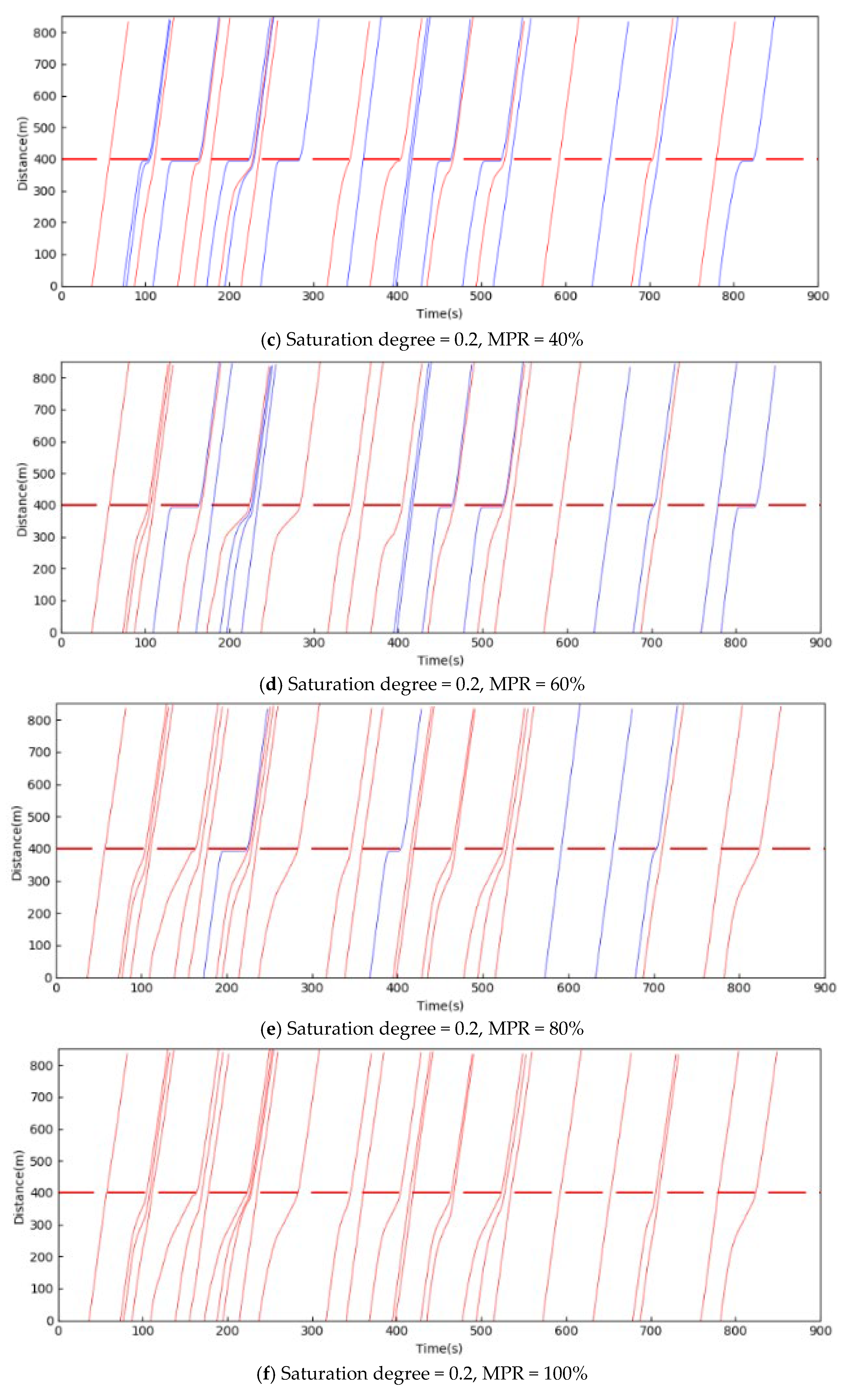
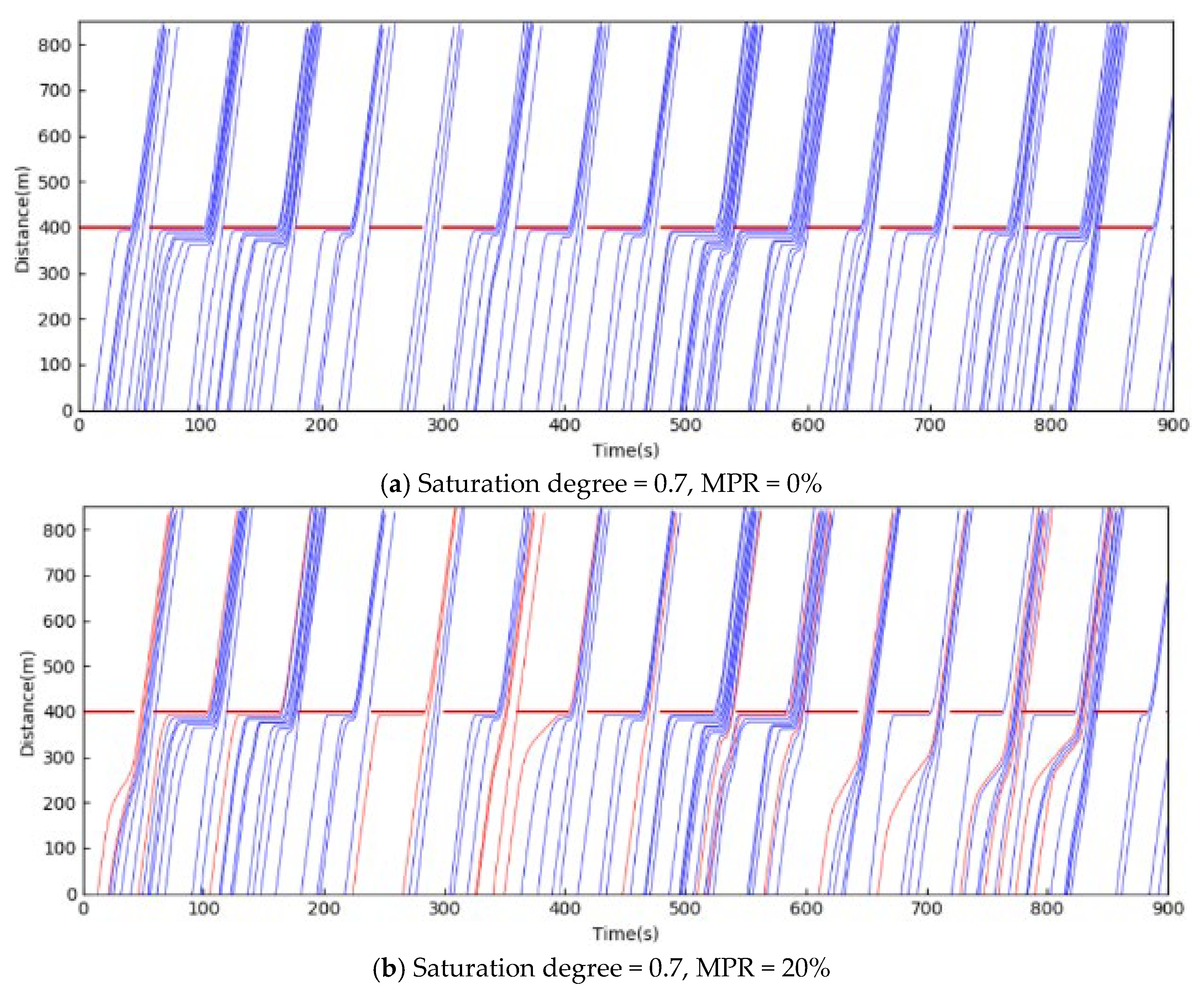
• Aiming at the problems studied in this paper, a DRL model is established. When constructing the DRL model, considering the particularity of the problem, the state of the model is processed. In addition, this paper uses micro-simulation software VISSIM to build a virtual environment and takes it as an agent-learning environment. The left-turn vehicle in the simulation environment is used as the learning agent, so that the agent can learn independently in the virtual environment. Finally, in order to verify the effectiveness of agent training in different environments, this paper analyzed the train and test results under different market penetration under 0.2, 0.5, and 0.7 saturation degrees of a signalized intersection.

The remainder of this paper is organized as follows. Section 2 summarizes the application of V2I technology in traffic, current research of signalized intersections, and RL methods. Section 3 describes the control problem and the basic assumption of the left-turn CAV under the V2I environment, as well as DRL problem. Section 4 introduces the RL methods and describes the improved DRL methods proposed in this paper. Section 5 analyzes the results. Section 6 summarizes the paper and identifies the direction of future work.

2. Literature Review

V2I can provide more safe and efficient driving information for road drivers. In the intersection area, with V2I, researchers have made a lot of contributions, whether to improve traffic safety and efficiency [14,15] or to reduce fuel consumption and exhaust emissions [16,17].

A signalized intersection is an important node in urban road traffic. Unlike continuous traffic flow on expressways, traffic flow on urban roads is often affected by intersection lights and conflicting traffic flow, resulting in increased stop time at stop lines and a large number of vehicle delays. Researchers have made a lot of research on signalized intersections, which can be divided into macro and micro fields.

In macro research, the main purpose is to optimize the traffic signal timing so that vehicles can pass through intersections safer and more efficiently [18,19]. Zhou [20] took an urban road intersection under the environment of a vehicular network as the research object and proposed an adaptive traffic signal control algorithm based on cooperative vehicle infrastructure (ATSC-CVI). Simulation results show that the algorithm has a better control effect than fixed-time control and actuated control. In order to optimize the vehicle trajectory and signalized phases at single signalized intersections in the vehicular network environment, Yu et al. [21] considered vehicles passing through intersections in a queue, and established an optimal control model for the front vehicle in the queue. Simulation results show that the proposed vehicle actuated control method has some improvements in intersection capacity, vehicle delay, and CO₂ emissions.

Micro research involves optimizing the trajectory of each vehicle to improve the overall traffic efficiency of intersections, reducing unnecessary stops, fuel consumption, and exhaust emissions [22,23]. To solve the problem of the hybrid formation of electric vehicles and traditional fuel vehicles, He and Wu [24] proposed an optimal control model. The experimental results showed that the optimal control model was beneficial to reduce the fuel consumption of the hybrid fleet. In addition, some researchers have done some research on the mixed environment of AVs and HVs. A real-time cooperative eco-driving strategy was designed for the vehicle queue of hybrid AVs and HVs by Zhao et al. [23]. They found that the proposed eco-driving strategy can effectively smooth the trajectory of fleet and reduce the fuel consumption of the whole transportation system. Gong and Du [25] proposed a cooperative queue control method for hybrid AVs and HVs, which can effectively stabilize the traffic flow of the entire queue. However, most of the research studies are from the perspective of eco-driving, aiming at reducing the fuel consumption and exhaust emissions of vehicles. In the case of mixed AVs and HVs, vehicle delays also should be taken into account. In addition, the optimization methods are mostly based on the mechanism model, and the robustness of this method is often poor.

For the study of signalized intersections, many researchers have solved the corresponding problems with the RL method. For example, by the Q-learning algorithm, Kalantari et al. [26] proposed a distributed cooperative intelligent system for AVs through intersections, which can effectively reduce the number of collisions and improve the travel time of vehicles. Shi et al. [27] applied the improved Q-learning algorithm to optimize the eco-driving behavior of motor vehicles. They found that the RL method can effectively reduce emissions, travel time, and stop time. Besides, through acquiring the real-time signal lights and location information, Matsumoto and Nishio [28] selected the best action according to the state of each time and finally optimized the driving behavior of each vehicle by using the self-learning characteristics of the RL method. Multi-agent traffic flow simulation showed that the average stop time was reduced. However, the traditional Q-learning algorithm requires a large amount of storage space to store Q tables, which is not suitable for the huge problem of state space and action space. Moreover, in practical problems, a large number of researchers only discretize the action space, not considering that many problems in reality are a problem of continuous action. The discretization of action may lead to a certain difference between the optimization result and the reality, and the reality utilization rate is low.

In addition, in order to solve the continuous action problem, Lillicrap [29] proposed a model-free algorithm, deep deterministic policy gradient (DDPG) based on deterministic policy gradients (DPGs) [30] and actor critics (AC) [31]. Unlike DRL based on the value function, the DDPG algorithm can solve the problem of continuous action space very well and has attracted extensive attention of researchers. Zuo [32] proposed a continuous RL method that combined a DDPG with human operation and applied it to the problem of AVs. The simulation results showed that this method could effectively improve the learning stability. Besides, based on DRL, Zhu [33] proposed a framework of human-like automatic driving and a car-following model. Using historical driving data as the input of RL and through the continuous trial and error of the DDPG, the DDPG can finally learn the optimal strategy. The experimental results showed that this framework structure could use many different driving environments. Undoubtedly, since the DDPG algorithm was proposed in 2015, it has attracted wide attention. However, the research related to the DDPG algorithm in the complex environment of a signalized intersection is scarce, especially in the research of AVs and HVs.

From the above literature, we can find that there are four shortcomings in the current research: firstly, because the macro research of signalized intersections is relatively early, there is more research, and there is relatively less micro research. Secondly, most of the micro research is based on the mechanism model, and the robustness of this method is poor. Furthermore, there is a lack of exploration and application of other methods (such as the DRL method). In addition, the application of RL in traffic is mainly based on discrete action RL methods, while the application of RL methods for continuous action is less. Finally, DRL has been studied in signalized intersections, but there is far more macro research than micro research. Moreover, most micro-studies mainly focus on a part of signalized intersections, lacking comprehensive consideration of the whole.

In view of the above four shortcomings, from the perspective of the micro-control of signalized intersections, this paper considers vehicle control in the whole process of approaching, moving inside, and departing from an intersection. In addition, for the micro-control problem in this paper, the DDPG algorithm is used to solve the continuous action problem. In order to further improve the performance of the algorithm, this paper adopts a DDPG method based on positive and negative reward experience replay buffer and a multi-critic structure. Finally, the virtual simulation environment is built with the micro-simulation software VISSIM, and the simulation vehicle is taken as the agent. The agent learns independently under different vehicle saturation and different CAV penetration rates, and the final optimization results are analyzed.

3. Problem Description

The problem description in this section is mainly divided into two parts. In the first part, it describes the left-turn CAV control problem in the V2I environment, which mainly describes the practical problems to be solved in this paper. In the second part, the real problems are described by the DRL method, and the model of the DRL method in this paper is established.

3.1. Description of the Left-Turning CAV Control Problem in V2I Environment

The intersection studied in this paper is a two-way multi-lane single signalized intersection, as shown in Figure 1.

The research problem in this paper can be described as follows: this paper only considers the whole process of left-turn vehicles passing through the intersection. Therefore, this paper will elaborate the problem from the perspective of left-turn vehicles. As shown in Figure 1, assume a CAV $Veh$ enters the intersection from the left lane of the west entrance road. Then, check whether the $Veh$ enters the control area of the intersection through the $Detecto{r}^1$, and send the vehicle number to the road side unit (RSU); at the same time, the $Veh$ also sends vehicle information to the RSU. Since this paper considers the coexistence of HVs and CAVs, therefore, only CAVs can send vehicle information. The RSU determines the control vehicle information through the detector information and the vehicle information sent by CAV and activates the control center system. The controlled vehicle hands over control of the vehicle to the control center system until the vehicle passes through the $Detecto{r}^2$ on the north exit. CAVs, the RSU, and the control center conduct information interaction through the V2I system [34].

In order to specify the research object, the following assumptions are made in this paper:

(1)

Within the control range, vehicles are not allowed to turn around, overtake, change lanes, etc.

(2)

Each vehicle has determined the exit road before entering the control area of the intersection.

(3)

Communication devices are installed in the CAV and RSU to ensure real-time communication between the vehicle, RSU, and the control center.

(4)

There is no communication delay or packet loss between the CAV, RSU, and control centers.

(5)

The CAV drives in full accordance with the driving behavior of the central control system.

3.2. Deep Reinforcement Learning Problem Description

3.2.1. State Description

The state space can be described as the following equation:

$$s_t=[x_t,y_t,v_t,x_t^b,y_t^b,v_t^b,si{g}_t]$$

(1)

where $s_t$ represents the current control vehicle state at time $t$; $x_t$ represents the position of the current control vehicle at time $t$ on the horizontal axis of the coordinate axis (m); $y_t$ represents the position of the current control vehicle at time $t$ on the vertical axis of the coordinate axis (m); $v_t$ represents the current control vehicle speed at time $t$ (km/h); $x_t^b$ represents the position of the front vehicle closest to the current control vehicle at time $t$ on the horizontal axis of the coordinate axis (m); $y_t^b$ represents the position of the front vehicle closest to the current control vehicle at time $t$ on the vertical axis of the coordinate axis (m); $v_t^b$ represents the speed of the nearest vehicle in front of the current control vehicle at time $t$ (km/h); $si{g}_t$ represents the left turn control signal time in the direction of east and west at time $t$(s).

(1) State processing method

Since the dimensions of location information and speed information in this paper are different, the variables of location information (including the control vehicle and the vehicle in front of the control vehicle) are divided by 10 in this paper in order to avoid the influence of big data over small data. In addition, this paper sets the speed of the traditional vehicle to the maximum expected speed. In order to avoid the influence of the CAV caused by a HV at the red light of a signal, the information of the first CAV that did not pass the stop line is temporarily adjusted during the red light. The location of the vehicle ahead is adjusted for the current CAV 10 meters ahead with a speed adjustment to 10 km/h. The same controller is used from the time when the CAV enters the control area to the time when it leaves the control area. However, the signal information has no effect on the vehicle after the CAV passes the stop line. The variable of the signal for the vehicle passing the stop line is taken as a large value of $\psi$ in this paper.

3.2.2. Action Description

The action space can be described as following equation:

$$a_t=[0,70]$$

(2)

Here, $a_t$ represents the optional action for agent at time $t$. The action is defined as the speed of the controlled vehicle (km/h) in this paper. The action space is continuous; that is, any integer between 0 km/h and 70 km/h can be taken.

3.2.3. Reward Function Description

The reward function can be described as following equation:

$$r_t=\{\begin{array}{c}{\omega }_1\cdot (d_t-d_{t-1})-{\omega }_2\cdot {\xi }_1\cdot mo{e}_t^g\begin{array}{cc}& v_t>v_m\end{array}\\ -{\xi }_2\cdot mo{e}_t^g\begin{array}{cc}& v_t\le v_m\end{array}\end{array}$$

(3)

Here, $r_t$ represents the immediate reward value for the currently controlled vehicle at time $t$. $d_t$ represents the total travel distance of the currently controlled vehicle at time $t$(m). $d_{t-1}$ represents the total travel distance of the currently controlled vehicle at time $t-1$ (m). $mo{e}_t^g$ [35] represents the instantaneous fuel consumption rate (l/s) or pollutant emission rate (mg/s) of the controlled vehicle at time $t$. $g$ represents the measured value type, including fuel consumption and carbon dioxide. It is carbon dioxide in Formula (3). ${\omega }_1$ and ${\omega }_2$ represent the weighting factor, whose units are all 1. To adjust the magnitude of the carbon dioxide emission rate, give a parameter ${\xi }_1$, whose unit is $(\mathrm{m}\cdot \mathrm{s})/\mathrm{m}\mathrm{g}$. $v_m$ represents the acceptable minimum speed (km/h). In order to prevent the current control vehicle from driving at a low speed, a penalty ${\xi }_2$ is designed, whose unit is $(\mathrm{m}\cdot \mathrm{s})/\mathrm{m}\mathrm{g}$.

The general idea of the reward function is that the control vehicle is given a penalty value when the control vehicle drives at a low speed. This is because when the vehicle speed is too low, it may cause a traffic jam situation. When the controlled vehicle drives at an acceptable speed, the efficiency of the vehicle is taken as the first goal (travel distance per second is considered). The exhaust emission of the vehicle is taken as the second goal.

4. Multi-Critic DDPG Method Based on Positive and Negative Reward Experience Replay Buffer

4.1. Reinforcement Learning

The essence of the RL [36] method is that an agent interacts with the environment through a series of trial-and-error processes, so that agents can independently execute actions in the face of a specific state, so as to get the maximum return. RL is developed by Markov decision processes (MDP), which can be expressed as a five-tuple; that is, $\left\{S,A,P,R,\gamma \right\}$. $S$ represents a finite set of states. $A$ represents a finite set of actions. $P=S\times A\times S\to [0,1]$ represents a state transition model. $R=S\times A$ represents an immediate reward function. $\gamma$ represents a discount factor [37].

4.2. Multi-Critic DDPG Method Based on Positive and Negative Reward Experience Replay Buffer (PNRERB-MC-DDPG)

At present, a large number of researchers have applied DDPG to solve many problems of continuous action space. However, there are still some problems in the application of the DDPG algorithm. The experience replay mechanism proposed in paper [38] refers to defining an experience replay buffer first. The historical experience of each interaction between the agent and the environment is stored in the experience replay buffer, and the learning data is extracted from the experience replay buffer every time. When sampling in the experience replay buffer, the selected historical experience is obtained by random selection, so it is difficult to balance the ratio of good and bad rewards, resulting in the algorithm having poor stability. In addition, the critic network plays an important role in evaluating the actions of the actor network, and an inaccurate evaluation may lead to slow convergence of the actor network. While in the learning process of the critic network, it is easy to cause the problem of overestimation, resulting in the poor learning effect of the actor network.

Therefore, the method adopted in this paper will be described in detail below:

(1) Positive and negative reward experience replay buffer (PNRERB)

Experience in an original DDPG replay buffer mix excellent and not excellent experiences. According to the positive and negative immediate reward value, the reward function designed in this paper obtains 0 reward experience seldom, and 0 reward experience is classified as a positive reward experience in the algorithm used in this paper, in which experience can be divided into positive and negative experience rewards. The positive and negative experiences are stored in the positive and negative experience replay buffer. As with the original DDPG approach, this paper initializes the size of the two experience replay buffers, and when they are full of experience, it replaces the oldest stored experience with the new historical experience. In addition, this paper adopts the method of small batch learning to train the DRL network. Therefore, the agent interacts with the environment firstly, collecting a certain amount of historical experience, and then extracting the experience from experience replay buffer to train the neural network. Each time the experience is extracted from the experience replay buffer, positive and negative reward experiences are respectively extracted from the experience replay buffer in a 1:1 ratio, so that good and bad experiences can be learned at the same time in each training network.

(2) Multi-critic network

The main network has a great influence on the whole DDPG algorithm. The critic network in the DDPG algorithm may have the problem of overestimation. While the critic network evaluation is not accurate, it is easy to cause incorrect guidance for the actor network learning. In order to reduce the overestimation problem of the critic network, Wu et al. [39] proposed a multi-critic network approach to solve the continuous problem and tested the effect of the improved algorithm in the OpenAI Gym platform. However, they just tested some simple questions, and it was not used to solve practical problems. In this paper, the multi-critic DDPG method proposed in paper [39] is combined with PNRERB to realize PNRERB-Multi-Critic-DDPG(PNRERB-MC-DDPG) methods, which are finally applied to solve the problem of signal intersection vehicle micro-control.

Since there are many networks in the critic network, it is necessary to consider the local error and the global error when calculating the loss of the critic network, so that the main network can be updated and evaluated better.

Equations (4)–(15) are used to update the network parameters.

$$L({\theta }_h)=\frac{1}{B}{\displaystyle {\sum }_i{((r_i+\gamma {Q^{\prime }}_h(s_{i+1},{\mu }^{\prime }(s_{i+1}|{\theta }^{{\mu }^{\prime }})|{\theta }_h^{Q^{\prime }}))-Q_h(s_i,a_i|{\theta }_h^Q))}^2}$$

(4)

$$L(\theta )=\frac{1}{B}{{\displaystyle {\sum }_i(y_i-Q_{avg}(s_i,a_i|\theta ))}}^2$$

(5)

$$L(p)=\frac{1}{B}{\displaystyle {\sum }_i(Q_h(s_i,a_i|{\theta }_h^Q)-Q_{avg}(s_i,a_i|\theta ))}$$

(6)

$$L={\phi }_{1}L({\theta }_h)+{\phi }_{2}L(\theta )+\varphi L(p)$$

(7)

$$y_i=r_i+\gamma {Q^{\prime }}_{avg}(s_{i+1},{\mu }^{\prime }(s_{i+1}|{\theta }^{{\mu }^{\prime }})|{\theta }^{\prime })$$

(8)

$$Q_{avg}(s_i,a_i|\theta )=\frac{1}{H}{\displaystyle {\sum }_{h=1}^H(Q_h(s_i,a_i|{\theta }_h^Q))}$$

(9)

Here, $L({\theta }_h)$ represents the loss of the critic network and its corresponding target network under the main network. $L(\theta )$ represents the error between the Q mean of the main network of multi-critics and the Q mean of the target network. $L(p)$ represents the error between each critic network in the main network and the Q mean value of target network. $L({\theta }_h)$ and $L(p)$ represent the local errors. $L(\theta )$ represents the global error. $B$ represents the learning batch. $i$ represents the batch $i$ of experience data. ${Q^{\prime }}_h(s_{i+1},{\mu }^{\prime }(s_{i+1}|{\theta }^{{\mu }^{\prime }})|{\theta }_h^{Q^{\prime }})$ represents the target value obtained by the $h$th $(h=1\dots H)$ critic network under the target network parameter ${\theta }_h^{Q^{\prime }}$, with state $s_{i+1}$ and policy ${\mu }^{\prime }$ obtained by the actor network as the input of the target network. $H$ represents the total number of critic networks. $Q_h(s_i,a_i|{\theta }_h^Q)$ represents the state action value function obtained by the $h$th critic network under the parameter ${\theta }_h^Q$. $Q_{avg}$ and ${Q^{\prime }}_{avg}$ represent the average $Q$ value of the critic network and $Q^{\prime }$ value of the target network obtained by multiple main networks, respectively. ${\phi }_1$, ${\phi }_2$ and $\varphi$ represent the weighting factor.

According to the average state action value function obtained by Formula (9), the strategy gradient is calculated by following equation:

$$\begin{array}{ll}J({\mu }_{{\theta }^{\mu }})& ={\displaystyle {\int }_S{\rho }^{\mu }(s){\mu }_{{\theta }^{\mu }}(s)Q_{avg}(s,a|\theta ){|}_{a={\mu }_{{\theta }^{\mu }}(s)}ds}\\ & =E_{s\sim {\rho }^{\mu }}[{\mu }_{{\theta }^{\mu }}(s)Q_{avg}(s,a|\theta ){|}_{a={\mu }_{{\theta }^{\mu }}(s)}]\end{array}$$

(10)

$$\begin{array}{cc}{\nabla }_{{\theta }^{\mu }}J({\mu }_{{\theta }^{\mu }})& ={\displaystyle {\int }_S{\rho }^{\mu }(s){\nabla }_{{\theta }^{\mu }}{\mu }_{{\theta }^{\mu }}(s){\nabla }_a{Q}_{avg}(s,a|\theta ){|}_{a={\mu }_{\theta }{}^{\mu }(s)}ds}\\ & =E_{s\sim {\rho }^{\mu }}[{\nabla }_{{\theta }^{\mu }}{\mu }_{{\theta }^{\mu }}(s)\nabla Q_{avg}(s,a|\theta ){|}_{a={\mu }_{\theta }{}^{\mu }(s)}]\end{array}$$

(11)

Here, ${\rho }^{\mu }(s)$ represents the state transition probability.

Finally, the calculated loss and policy gradient are used to update each critic network and actor network, respectively. For the target network update, this paper adopts the method of “soft update”. In the processing of the update, since there are multiple critic networks, the update of the target network corresponds to their respective critic networks, while the actor network has only one network. So, the update formula is:

$${\theta }_h^Q\leftarrow {\theta }_h^Q+\alpha \ast {\nabla }_{{\theta }_h^Q}L({\theta }_h^Q)$$

(12)

$${\theta }^{\mu }\leftarrow {\theta }^{\mu }+\beta \ast {\nabla }_{{\theta }^{\mu }}J({\mu }_{{\theta }^{\mu }})$$

(13)

$${\theta }_h^{Q^{\prime }}\leftarrow \tau {\theta }_h^Q+(1-\tau ){\theta }_h^{Q^{\prime }}$$

(14)

$${\theta }^{{\mu }^{\prime }}\leftarrow \tau {\theta }^{\mu }+(1-\tau ){\theta }^{{\mu }^{\prime }}$$

(15)

Here, $\alpha$ represents the learning rate of the critic network, $\beta$ represents the learning rate of the actor network, and $\tau$ represents the soft update factor of the target network.

Figure 2 shows the interaction between the PNRERB-MC-DDPG method and the environment. In this paper, the VISSIM simulation environment is used as the environment. The interactive process is as follows. Firstly, the current state is obtained from the VISSIM simulation, and the state is taken as the input to the actor network and critic network of the main network. After that, the current moment action is obtained from the actor network of the main network. Then, the action is applied to the vehicle in the VISSIM simulation environment to get the state of the next moment and the current immediate reward. At the same time, the states, actions, and rewards are stored in the experience replay buffer. Experience will be stored in either the positive reward experience replay buffer (PRERB) or negative reward experience replay buffer (NRERB). After a certain amount of experience data is stored in the experience replay buffer, the experience is extracted from it at a certain frequency. Finally, the parameters in the target network are updated in the way of a soft update until the algorithm converges. Algorithm 1 is the pseudo-code of the PNRERB-MC-DDPG method for the actual traffic problem.

Algorithm 1 PNRERB-MC-DDPG method

Step 1: Initialize the $H$ critic network $Q_h(s,a|{\theta }_h{}^Q)$ and actor network $\mu (s|{\theta }^{\mu })$ of the main network, give parameters ${\theta }_h{}^Q$ and ${\theta }^{\mu }$.

Step 2: Initialize the $H$ critic network ${Q^{\prime }}_h(s,a|{\theta }_h{}^{Q^{\prime }})$ and actor network ${\mu }^{\prime }(s|{\theta }^{{\mu }^{\prime }})$ of the target network, give parameters ${\theta }_h{}^{Q^{\prime }}\leftarrow {\theta }_h{}^Q$ and ${\theta }^{{\mu }^{\prime }}\leftarrow {\theta }^{\mu }$.

Step 3: Initialize PRERB $R^{+}$, NPERB $R^{-}$, mini-batch $B$, discount factor $\gamma$, the learning rate of critic network $\alpha$, the learning rate of the actor network $\beta$, pretraining size $PT$, noise $N$, noise reduction rate $\epsilon$, training time $T$, and random probability value $c$.

Step 4: Infinite loop

Step 5:  If there is no CAV in the current network

Step 6:    If the maximum cycle time $T$ is reached, stop.

Step 7:    If the $Detecto{r}^1$ detects the entry of the vehicle, add the vehicle number, and use the random probability to determine whether the vehicle is a CAV.

Step 8:    If the $Detecto{r}^2$ detects a vehicle leaving, remove the vehicle number.

Step 9:    Judge whether there are CAVs at present. If there is (there is a CAV ID stored in the RSU), enter line 10; otherwise, step by step simulation and jump back to Step 6.

Step 10:  If there are CAVs in the current network

Step 11:    Gets the current states of each CAV $s_t^m$

Step 12:    Infinite loop

Step 13:      If the maximum cycle time $T$ is reached, stop.

Step 14:      Select actions based on the current policy and exploration noise $$a_t^m=\mu (s_t^m|{\theta }^{\mu })+N_t.$$

Step 15:      Execute action $a_t^m$; then, get the immediate reward value $r_t^m$ and the next state $s_{t+1}^m$.

Step 16:      For the current network of all CAVs

Step 17:        if $r_t\ge 0$

Step 18:          Put experience $(s_t^m,a_t^m,r_t^m,s_{t+1}^m)$ into $R^{+}$

Step 19:        else

Step 20:          Put experience $(s_t^m,a_t^m,r_t^m,s_{t+1}^m)$ into $R^{-}$

Step 21:      If the number of experiences in $R^{+}$ is greater than $PT$

Step 22:        $N_t=N_t*\epsilon$

Step 23:        Sample data $(s_t,a_t,r_t,s_{t+1})$ were randomly selected from $R^{+}$ and $R^{-}$

Step 24:        Set $y_i=r_i+\gamma {Q^{\prime }}_{avg}(s_{i+1},{\mu }^{\prime }(s_{i+1}|{\theta }^{{\mu }^{\prime }})|{\theta }^{\prime })$.

Step 25:        Calculate the loss of the critic network for the main network by Equation (7).

Step 26:        Calculate the gradient of the actor network by Equation (11).

Step 27:        Update the main network by Equations (12) and (13).

Step 28:        Update the main network by Equations (14) and (15).

5. Simulation

In this paper, the simulation software VISSIM is used to build a virtual road network. The road network structure is shown in Figure 3. This paper considers the whole process of approaching, moving inside, and leaving the intersection comprehensively. The length of approaching the intersection is 400 m, the length of moving inside the intersection is 20 m, and the length of leaving the intersection is 400 m. The signal cycle is 60 s. The red light is 42 s. The green light is 18 s. The other VISSIM simulation parameters are set as shown in

Table 1. VISSIM simulation parameters. CAV: connected and automated vehicle, HV: human-driven vehicle.

CAV		HV
Desired speed limit	70 km/h	Desired speed	70 km/h
Minimum speed limit	0 km/h	Minimum speed	0 km/h
Maximum acceleration	3.5 m/s2
Minimum deceleration	−4 m/s2

. In this paper, communication is conducted through the programming software Python and VISSIM com interface.

In this experiment, the signal control method, six DDPG-based methods (DDPG, PNRERB-1C-DDPG, PNRERB-3C-DDPG, PNRERB-5C-DDPG, PNRERB-5CNG-DDPG, and PNRERB-7C-DDPG), and four Deep Q Network based (DQN-based) methods (DQN, Dueling DQN, Double DQN, and Prioritized Replay DQN) are respectively compared. The parameters of 10 methods and the programming software can be found in Appendix A.

The evaluation of the DRL algorithm is divided into a training period and testing period. The trained DRL model is used for testing the performance of the testing period.

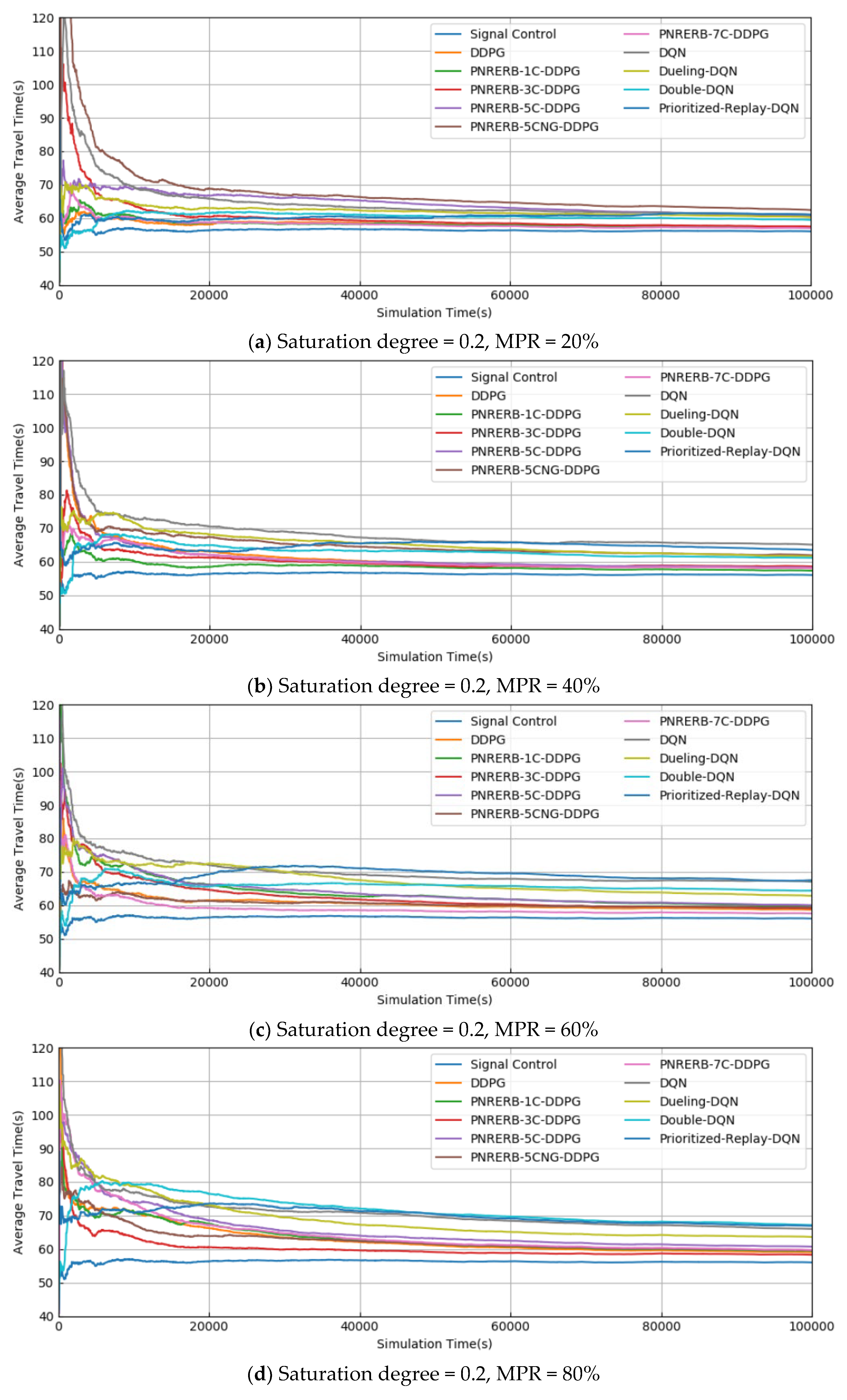
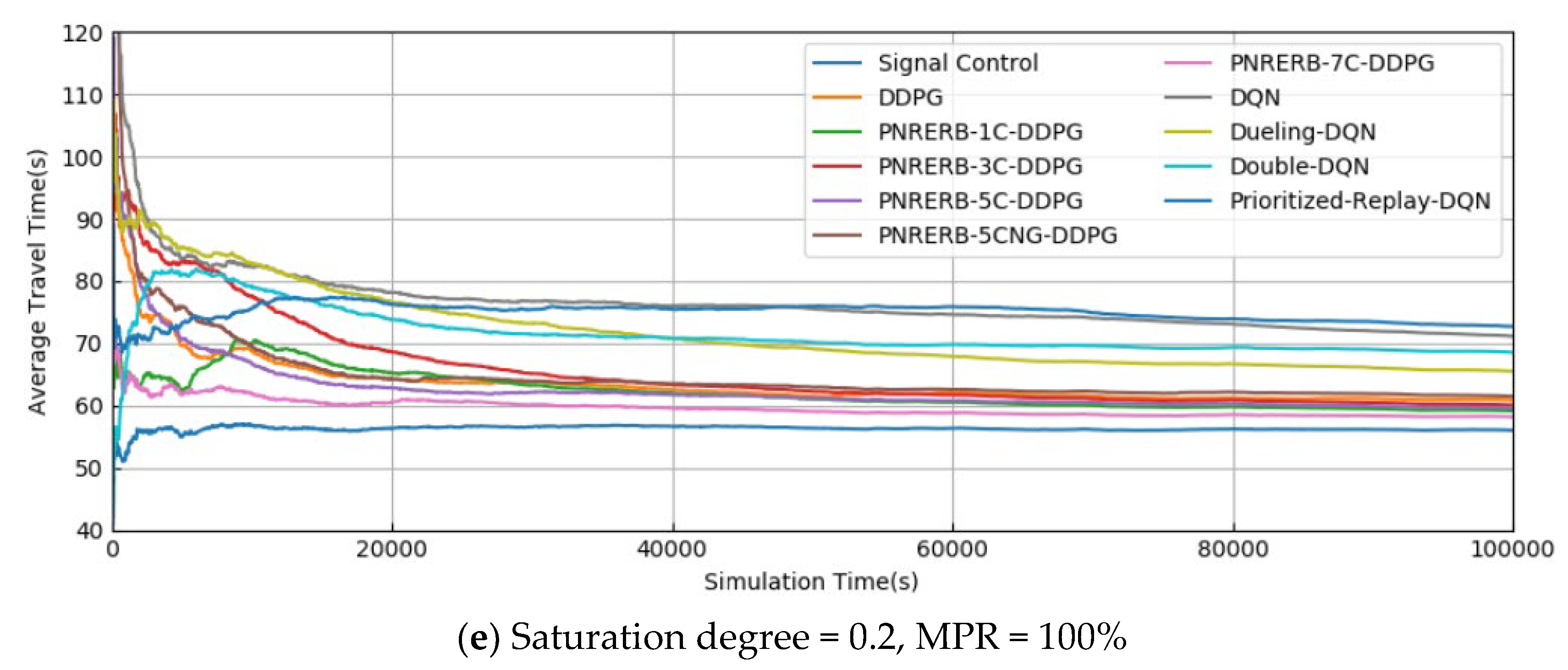
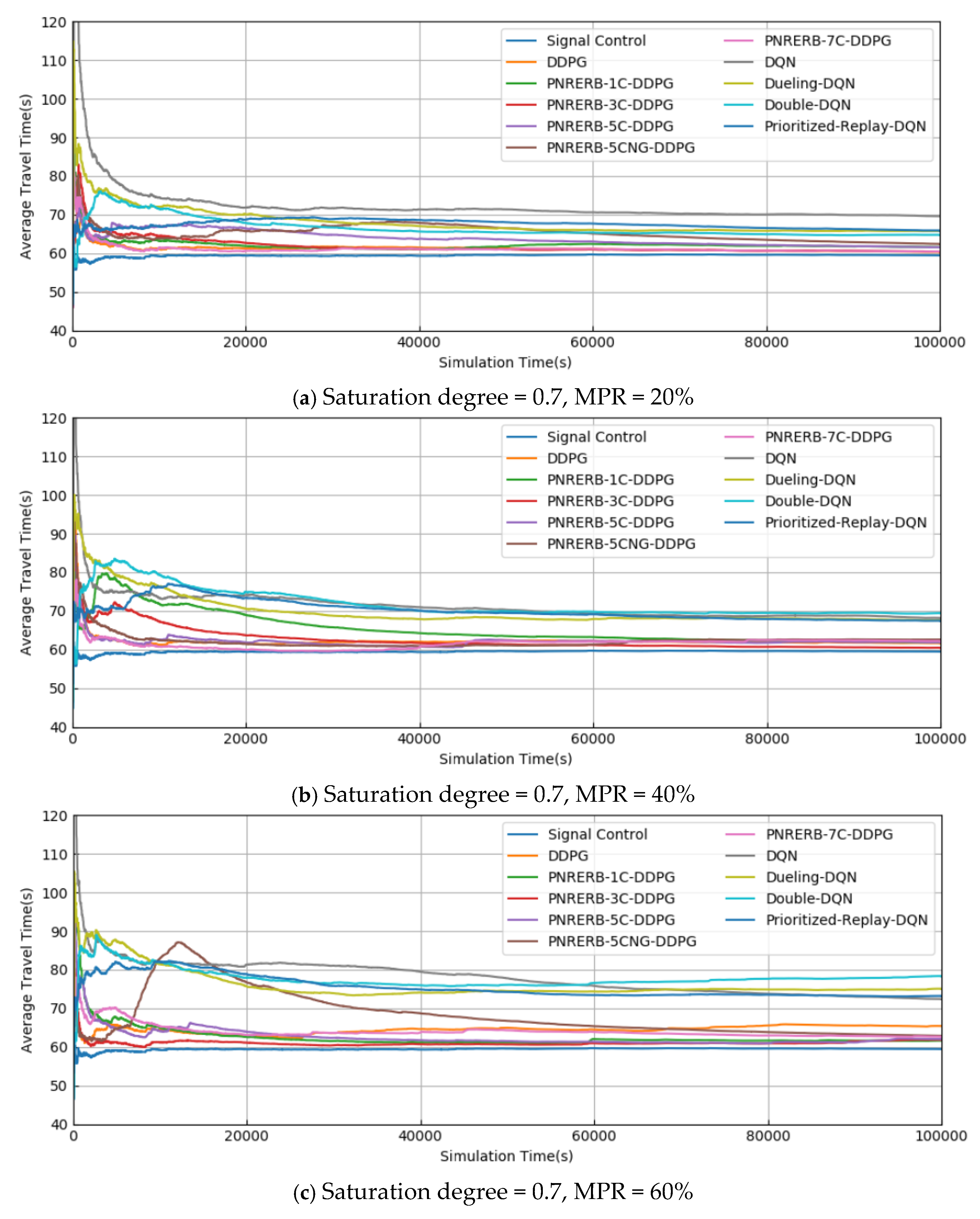
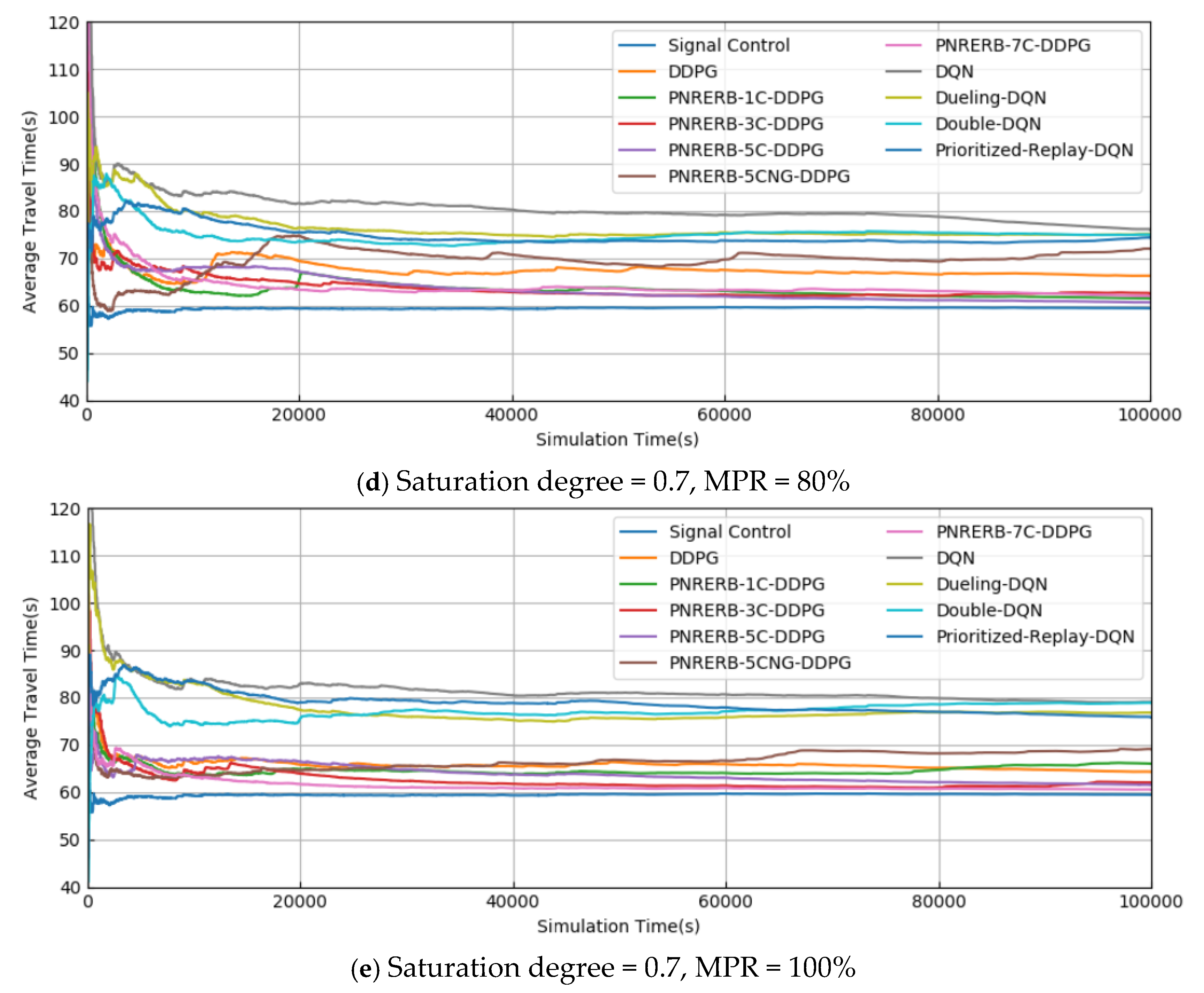
5.1. Training Results

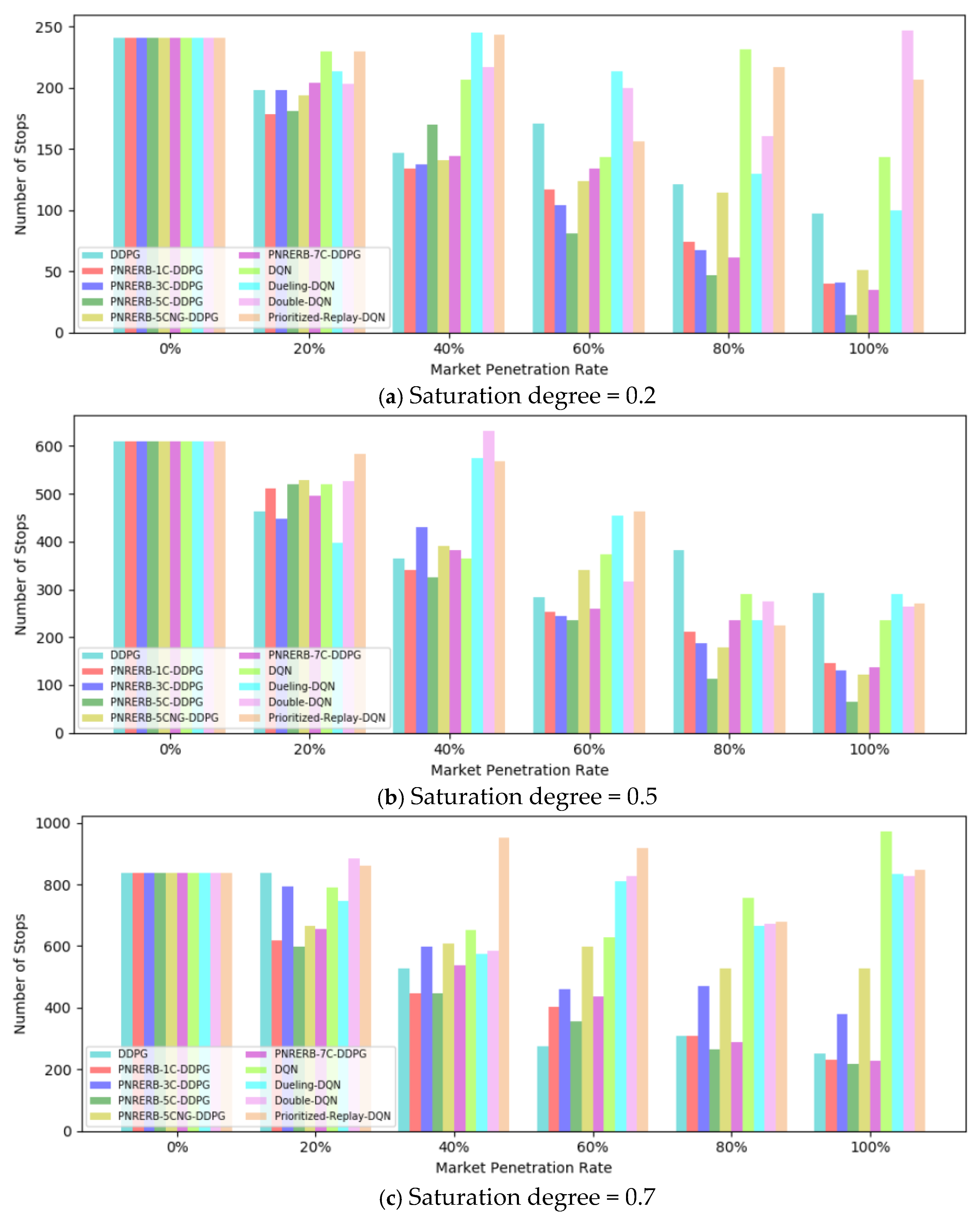
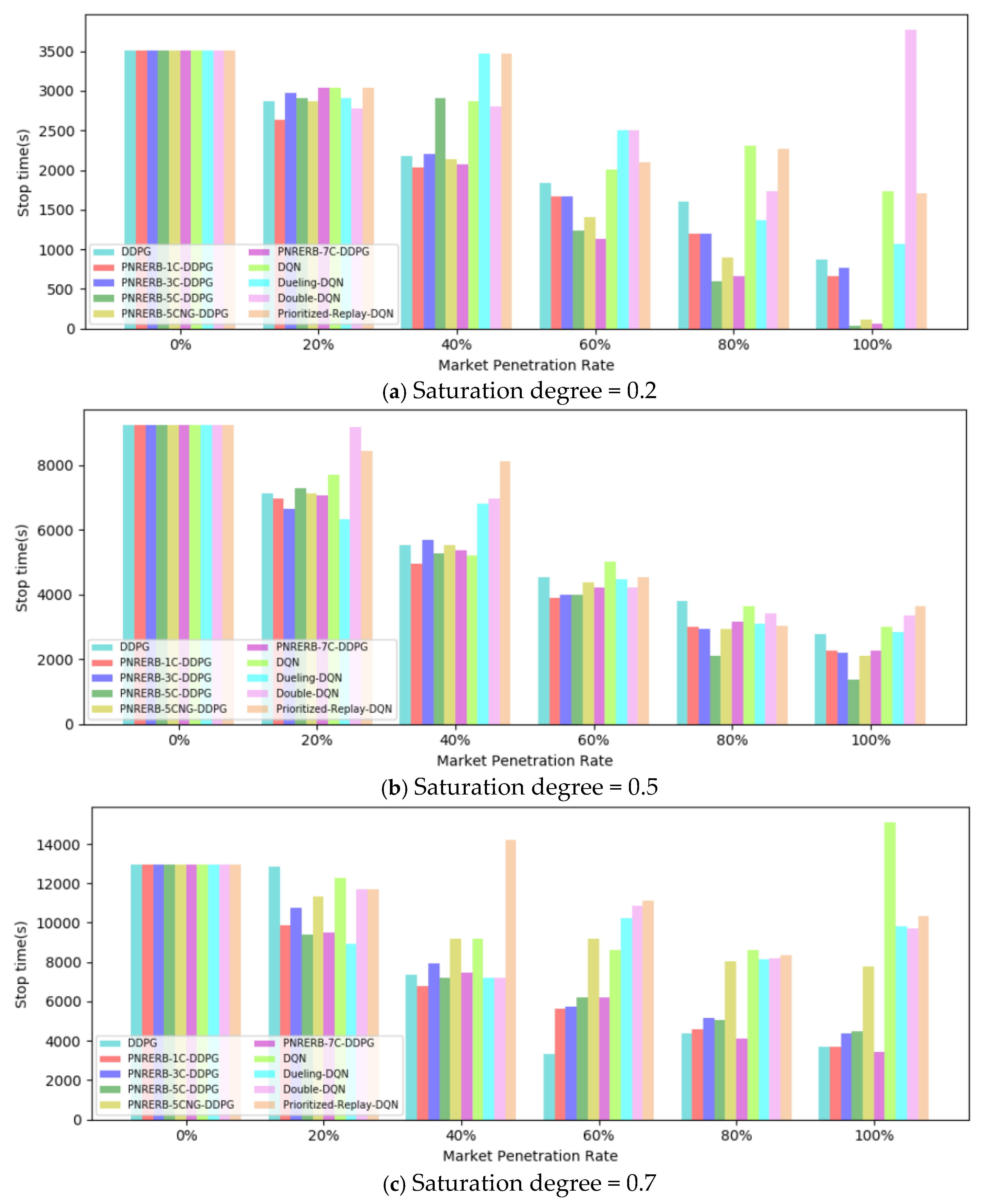
In order to verify the effectiveness of the methods in this paper, 10 methods are trained, respectively. The 10 RL methods are verified under the saturation degrees of 0.2, 0.5, and 0.7, the market penetration rate (MPR) of the CAV market is divided into six types: 0%, 20%, 40%, 60%, 80%, and 100%. Therefore, the training experiment consists of 153 experiments (including three signal control experiments, 90 DDPG-based experiments, and 60 DQN-based experiments. The signal control experiments refer to the situation in which the MPR of the CAV market is 0%.). Each experiment is repeated five times, and the result is the average of five times. The VISSIM simulation random seed is set as 41.

In this paper, the average travel time (ATT) [28] is taken as the evaluation index of training convergence. The calculating equation of ATT is described as shown in Equation (16). At 100,000 simulation seconds, 153 groups of experiments all converged. So, the experiment in each group is trained for 100,000 s. The training results of 100,000 s are analyzed, and the model trained under 100,000 s is used as an evaluation model for subsequent test verification.

$$k_{ATT}=\frac{1}{n}{\displaystyle {\sum }_{k=0}^{n}T{T}_k}$$

(16)

Equation (16) represents the ATT of all the vehicles, from entering the control area to leaving the control area of the intersection. Here, $k_{ATT}$ represents ATT, $T{T}_k$ represents the travel time of the $k$th vehicle, and $n$ represents the number of vehicles leaving the control area of the intersection within the total simulation time.

Figure 4 shows the ATT results under different CAV MPR for 10 methods under the saturation of 0.2.

Table 2. ATT results of different saturation.

Saturation Degree = 0.2
	Benchmark	DDPG-Based Methods						DQN-Based Methods
MPR	M0	M1	M2	M3	M4	M5	M6	M7	M8	M9	M10
0%	56.0	56.0	56.0	56.0	56.0	56.0	56.0	56.0	56.0	56.0	56.0
20%	/	57.3	57.3	57.4	60.5	62.4	56.9	61.0	60.2	59.4	61.0
40%	/	58.0	57.3	58.5	58.2	61.9	58.0	65.0	61.5	61.1	63.4
60%	/	58.6	59.7	59.0	60.0	59.3	57.5	67.0	62.8	64.3	67.5
80%	/	59.0	59.4	58.3	60.7	59.6	59.7	66.0	63.6	67.1	66.9
100%	/	60.9	59.1	60.0	59.5	61.4	58.2	71.1	65.5	68.5	72.7
Saturation Degree = 0.5
	Benchmark	DDPG-Based Methods						DQN-Based Methods
MPR	M0	M1	M2	M3	M4	M5	M6	M7	M8	M9	M10
0%	57.6	57.6	57.6	57.6	57.6	57.6	57.6	57.6	57.6	57.6	57.6
20%	/	58.7	59.9	58.8	58.7	61.2	58.7	63.3	63.2	62.7	62.8
40%	/	61.1	58.5	58.8	57.9	61.9	58.9	64.4	63.5	67.8	65.2
60%	/	60.2	59.4	59.2	59.1	64.2	60.7	70.6	66.7	70.0	74.5
80%	/	60.9	60.6	60.3	59.9	68.4	59.6	75.3	68.3	72.0	64.6
100%	/	66.6	62.2	62.8	58.8	69.8	61.5	75.3	73.1	74.2	67.6
Saturation Degree = 0.7
	Benchmark	DDPG-Based Methods						DQN-Based Methods
MPR	M0	M1	M2	M3	M4	M5	M6	M7	M8	M9	M10
0%	59.4	59.4	59.4	59.4	59.4	59.4	59.4	59.4	59.4	59.4	59.4
20%	/	60.3	61.5	60.4	61.5	62.4	60.4	69.5	65.7	64.7	65.8
40%	/	62.1	62.3	60.9	62.3	62.5	62.6	73.1	70.5	72.4	69.4
60%	/	65.3	61.6	61.8	62.0	62.8	62.6	72.4	75.0	78.3	73.2
80%	/	66.3	61.5	62.6	60.6	72.0	62.0	76.1	75.1	75.0	74.4
100%	/	64.7	66.5	62.5	62.0	69.1	61.0	78.0	76.7	76.8	75.8

M0: Signal control method; M1: DDPG method; M2: PNRERB-1C-DDPG method; M3: PNRERB-3C-DDPG method; M4: PNRERB-5C-DDPG method; M5: PNRERB-5CNG-DDPG method; M6: PNRERB-7C-DDPG method; M7: DQN method; M8: Dueling DQN method; M9: Double-DQN method; M10: Prioritized Replay DQN method.

shows ATT values after they have converged. Benchmark means the signal control method. According to Figure 4, the ATT of 10 methods all converge, but four methods (DQN, Dueling DQN, Double DQN, and Prioritized Replay DQN) get larger ATT values than the other six methods. As the MPR is 0%, all vehicles are HVs. HVs drive at the maximum desired speed. Therefore, as can be seen in Figure 4, the ATT is the shortest in the cases of 0%. In addition, under either method, the ATT curve rises first and then converges to a smaller value. This is because at the beginning of training, in order to enable the agent to explore more excellent policies, we set a random exploration noise value.

As we can see from Figure 4 and Table 2, on the whole, DDPG-based methods are better than DQN-based methods. Most DDPG-based methods can get a smaller ATT (less than 60 s), but for some methods (such as the PNRERB-5CNG-DDPG method, which is caused by the absence of the preceding vehicle state handling method in the input of the model), they get a slightly larger value. Besides, most DQN-based methods can get larger ATT values (more than 60 s).

Figure 5 shows the convergence of ATT values for different CAV MPRs for 10 methods under the saturation of 0.5. As can be seen from Figure 5 and Table 2, except for the ATT obtained by DQN, Dueling DQN, Double DQN, Prioritized Replay DQNP, NRERB-3C-DDPG, and PNRERB-5CNG-DDPG being relatively large, the ATT values obtained by the 10 methods eventually can get a stable value. Compared with Figure 5c–e, the ATT values obtained by Figure 5a,b are larger and less stable, especially for DQN-based methods. In addition, the stable ATT values of the PNRERB-5CNG-DDPG method are all larger than those of the DDPG method. When the MPR is 100%, most methods all get a higher ATT value, which means that with a low MPR, we can get a better value than that with a higher MPR.

Figure 6 shows the convergence of ATT values for different CAV MPRs for 10 methods under the saturation degree of 0.7. As can be seen from Figure 6 and Table 2, the ATT for 10 methods eventually tends to be stable. However, compared with Figure 4 and Figure 5, the values of the 10 methods in Figure 6 are relatively larger. Likewise, the DQN-based method and PNRERB-5CNG-DDPG method have certain fluctuation, while the volatility of the other five methods is small. This is because DQN-based methods discretize the action, which results in worse strategies. The PNRERB-5CNG-DDPG method does not adopt the state processing method of the preceding vehicle, resulting in inaccurate judgment of the state of the preceding vehicle, and a long ATT. Among the PNRERB-1C-DDPG, PNRERB-3C-DDPG, PNRERB-5C-DDPG, and PNRERB-7C-DDPG methods, the ATT obtained by the PNRERB-7C-DDPG method is the most stable.

In conclusion, Figure 4, Figure 5 and Figure 6 show that the ATT in each case converges under the three saturation conditions. However, compared with the method that does not adopt the preceding vehicle state processing method (PNRERB-5CNG-DDPG), the method that adopts the preceding vehicle state processing method has a better effect (PNRERB-5C-DDPG). In addition, DQN-based methods can learn worse strategies than the DDPG-based method, resulting in larger ATT values. Finally, compared with Figure 4, Figure 5 and Figure 6, there is a certain difference in the convergence of the ATT curve, which also reflects the randomness of the DRL method, so repeated experiments are needed.

5.2. Test Results

After the training period, the trained models are applied to test the efficiency of the RL algorithm. In order to eliminate the contingency of the algorithm, this paper carries out simulation under the random seeds 38, 40, 42, 44, and 46 of VISSIM. Each simulation time is 10,800 s (3 h). Finally, the mean value of five group experiments for each method was taken as the final analysis result.

In order to verify the validity of the algorithm in this paper, the same as the training, 10 methods under the saturation of 0.2, 0.5, and 0.7 were tested. The number of stops, stop time, delay, and fuel consumption and exhaust emission are used as evaluation index. The benefits are calculated by Equations (17)–(19):

$$B_{number-of-stops}=\frac{N{S}_{RL}-N{S}_s}{N{S}_s}\times 100\%$$

(17)

$$B_{stop-time}=\frac{S{T}_{RL}-S{T}_s}{S{T}_s}\times 100\%$$

(18)

$$B_{delay}=\frac{D_{RL}-D_s}{D_s}\times 100\%$$

(19)

Here, $B_{number-of-stops}$, $B_{stop-time}$, and $B_{delay}$ represent the number of stops, stop time, and delay benefits respectively, $N{S}_{RL}$, $S{T}_{RL}$ and $D_{RL}$ are the number of stops, stop time, and delay obtained from the RL algorithm. $N{S}_s$, $S{T}_s$, and $D_s$ are the number of stops, stop time, and delay obtained from the signal control method.

Figure 7 is a comparison diagram of the number of stops for the 10 methods under the saturation degrees of 0.2, 0.5, and 0.7, respectively.

Table 3. Benefits of the number of stops.

Saturation Degree = 0.2 (%)
	DDPG-Based Methods						DQN-Based Methods
MPR	M1	M2	M3	M4	M5	M6	M7	M8	M9	M10
20%	17	26	17	24	19	15	4	11	15	4
40%	39	44	43	29	41	40	14	−1	10	−1
60%	29	51	56	66	48	44	40	11	17	35
80%	49	69	72	80	52	74	4	46	33	10
100%	59	83	82	94	78	85	40	58	−2	14
Saturation Degree = 0.5 (%)
	DDPG-Based Methods						DQN-Based Methods
MPR	M1	M2	M3	M4	M5	M6	M7	M8	M9	M10
20%	23	16	26	14	13	18	14	34	13	4
40%	40	44	29	46	35	37	40	5	−3	6
60%	53	58	59	61	44	57	38	25	48	24
80%	37	65	69	81	70	61	52	61	54	63
100%	52	76	78	89	79	77	61	52	56	55
Saturation Degree = 0.7 (%)
	DDPG-Based Methods						DQN-Based Methods
MPR	M1	M2	M3	M4	M5	M6	M7	M8	M9	M10
20%	0	26	5	28	20	21	5	11	−5	−2
40%	36	46	28	46	27	35	22	31	30	−13
60%	67	52	45	57	28	47	24	3	1	−9
80%	63	63	43	68	36	65	9	20	19	18
100%	69	72	54	73	36	72	−16	0	1	−1

M1: DDPG method; M2: PNRERB-1C-DDPG method; M3: PNRERB-3C-DDPG method; M4: PNRERB-5C-DDPG method; M5: PNRERB-5CNG-DDPG method; M6: PNRERB-7C-DDPG method; M7: DQN method; M8: Dueling-DQN method; M9: Double-DQN method; M10: Prioritized-Replay-DQN method; MPR: market penetration rate.

shows the benefits of the number of stops for 10 methods under three saturation degrees. The 0% MPR means that all vehicles are HVs, having the same meaning as shown in Figure 8 and Figure 9. As can be seen from the (a), (b), and (c) graphs in Figure 7 and Table 3, the 10 methods can reduce the number of stops. The highest benefits of the saturation degrees of 0.2, 0.5, and 0.7 are 94%, 89%, and 73%, respectively.

As can be seen from the (a), (b), and (c) graphs in Figure 7, as the MPR of the CAVs increases, the number of stops gradually decreases for the DDPG-based methods. However, the DQN-based methods all get a worse result than the DDPG-based method. At penetration rates of 20% and 40%, the benefits of the six DDPG methods differ little. However, when the penetration rate is 60%, 80%, or 100%, the benefits gap is relatively obvious. Among the six methods, the DDPG method with multi-critics is better than the traditional DDPG method, while among the DDPG methods with multi-critics, the PNRERB-5CNG-DDPG method has the lowest benefits. This is because PNRERB-5CNG-DDPG does not consider the preceding vehicle state processing method, and the CAV is influenced by the HV. The benefit difference between PNRERB-1C-DDPG, PNRERB-3C-DDPG and PNRERB-7C-DDPG is not obvious. Relatively, the benefit of the PNRERB-5C-DDPG method is the highest, the total number of stops in 3 h is reduced to 14, and the benefit is up to 94%.

Similarly, it can be seen from Table 3 that the benefits of the number of stops under the saturation degrees of 0.2, 0.5, and 0.7 are different. However, in general, the benefits under 0.2 and 0.5 saturation degrees are higher than that for 0.7. Moreover, with a higher MPR, most methods can get higher benefits. However, some DQN-based methods (such as the Prioritized Replay DQN method) can get a minus result, which means that the number of stops optimized by this DQN’s method is higher than that of the signal control.

Figure 8 is comparison diagram of the stop times of different CAV MPRs for 10 methods under the saturation degrees of 0.2, 0.5 and 0.7.

Table 4. Benefits of stop time.

Saturation Degree = 0.2 (%)
	DDPG-Based Methods						DQN-Based Methods
MPR	M1	M2	M3	M4	M5	M6	M7	M8	M9	M10
20%	18	24	15	17	18	13	13	17	20	13
40%	38	41	37	17	39	40	18	1	20	1
60%	47	52	52	64	59	67	42	28	28	40
80%	54	65	65	82	74	80	34	60	50	35
100%	75	80	78	99	96	98	50	69	−7	51
Saturation Degree = 0.5 (%)
	DDPG-Based Methods						DQN-Based Methods
MPR	M1	M2	M3	M4	M5	M6	M7	M8	M9	M10
20%	22	24	28	21	22	23	16	31	1	8
40%	40	46	38	42	40	42	43	26	24	12
60%	50	57	57	57	52	54	45	51	54	50
80%	58	67	68	77	68	65	60	66	62	67
100%	70	75	76	85	77	75	67	69	63	60
Saturation Degree = 0.7 (%)
	DDPG-Based Methods						DQN-Based Methods
MPR	M1	M2	M3	M4	M5	M6	M7	M8	M9	M10
20%	1	23	16	27	12	26	5	30	9	9
40%	43	47	38	44	29	42	29	44	44	−9
60%	74	56	55	52	29	52	33	20	16	14
80%	66	64	60	61	38	68	33	37	36	35
100%	71	71	66	65	39	73	−16	24	24	20

M1: DDPG method; M2: PNRERB-1C-DDPG method; M3: PNRERB-3C-DDPG method; M4: PNRERB-5C-DDPG method; M5: PNRERB-5CNG-DDPG method; M6: PNRERB-7C-DDPG method; M7: DQN method; M8: Dueling-DQN method; M9: Double-DQN method; M10: Prioritized-Replay-DQN method; MPR: market penetration rate.

shows the benefits of the stop time for 10 methods under three different saturation degrees. It can be seen from (a), (b), and (c) in Figure 8 and Table 4 that the stop time of each vehicle is reduced for a certain extent of 10 RL-based methods under the saturation degrees of 0.2, 0.5, and 0.7. The maximum benefits of saturation of 0.2, 0.5, and 0.7 are 99%, 85%, and 73% respectively.

Figure 8a–c show that under three different saturation degrees, with the increasing MPR, the stop time decreases gradually and the benefits increase gradually, except for some DQN-based methods (such as the Double-DQN method under 0.2 saturation). When the MPR is 60%, 80%, and 100% under the 0.2 saturation degree, the three methods of PNRERB-5C-DDPG, PNRERB-5CNG-DDPG and PNRERB-7C-DDPG are better than DDPG, PNRERB-1C-DDPG, and PNRERB-3C-DDPG, with the highest benefits of 99%, 97%, and 98%, respectively. For the five MPRs, the stop time of PNRERB-1C-DDPG, PNRERB-3C-DDPG, PNRERB-5CNG-DDPG, and PNRERB-7C-DDPG has little difference under 0.5 saturation. However, the stop time benefit of the DDPG method is slightly less.

For Figure 8 and Table 4, under the saturation degree of 0.7, the benefits of the PNRERB-5CNG-DDPG method are the lowest for the DDPG-based methods. When the MPR is 20% and 40%, the benefits of PNRERB-1C-DDPG, PNRERB-5C-DDPG, and PNRERB-7C-DDPG methods are higher. However, when the MPR is 60%, the DDPG method has the highest profit, reaching 74%. When the MPR is 80% and 100%, DDPG, PNRERB-1C-DDPG, and PNRERB-7C-DDPG reduce the stop time the most, while PNRERB-3C-DDPG and PNRERB-5C-DDPG reduce the stop time the second most. In addition, the benefit obtained by the DDPG method includes the lowest benefit of 1% and the highest benefit of 74%, which also reflects the instability of the original DDPG method. DQN-based methods get a lower benefit relatively, while some methods get a negative benefit (such as the Prioritized-Replay-DQN method).

Figure 9 is a comparison diagram of the delay of different CAV MPRs under the saturation degrees of 0.2, 0.5, and 0.7 for 10 methods.

Table 5. Benefits of delay.

Saturation Degree = 0.2 (%)
	DDPG-Based Methods						DQN-Based Methods
MPR	M1	M2	M3	M4	M5	M6	M7	M8	M9	M10
20%	12	16	11	12	8	12	6	7	11	−3
40%	26	31	28	18	13	33	12	−2	8	−1
60%	41	41	41	51	31	41	25	20	16	18
80%	43	61	57	73	50	63	18	33	36	18
100%	64	72	69	93	64	67	26	51	−2	33
Saturation Degree = 0.5 (%)
	DDPG-Based Methods						DQN-Based Methods
MPR	M1	M2	M3	M4	M5	M6	M7	M8	M9	M10
20%	12	6	12	11	10	9	1	−4	−21	−1
40%	20	24	16	22	20	19	−31	5	−25	5
60%	28	31	33	33	31	28	−13	22	27	15
80%	30	51	42	43	36	45	23	30	24	30
100%	37	63	51	55	46	43	27	32	22	19
Saturation Degree = 0.7 (%)
	DDPG-Based Methods						DQN-Based Methods
MPR	M1	M2	M3	M4	M5	M6	M7	M8	M9	M10
20%	1	9	5	9	−17	10	−54	−29	−14	−5
40%	20	23	16	17	5	20	−3	2	1	−39
60%	35	29	25	26	6	27	−29	3	−0	−13
80%	38	42	31	34	11	30	−60	−8	−8	−16
100%	44	52	37	41	16	37	−45	−8	−7	−9

M1: DDPG method; M2: PNRERB-1C-DDPG method; M3: PNRERB-3C-DDPG method; M4: PNRERB-5C-DDPG method; M5: PNRERB-5CNG-DDPG method; M6: PNRERB-7C-DDPG method; M7: DQN method; M8: Dueling-DQN method; M9: Double-DQN method; M10: Prioritized-Replay-DQN method; MPR: market penetration rate.

shows benefits of stop time for 10 methods under three different saturation degrees. As can be seen from Figure 9, under the saturation degrees of 0.2, 0.5, and 0.7, the delay of vehicles is reduced to a certain extent and obtains the great benefits of the 10 RL-based methods, except for some of the DQN-based methods (such as the Double-DQN method and Prioritized-Replay-DQN method). In addition, the overall benefits at a saturation degree of 0.2 are greater than those of the saturation degrees 0.5 and 0.7. At the same time, in the case of a low MPR, except for the PNRERB-5CNG-DDPG method with the saturation degree of 0.7, the difference of benefits obtained by the other five DDPG-based methods is not obvious.

For Figure 9 and Table 5, the delays and benefits are worse for the DQN-based methods compared with the DDPG-based methods, in which the DQN-based methods can get large negative benefits. However, for the 0.2 and 0.5 saturation degrees, the DQN-based methods can get some benefits. For the DDPG-based methods, under the saturation degree of 0.2, the PNRERB-5CNG-DDPG method obtained the lowest benefit, while the PNRERB-5C-DDPG method obtained the highest, up to 93% under a MPR of 100%. When the saturation is 0.5 and MPR is 60% or above, the benefits obtained by the methods of PNRERB-1C-DDPG, PNRERB-3C-DDPG, and PNRERB-5C-DDPG are higher. Especially when the MPR is 100%, the benefits are all above 50%, while that for the DDPG is the least: only 37%. Under the saturation degree of 0.7, the optimization of the PNRERB-5CNG-DDPG method obtained the highest delay and the lowest benefits. Especially when the MPR is 20%, the benefits are −17%, which increased the vehicle delay.

Table 6. Total fuel consumption (TFC) and total exhaust emission (TEE) values under saturation degrees of 0.2/0.5/0.7.

	Methods	MPR	Saturation Degree = 0.2		Saturation Degree = 0.5		Saturation Degree = 0.7
			TFC (L)	TEE (kg)	TFC (L)	TEE (kg)	TFC (L)	TEE (kg)
Benchmark	M0	0%	13.66	31.57	34.38	79.54	49.18	113.80
DDPG-based methods	M1	20%	13.77	31.83	34.87	80.69	49.22	113.89
	M2		13.67	31.60	34.40	79.59	49.39	114.29
	M3		13.71	31.70	34.29	79.32	49.14	113.71
	M4		13.82	31.94	34.36	79.49	49.39	114.31
	M5		14.02	32.43	34.37	79.51	52.56	121.65
	M6		13.65	31.54	34.50	79.82	49.00	113.39
DQN-based methods	M7		14.17	32.79	35.97	83.31	59.82	138.72
	M8		14.18	32.82	37.07	85.92	56.62	131.21
	M9		13.99	32.37	38.12	88.28	53.64	124.24
	M10		14.91	34.52	35.89	83.12	52.45	121.54
DDPG-based methods	M1	40%	13.66	31.57	34.48	79.79	49.38	114.30
	M2		13.63	31.51	34.38	79.53	48.96	113.28
	M3		14.44	33.39	34.40	79.59	48.89	113.15
	M4		13.63	31.54	34.40	79.59	49.94	115.59
	M5		14.46	33.43	34.43	79.67	50.27	116.35
	M6		13.63	31.52	34.56	79.97	49.17	113.80
DQN-based methods	M7		14.56	33.74	43.36	100.68	54.38	126.15
	M8		14.50	33.62	36.69	84.99	53.57	124.12
	M9		14.77	34.18	39.93	92.46	53.62	124.27
	M10		14.52	33.62	35.73	82.75	61.12	141.98
DDPG-based methods	M1	60%	13.76	31.81	34.27	79.29	50.53	116.97
	M2		13.62	31.48	34.38	79.53	49.36	114.24
	M3		13.63	31.52	35.23	81.53	48.75	112.82
	M4		13.68	31.63	34.86	80.68	50.00	115.72
	M5		14.06	32.50	35.00	80.98	50.44	116.73
	M6		13.68	31.64	35.16	81.36	49.31	114.11
DQN-based methods	M7		15.31	35.48	41.05	95.27	59.98	139.14
	M8		14.15	32.76	36.31	84.16	52.12	128.73
	M9		14.79	34.26	36.61	84.86	53.34	128.99
	M10		15.81	36.72	37.23	85.02	58.53	135.74
DDPG-based methods	M1	80%	13.65	31.55	34.23	79.20	49.41	114.37
	M2		13.91	32.16	34.43	79.66	48.91	113.17
	M3		13.76	31.81	34.27	79.27	48.87	113.07
	M4		13.71	31.70	35.38	81.85	50.70	114.73
	M5		14.02	32.41	37.87	87.83	50.32	116.43
	M6		13.98	32.32	35.75	82.78	49.09	113.59
DQN-based methods	M7		15.11	34.86	37.52	87.10	64.33	149.35
	M8		16.00	37.07	37.45	86.84	52.34	123.54
	M9		14.60	33.81	37.34	87.02	52.69	124.63
	M10		14.98	34.73	37.41	86.72	55.64	132.56
DDPG-based methods	M1	100%	13.69	31.656	34. 45	79.70	49.64	114.91
	M2		13.71	31.697	34. 26	79.26	49.09	113.58
	M3		13.71	31.707	34.16	79.02	49.08	113.57
	M4		14.17	32.783	35.58	82.30	51.29	118.69
	M5		14.21	32.855	38.38	89.04	50.03	115.76
	M6		13.76	31.816	35.25	81.53	49.12	113.64
DQN-based methods	M7		17.83	41.360	38.08	88.43	69.53	161.24
	M8		14.43	33.426	41.78	96.78	58.12	132.94
	M9		14.48	33.511	39.72	89.75	58.02	132.85
	M10		17.67	40.984	40.01	90.15	58.32	135.21

M0: Signal control method; M1: DDPG method; M2: PNRERB-1C-DDPG method; M3: PNRERB-3C-DDPG method; M4: PNRERB-5C-DDPG method; M5: PNRERB-5CNG-DDPG method; M6: PNRERB-7C-DDPG method; M7: DQN method; M8: Dueling-DQN method; M9: Double-DQN method; M10: Prioritized-Replay-DQN method.

shows the total fuel consumption (TFC) and total exhaust emission (TEE) values of the simulation test for 3 h of the seven methods at saturation degrees of 0.2, 0.5, and 0.7. As can be seen from Table 6, compared with the signal control method, DDPG-based methods have certain changes in TFC and TEE. However, the TFC and TEE values are not increased or decreased significantly relative to the delay and number of stops. For the multi-critic DDPG methods, the DDPG method with fewer critics can generally get fewer TFC and TEE values. This is because the delay and stops can be optimized for DDPG with a large number of critics, with a certain increase in TFC and TEE, while the delay and stops can be optimized for the DDPG method with a small number of critics, as well as TFC and TEE. For DQN-based methods, the TFC and TEE values are larger than those of the DDPG-based methods, which means that the DQN-based methods can get a worse result than the DDPG-based methods.

To sum up, Figure 7, Figure 8 and Figure 9 and Table 3, Table 4 and Table 5 show that the 10 RL-based methods used in this paper have reduced the number of stops, stop times, and delays. Compared with the DDPG-based methods, the DQN-based methods can get a worse result. However, for the DDPG-based methods, the one with the worst optimization result is PNRERB-5CNG-DDPG. The other five DDPG-based methods can get a certain optimization result. Moreover, the DDPG-based methods with fewer critics can get fewer stops, stop times, and delays, simultaneously.

Through the above analysis, we have obtained the optimization results of six DRL methods. In order to further show the driving trajectory of vehicles, this paper chooses the spatial–temporal trajectory of the PNRERB-5C-DDPG method for further analysis, which has better optimization results. Figure 10 is the spatial–temporal trajectory of the PNRERB-5C-DDPG method under different MPRs of a CAV at the saturation degrees of 0.2 and 0.5. Figure 11 shows the spatial–temporal trajectory of the PNRERB-5C-DDPG algorithm under different MPRs of a CAV under the saturation degree of 0.7. The red line represents the trajectory of CAVs, and the blue line represents the trajectory of HVs.

As can be seen from Figure 10, no matter whether at the saturation degree of 0.2 or 0.5, as the MPRs of a CAV increases, the stop time of the vehicle gradually decreases, and the trajectory of the vehicle gradually becomes smooth. As for the vehicles entering the control area, this paper adopts the method of random probability to determine whether they are CAVs or not. Therefore, in the spatial–temporal trajectory graphs in Figure 10 and Figure 11, it appears that some vehicles are set as CAVs when the MPR is 20%. However, they are not set as CAVs when the MPR is 40% or above. In addition, the random probability method is used to determine whether the vehicle is a CAV, which further improves the robustness of the method in this paper. It also avoids only training a CAV in some certain situations, which is more consistent with actual situations. Similarly, in Figure 11, the vehicle’s trajectory becomes smoother as the MPR of the CAV increases. However, compared with Figure 10, the trajectory optimization of CAVs under the saturation degree of 0.7 is not good enough. The main reason is that there are more vehicles on the road and the training is not perfect due to the influence of the stability of the DRL method. Figure 11f shows that even when the MPR of a CAV is 100%, a large number of vehicles still stop.

In a word, when the saturation degree is small (0.2 and 0.5), the spatial–temporal trajectory optimization of the vehicle is better, the vehicle stop time is greatly reduced, and the trajectory is smoother. However, when the saturation is relatively larger, there is still some room for improvement in the spatial–temporal optimization trajectory of the vehicle.

6. Conclusions and Prospect

In view of the mixed driving situation of left-turning CAVs and HVs at a signalized intersection, a DRL model is established. Based on the DRL model, a DDPG method based on positive and negative reward experience replay buffer and multi-critics is designed. In order to verify the effectiveness of 10 methods, this paper verified the optimization effects of DDPG, PNRERB-1C-DDPG, PNRERB-3C-DDPG, PNRERB-5C-DDPG, PNRERB-5CNG-DDPG, PNRERB-7C-DDPG, DQN, Dueling DQN, Double DQN, and Prioritized Replay DQN under saturation degrees of 0.2, 0.5, and 0.7, respectively.

In general, compared with the traditional signal control method, the number of stops, stop times, and vehicle delays are all reduced to some extent for the 10 RL-based methods. Under the saturation degrees of 0.2 and 0.5, the optimization results of PNRERB-1C-DDPG, PNRERB-3C-DDPG, PNRERB-5C-DDPG, and PNRERB-7C-DDPG among the 10 methods were the best, while the optimization results of DDPG and PNRERB-5CNG-DDPG were worse, and the DQN-based methods were worst. At the saturation degree of 0.7, the optimization result of the PNRERB-5CNG-DDPG method for the DDPG-based method was the worst, and the other five DDPG-based methods were better. In addition, when the MPR is small, the optimization results of the six DDPG-based methods are not much different. When the permeability is large, the optimization results of the six DDPG-based methods are obviously different. Optimizing the number of stops, stop times, and vehicle delays has also led to increased fuel consumption and exhaust emissions (DQN-based methods are the highest). In a word, the introduction of CAVs into traditional vehicles can reduce the delay of vehicles to a certain extent, and the delay size varies with the saturation and MPR.

When designing the reward function of DRL, this paper gives a relatively large punishment for vehicle stops. Therefore, during the learning process, the agent takes a stop as the primary optimization objective, resulting in a certain increase in fuel consumption and exhaust emission. In addition, this paper only considers the application of the DRL method to single signalized intersections, and it can also apply the DRL method to more complex signalized intersections.

References

1. Zhang, M.; Wang, Y.; Zheng, B.; Zhang, K. Application of artificial intelligence in autonomous vehicles. Auto Ind. Res. 2019, 3, 2–7. [Google Scholar]
2. Zhou, B. 2019 autonomous vehicle maturity index report. China Information World, 9 September 2019. [Google Scholar]
3. Xie, X.; Wang, Z. SIV-DSS: Smart In-Vehicle Decision Support System for driving at signalized intersections with V2I communication. Transp. Res. C 2018, 90, 181–197. [Google Scholar] [CrossRef]
4. Vahidi, A.; Sciarretta, A. Energy saving potentials of connected and automated vehicles. Transp. Res. C 2018, 95, 822–843. [Google Scholar] [CrossRef]
5. Hou, X.; Wang, L.; Zhang, Q. Thoughts on the development path of auto insurance in the era of 5G driverless cars. Technol. Econ. Guide 2019, 25, 4–6. [Google Scholar]
6. Zhang, Z.; Li, M.; Lin, X.; Wang, Y.; He, F. Multistep speed prediction on traffic networks: A deep learning approach considering spatio-temporal dependencies. Transp. Res. C 2019, 105, 297–322. [Google Scholar] [CrossRef]
7. Li, Y.; Yang, C.; Hou, Z.; Feng, Y.; Yin, C. Data-driven approximate Q-learning stabilization with optimality error bound analysis. Automatica 2019, 103, 435–442. [Google Scholar] [CrossRef]
8. Zhang, W.; Gai, J.; Zhang, Z.; Tang, L.; Liao, Q.; Ding, Y. Double-DQN based path smoothing and tracking control method for robotic vehicle navigation. Comput. Electron. Agric. 2019, 166, 104985. [Google Scholar] [CrossRef]
9. Aslani, M.; Seipel, S.; Mesgari, M.S.; Wiering, M. Traffic signal optimization through discrete and continuous reinforcement learning with robustness analysis in downtown Tehran. Adv. Eng. Infor. 2018, 38, 639–655. [Google Scholar] [CrossRef]
10. Genders, W.; Razavi, S. Evaluating reinforcement learning state representations for adaptive traffic signal control. Procedia Comput. Sci. 2018, 130, 26–33. [Google Scholar] [CrossRef]
11. Belletti, F.; Haziza, D.; Gomes, G.; Bayen, A.M. Expert Level control of Ramp Metering based on Multi-task Deep Reinforcement Learning. IEEE Trans. Intell. Transp. Syst. 2017, 19, 1198–1207. [Google Scholar] [CrossRef]
12. Wang, P.; Chan, C. Formulation of Deep Reinforcement Learning Architecture Toward Autonomous Driving for On-Ramp Merge. In Proceedings of the IEEE 20th International Conference on ITS, Yokohama, Japan, 16–19 October 2017. [Google Scholar]
13. Sallab, A.E.; Abdou, M.; Perot, E.; Yogamani, S. Deep Reinforcement Learning framework for Autonomous Driving. Electron. Imag. 2017, 19, 70–76. [Google Scholar] [CrossRef] [Green Version]
14. Xu, Y. Research of Traffic Signal Control in Urban Area based on Cooperative Vehicle Infrastructure System. Master’s Thesis, North China University of Technology, Beijing, China, 2017. [Google Scholar]
15. Li, Z.; Elefteriadou, L.; Ranka, S. Signal control optimization for automated vehicles at isolated signalized intersections. Transp. Res. C 2014, 49, 1–18. [Google Scholar] [CrossRef]
16. Sun, X. Estimation of Emission at Signalized Intersection with Vehicle to Infrastructure Communication. Master’s Thesis, Beijing Jiaotong University, Beijing, China, 2016. [Google Scholar]
17. Guo, Y. Research and Implementation of Eco-Driving Guidance System for Intersection. Master’s Thesis, Chang’an University, Xi’an, China, 2017. [Google Scholar]
18. Wang, X. Traffic Signal Coordination Control and Optimization for Urban Arterials Considering the Emission of Platoon. Master’s Thesis, Beijing Jiaotong University, Beijing, China, 2017. [Google Scholar]
19. Li, D. Distinguishing Method of Arterial Fleet Considering Minor Traffic Flow. Master’s Thesis, Jilin University, Changchun, China, 2017. [Google Scholar]
20. Zhou, B. Urban Traffic Signal Control Based on Connected Vehicle Simulation Platform. Master’s Thesis, Zhejiang University, Hangzhou, China, 2016. [Google Scholar]
21. Yu, C.; Feng, Y.; Liu, H.X.; Ma, W.; Yang, X. Integrated optimization of traffic signals and vehicle trajectories at isolated urban intersections. Transp. Res. B 2018, 112, 89–112. [Google Scholar] [CrossRef] [Green Version]
22. Liao, R. Eco-Driving of Vehicle Platoons in Cooperative Vehicle-Infrastructure System at Signalized Intersections. Master’s Thesis, Beijing Jiaotong University, Beijing, China, 2018. [Google Scholar]
23. Zhao, W.M.; Ngoduy, D.; Shepherd, S.; Liu, R.; Papageorgiou, M. A platoon based cooperative eco-driving model for mixed automated and human-driven vehicles at a signalised intersection. Transp. Res. C 2018, 95, 802–821. [Google Scholar] [CrossRef] [Green Version]
24. He, X.; Wu, X. Eco-driving advisory strategies for a platoon of mixed gasoline and electric vehicles in a connected vehicle system. Transp. Res. D 2018, 63, 907–922. [Google Scholar] [CrossRef]
25. Gong, S.; Du, L. Cooperative platoon control for a mixed traffic flow including human drive vehicles and connected and autonomous vehicles. Transp. Res. B 2018, 116, 25–61. [Google Scholar] [CrossRef]
26. Kalantari, R.; Motro, M.; Ghosh, J.; Bhat, C. A distributed, collective intelligence framework for collision-free navigation through busy intersections. In Proceedings of the 2016 IEEE 19th International Conference on Intelligent Transportation Systems (ITSC), Rio de Janeiro, Brazil, 1–4 November 2016; pp. 1378–1383. [Google Scholar]
27. Shi, J.; Qiao, F.; Li, Q.; Yu, L.; Hu, Y. Application and Evaluation of the Reinforcement Learning Approach to Eco-Driving at Intersections under Infrastructure-to-Vehicle Communications. Transp. Res. Rec. 2018, 2672, 89–98. [Google Scholar] [CrossRef]
28. Matsumoto, Y.; Nishio, K. Reinforcement Learning of Driver Receiving Traffic Signal Information for Passing through Signalized Intersection at Arterial Road. Transp. Res. Procedia 2019, 37, 449–456. [Google Scholar] [CrossRef]
29. Lillicrap, T.P.; Hunt, J.J.; Pritzel, A.; Heess, N.; Erez, T.; Tassa, Y.; Silver, D.; Wierstra, D. Continuous control with deep reinforcement learning. Comput. Sci. 2015, 8, A187. [Google Scholar]
30. Silver, D.; Lever, G.; Heess, N.; Degris, T. Deterministic Policy Gradient Algorithms. In Proceedings of the 31st International Conference on Machine Learning (ICML), Beijing, China, 21–26 June 2014. [Google Scholar]
31. Witten, I.H. An adaptive optimal controller for discrete-time Markov environments. Inf. Control 1977, 34, 286–295. [Google Scholar] [CrossRef] [Green Version]
32. Zuo, S.; Wang, Z.; Zhu, X.; Ou, Y. Continuous reinforcement learning from human demonstrations with integrated experience replay for autonomous driving. In Proceedings of the 2017 IEEE International Conference on Robotics and Biomimetics (ROBIO), Macau, 5–8 December 2017; pp. 2450–2455. [Google Scholar]
33. Zhu, M.; Wang, X.; Wang, Y. Human-like autonomous car-following model with deep reinforcement learning. Transp. Res. C 2018, 97, 348–368. [Google Scholar] [CrossRef] [Green Version]
34. Xu, J. Intersection blind spot collision avoidance technology based on Vehicle Infrastructure Cooperative Systems. Master’s Thesis, Tianjin University of Technology and Education, Tianjin, China, 2016. [Google Scholar]
35. Jiang, H. Research on eco-driving control at signalized intersections under connected and automated vehicles environment. Ph.D. Thesis, Harbin Institute of Technology, Harbin, China, 2018. [Google Scholar]
36. Sutton, R.; Barto, A.G. Reinforcement Learning: An Introduction; MIT Press: Cambridge, MA, USA, 1998. [Google Scholar]
37. Wang, X.; He, H.; Xu, X. Reinforcement learning algorithm for partially observable Markov decision processes. Control Decis. 2004, 19, 1263–1266. [Google Scholar]
38. Lin, L.J. Reinforcement Learning for Robots Using Neural Networks; School of Computer Science, Carnegie-Mellon Univ.: Pittsburgh, PA, USA, 1993. [Google Scholar]
39. Wu, J.; Wang, R.; Li, R.; Zhang, H.; Hu, X. Multi-critic DDPG Method and Double Experience Replay. In Proceedings of the 2018 IEEE International Conference on Systems, Man, and Cybernetics (SMC), Miyazaki, Japan, 7–10 October 2018; pp. 165–171. [Google Scholar]
Figure 1. The road network structure.
Information 11 00077 g001
Figure 2. Interaction between the PNRERB-MC-DDPG method and VISSIM software.
Information 11 00077 g002
Figure 3. VISSIM simulation road network.
Information 11 00077 g003
Figure 4. Average travel time (ATT) results for different CAV market penetration rates (MPRs) under 0.2 saturation.
Information 11 00077 g004aInformation 11 00077 g004b
Figure 5. ATT for different CAV penetration rates under saturation degree 0.5.
Information 11 00077 g005aInformation 11 00077 g005b
Figure 6. ATT for different CAV penetration rates under a saturation degree of 0.7.
Information 11 00077 g006aInformation 11 00077 g006b
Figure 7. Comparison diagram of number of stops under different CAV MPRs under saturation degrees of 0.2/0.5/0.7.
Information 11 00077 g007
Figure 8. Comparison diagram of stop times under different CAV MPRs under saturation of 0.2/0.5/0.7.
Information 11 00077 g008
Figure 9. Comparison diagram of delay under different CAV MPRs under saturation degrees of 0.2/0.5/0.7.
Information 11 00077 g009aInformation 11 00077 g009b
Figure 10. Spatial–temporal trajectories for different MPRs under saturation degrees of 0.2 and 0.5.
Information 11 00077 g010aInformation 11 00077 g010bInformation 11 00077 g010cInformation 11 00077 g010d
Figure 11. Spatial–temporal trajectories for different MPRs under the saturation degree of 0.7.
Information 11 00077 g011aInformation 11 00077 g011b