A New Approach to Nonlinear Invariants for Hybrid Systems Based on the Citing Instances Method

Abstract
:1. Introduction
- Guessing a template polynomial of fixed degree as a candidate inductive invariant.
- Defining complete inductive conditions.
- Utilizing a comprehensive Gröbner basis to encode complete inductive conditions into constraints on parameters and, therefore, reducing the invariant generation problem to a non-linear constraint solving problem.
- Solving constraints on parameters. Any solution with respect to the constraints is an inductive invariant.
- Guessing a template polynomial of fixed degree as candidate inductive invariant.
- Defining alternative inductive conditions—which are incomplete but more tractable—to take the place of complete inductive conditions.
- Utilizing a Gröbner basis to encode the alternative inductive conditions into constraints on parameters.
- Solving the constraints. Any solution with respect to the constraints is an inductive invariant.
- Zero Polynomial Theorem [3]: . By the Zero Polynomial Theorem, three constraint equations are obtained synchronously, , solving .
- CIM (this paper): Take four arbitrary distinct values of x and substitute them for x in the left side of (1), respectively. Then, equate the left side of (1) to zero (e.g., when , then is obtained). Hence, four constraint equations can be derived independently: . Solving, we get . Here is an intuitive explanation of CIM: when and the degree of the polynomial in the left side of (1) is 3, the equation must have at most three roots. However, the left side of (1) vanishes over , which means that the equation (1) has at least four roots. Therefore, the equation (1) must be identically equal to zero.
- Guessing a template of a fixed degree as an invariant template.
- Defining the complete inductive conditions.
- Applying a lattice array to the complete inductive conditions to generate the constraint on the parameters.
- Solving the constraint. Any solution to the constraint guarantees the template an inductive invariant.
Related Work
2. Preliminaries
2.1. Basic Lemmas
- 1.
- Determining the size of the lattice array. By observation, the degrees of (3) in x and y are both less than or equal to 2, such that the lattice array size is .
- 2.
- Determining the members of the lattice array. Essentially, the variables can be assigned freely, so we can assign variables which are easy to test. For our convenience, let and . Then, the nine instances in the lattice array are and .
- 3.
- Substituting instances for x and y one by one, test whether the left side of (3) is equal to the right side of (3). If one of them leads to the left side of (3) differing from the right side of (3), it is a counterexample for (3) not being an identity. Otherwise, we can conclude that (3) is an identity.
2.2. Characteristic Set
- 1.
- and s not identically zero;
- 2.
- and , and each is reduced with respect to the preceding polynomials,
2.3. Hybrid System
- L is a finite set of locations (or modes);
- V is a set of real-valued system variables. The hybrid system state space is denoted by , a state is denoted by , and is a continuous state of the variables over the real numbers;
- is a set of discrete transitions. A discrete transition consists of the pre- and post-locations , a guard (which is a boolean function of the variables V), and an action , which is a first-order assertion over , where V denotes the current-state variables and denotes the next-state variables;
- is a map that maps each location to a differential rule ; that is, , of the form . The differential rule specifies how the system variables evolve at the location ℓ, which is also known as a vector field or a flow field;
- is a map that maps each location to a differential rule ; that is, , of the form . The differential rule specifies how the system variables evolve at the location ℓ, which is also known as a vector field or a flow field;
- is a map that maps each location to a location condition (location invariant), which is an assertion over V and defines all possible continuous states that the system is allowed to move to while at location ℓ;
- Θ is an assertion specifying the initial condition; and
- is the initial location. We assume that the initial condition satisfies location invariance at the initial location; that is, .
- 1.
- and
- 2.
- 1.
- For each transition , is an algebraic assertion.
- 2.
- The initial condition Θ and the location conditions are also algebraic assertions.
- 3.
- Each rule is of the form , where
3. Theory of CIM
3.1. Basic Lemma and Theorem
3.2. Generate the Constraint for Implication by CIM
| Algorithm 1: Generating constraint for implication by R. |
1 /*by default C and are ∅ */; 2 ; 3 ; 4 /*The nested loop structure aims to generate a lattice array for independent variables of of size (); for simplicity, */ 5 for to do 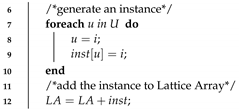 13 end 14 foreachinst in LAdo  33 end 34 returnC; |
- and are independent variables and dependent variables, respectively.
- Lines 5–13 aim to generate Lattice Array.
- Lines 16–22 aim to substitute real values for in and G and, hence, eliminate the independent variables. It is obvious that instances will simplify the computation of proposition (5).
- Lines 14–33 are a ForEach loop, hence, the algorithm is easy to parallelize.
- To make Algorithm 1 simpler, we can use to take the place of , the upper bound of , which is not allowed for theorem proving, as is crucial to theorem proving by CIM. However, for invariant generation, it only means we need to verify the obtained constraint in the second phase (Section 4).
Complexity Analysis
4. Illustration of CIM
- Guessing a template of fixed degree as an invariant template.
- Defining the complete inductive conditions.
- Applying a lattice array to the complete inductive conditions to generate the constraint on the parameters
- Solving the constraint. Any solution to the constraint guarantees the template an inductive invariant
- Applying Algorithm 1. We get three simpler implications and three corresponding R by Lemma 3 (Table 2).
- By Algorithm 1, is a constant, the consequent of implication is R, i.e., , and the constraint equations are . We will use this solution to simplify the remaining eight implications and the same below. Thus, the resulting implications become more and more simple (Table 4), we call it the domino effect, which is the benefit of parallelism in CIM.
- By Algorithm 1, and is the constraint equation. However, by comprehensive Gröbner basis, we need to compute the remainder under two situations: and . If is polynomial, situation becomes very complicated. This is why Sankaranarayanan et al. defined Alternative Consecution Relations to eliminate template variables in the antecedent of implication to avoid construction of comprehensive Gröbner basis. However, every coin has two sides. In Wu–Ritt’s Algorithm, means non-degenerate condition is false, the solution to may or may not satisfy the formula (5), which is crucial to the theorem’s proof by CIM. Fortunately, for invariant generation, it only means we need another step to verify the obtained invariant. Generally, verifying invariants is less expensive than generating invariants.
- By Algorithm 1, is a constant, so and . We continue to simplify the implications(Table 5).
- By Algorithm 1, and the constraint is , continue to simplify the implications(Table 6).
5. A Special Case
- For the initial condition case, it is same as Step 1.
- For the discrete consecution case (with ), assume that are dependent variables, are independent variables, and the size of lattice array is (2+1, 2+1).
- For the continuous consecution case (with ), there are no dependent variables as is ignored, are independent variables, and the size of lattice array is (2+1, 2+1,2+1).
- Solving these 37 implications, the following two groups of constraints are obtained:
6. Experiments
6.1. Experiment 1
6.2. Experiment 2
7. A Clever Use of CIM
8. Conclusions
- Applying instances by essentially instantiating the free variables to real numbers. Hence, the free variables are removed.
- Comparing to the existing approaches, CIM can solve the complete inductive conditions directly and is a complete approach.
- According to our analysis, Wu–Ritt’s method has exponential complexity while Gröbner basis method has double exponential complexity. Therefore, our approach is more efficient.
- Parallelization is another advantage of CIM. CIM was created to be a parallel method. To raise the computer’s calculation capacity, one important method is to develop both parallel machines and parallel algorithms.
Author Contributions
Funding
Conflicts of Interest
References
- Henzinger, T.A. The theory of hybrid automata. Available online: https://pub.ist.ac.at/~tah/Publications/the_theory_of_hybrid_automata.pdf (accessed on 10 April 2020).
- Alur, R. Formal verification of hybrid systems. In Proceedings of the 2011 Ninth ACM International Conference on Embedded Software (EMSOFT), Taipei, Taiwan, 9–14 October 2011; pp. 273–278. [Google Scholar]
- Sankaranarayanan, S.; Sipma, H.B.; Manna, Z. Constructing invariants for hybrid systems. Form. Methods Syst. Des. 2008, 32, 25–55. [Google Scholar] [CrossRef] [Green Version]
- Kong, H.; He, F.; Song, X.; Hung, W.N.; Gu, M. Exponential-condition-based barrier certificate generation for safety verification of hybrid systems. In Proceedings of the 25th International Conference on Computer Aided Verification (CAV2013), Saint Petersburg, Russia, 13–19 July 2013; pp. 242–257. [Google Scholar]
- Alur, R.; Dill, D.L. A theory of timed automata. Theor. Comput. Sci. 1994, 125, 183–235. [Google Scholar] [CrossRef] [Green Version]
- Henzinger, T.A.; Kopke, P.W.; Puri, A.; Varaiya, P. What’s decidable about hybrid automata? J. Comput. Syst. Sci. 1998, 57, 94–124. [Google Scholar] [CrossRef] [Green Version]
- Bogomolov, S.; Donzé, A.; Frehse, G. Guided search for hybrid systems based on coarse-grained space abstractions. Int. J. Softw. Tools Technol. Transf. 2015, 18, 1–19. [Google Scholar]
- Bogomolov, S.; Frehse, G.; Grosu, R. A box-based distance between regions for guiding the reachability analysis of SpaceEx. In Proceedings of the 24th International Conference on Computer Aided Verification (CAV 2012), Berkeley, CA, USA, 7–13 July 2012; pp. 479–494. [Google Scholar]
- Kong, H.; Bartocci, E.; Henzinge, T.A. Reachable Set Over-Approximation for Nonlinear Systems Using Piecewise Barrier Tubes. In Proceedings of the 30th International Conference on Computer Aided Verification (CAV2018), Oxford, UK, 14–17 July 2018; pp. 449–467. [Google Scholar]
- Tiwari, A. Abstractions for hybrid systems. Form. Methods Syst. Des. 2008, 32, 57–83. [Google Scholar] [CrossRef] [Green Version]
- Bogomolov, S.; Herrera, C.; Muniz, M. Quasi-dependent variables in hybrid automata. In Proceedings of the 17th Int. Workshop on Hybrid Systems: Computation and Control, Berlin, Germany, 15–17 April 2014; pp. 93–102. [Google Scholar]
- Bogomolov, S.; Schilling, C.; Bartocci, E. Abstraction-based parameter synthesis for multiaffine systems. In Proceedings of the 11th Haifa Verification Conference (HVC 2015), Haifa, Israel, 17–19 November 2015; pp. 19–35. [Google Scholar]
- Bogomolov, S.; Frehse, G.; Greitschus, M. Assume-guarantee abstraction refinement meets hybrid systems. In Proceedings of the 10th Haifa Verification Conference (HVC 2014), Haifa, Israel, 18–20 November 2014; pp. 116–131. [Google Scholar]
- Boreale, M. Algorithms for exact and approximate linear abstractions of polynomial continuous systems. In Proceedings of the 21st ACM International Conference on Hybrid Systems: Computation and Control, Porto, Portugal, 11–13 April 2018; pp. 207–216. [Google Scholar]
- Kong, H.; Bogomolov, S. Safety Verification of Nonlinear Hybrid Systems Based on Invariant Clusters. In Proceedings of the 20th ACM International Conference on Hybrid Systems: Computation and Control, Pittsburgh, PA, USA, 18–20 April 2017; pp. 163–172. [Google Scholar]
- Zhang, J.; Yang, L.; Deng, M. The parallel numerical method of mechanical theorem proving. Theor. Comput. Sci. 1990, 74, 253–271. [Google Scholar] [CrossRef] [Green Version]
- Zhang, J.; Lu, Y. Principles of parallel numerical method and single-instance method of mechanical theorem proving (in Chinese). J. Math. Pract. Theory 1989, 1, 36–45. [Google Scholar]
- Rodríguez-Carbonell, E.; Tiwari, A. Generating Polynomial Invariants for Hybrid Systems. In Proceedings of the 8th International Workshop on Hybrid Systems: Computation and Control, Zurich, Switzerland, 9–11 March 2005; pp. 590–605. [Google Scholar]
- Cachera, D.; Jensen, T.; Jobin, A.; Kirchner, F. Inference of polynomial invariants for imperative programs: A farewell to gröbner bases. Sci. Comput. Program. 2014, 93, 89–109. [Google Scholar] [CrossRef]
- Roux, P.; Voronin, Y.L.; Sankaranarayanan, S. Validating numerical semidefinite programming solvers for polynomial invariants. Form. Methods Syst. Des. 2018, 53, 286–312. [Google Scholar] [CrossRef] [Green Version]
- Tiwari, A.; Khanna, G. Nonlinear systems: Approximating reach sets. In Proceedings of the 7th International Workshop on Hybrid Systems: Computation and Control, Philadelphia, PA, USA, 25–27 March 2004; pp. 171–174. [Google Scholar]
- Prajna, S.; Jadbabaie, A. Safety verification of hybrid systems using barrier certificates. In Proceedings of the International Workshop on Hybrid Systems: Computation and Control, Philadelphia, PA, USA, 25–27 March 2004; pp. 271–274. [Google Scholar]
- Johnson, T.T.; Mitra, S. Invariant synthesis for verification of parameterized cyber-physical systems with applications to aerospace systems. In Proceedings of the AIAA Infotech at Aerospace Conference, Boston, MA, USA, 19–22 August 2013; p. 4811. [Google Scholar]
- Gulwani, S.; Tiwari, A. Constraint-based approach for analysis of hybrid systems. In Proceedings of the 20th International Conference on Computer Aided Verification, Princeton, NJ, USA, 7–14 July 2008; pp. 190–203. [Google Scholar]
- Sassi, B.; Amin, M.; Girard, A.; Sankaranarayanan, S. Iterative computation of polyhedral invariants sets for polynomial dynamical systems. In Proceedings of the 53rd IEEE Conference on Decision and Control (IEEE CDC2014), Los Angeles, CA, USA, 15–17 December 2014; pp. 6348–6353. [Google Scholar]
- Liu, J.; Zhan, N.; Zhao, H. Computing semi-algebraic invariants for polynomial dynamical systems. In Proceedings of the 11th International Conference on Embedded Software (EMSOFT 2011), Taipei, Taiwan, 9–14 October 2011; pp. 97–106. [Google Scholar]
- Boreale, M. Complete Algorithms for Algebraic Strongest Postconditions and Weakest Preconditions in Polynomial ODE’S. In Proceedings of the 44th International Conference on Current Trends in Theory and Practice of Informatics, Krems, Austria, 29 January–2 February 2018; pp. 442–455. [Google Scholar]
- Gallo, G.; Mishra, B. Wu-Ritt Characteristic Sets and Their Complexity. Discret. Comput. Geom. 1991, 6, 111–136. [Google Scholar]
- Ritt, J.F. Differential Algebra; American Mathematical Society: Providence, RI, USA, 1950. [Google Scholar]
- Wu, W. On the decision problem and the mechanization of theorem-proving in elementary geometry. Sci. China 1978, 29, 117–138. [Google Scholar]
- Wu, W. Basic principles of mechanical theorem proving in elementary geometries. J. Autom. Reason. 1986, 2, 221–252. [Google Scholar]
- Gallo, G. and Mishra, B. Efficient algorithms and bounds for Wu-Ritt characteristic sets. Eff. Methods Algebr. Geom. 1991, 94, 119–142. [Google Scholar]
- Alur, R.; Courcoubetis, C.; Halbwachs, N.; Henzinger, T.A. The algorithmic analysis of hybrid systems. Theor. Comput. Sci. 1995, 138, 3–34. [Google Scholar] [CrossRef] [Green Version]
- Maler, O.; Manna, Z.; Pnueli, A. From timed to hybrid systems. In Proceedings of the REX workshop 1991, Mook, The Netherlands, 3–7 June 1991; pp. 447–484. [Google Scholar]
- Alur, R.; Henzinger, T.A. Modularity for timed and hybrid systems. In Proceedings of the 8th InInternational Conference on Concurrency Theory (CONCUR 1997), Warsaw, Poland, 1–4 July 1997; pp. 74–88. [Google Scholar]
- Lygeros, J.; Tomlin, C.; Sastry, S. Controllers for reachability specifications for hybrid systems. Automatica 1999, 35, 349–370. [Google Scholar] [CrossRef]
- Floyd, R.W. Assigning meanings to programs. In Proceedings of the Amer. Math. Soc. Symp. in Applied Mathematics, Providence, RI, USA, 5–7 April 1967; pp. 19–32. [Google Scholar]
- Hoare, C.A.R. An axiomatic basis for computer programming. Commun. ACM 1983, 12, 53–56. [Google Scholar] [CrossRef]
- Wu, W.T. Mathematics Mechanization: Mechanical Geometry Theorem-Proving, Mechanical Geometry Problem-Solving, and Polynomial Equations-Solving; Kluwer Academic Publishers: Norwell, MA, USA, 2001. [Google Scholar]
- Cox, D.; Little, J.; O’Shea, D. Ideals, varieties, and algorithms. Am. Math. Mon. 1994, 101, 582–586. [Google Scholar]
- Weispfenning, V. Comprehensive gröbner bases. J. Symb. Comput. 1992, 14, 669–683. [Google Scholar] [CrossRef] [Green Version]
- Dubé, T.W. The structure of polynomial ideals and gröbner bases. Siam J. Comput. 1990, 19, 750–773. [Google Scholar] [CrossRef] [Green Version]
- Sharma, R.; Gupta, S.; Hariharan, B.; Aiken, A.; Liang, P.; Nori, A.V. A data driven approach for algebraic loop invariants. In Proceedings of the 22nd European Conference on Programming Languages and Systems, Rome, Italy, 16–24 March 2013; pp. 574–592. [Google Scholar]
- Padhi, S.; Sharma, R.; Millstein, T. Data-driven precondition inference with learned features. ACM Sigplan Not. 2016, 51, 42–56. [Google Scholar] [CrossRef]
- Collins, G. Quantifier elimination for real closed fields by cylindrical algebraic decomposition. In Proceedings of the 2nd GI Conference on Automata Theory and Formal Languages, Kaiserslautern, Germany, 20–23 May 1975; pp. 134–183. [Google Scholar]


| 0 | 0 | |
| 0 | 1 | |
| 0 | ||
| 1 | 0 | |
| 1 | 1 | |
| 1 |
| R | ||
|---|---|---|
| 0 | ||
| 1 | ||
| 2 |
| y | Implication | |
|---|---|---|
| 0 | 0 | |
| 0 | 1 | |
| 0 | 2 | |
| 1 | 0 | |
| 1 | 1 | |
| 1 | 2 | |
| 2 | 0 | |
| 2 | 1 | |
| 2 | 2 |
| y | ||
|---|---|---|
| 0 | 0 | |
| 0 | 1 | |
| 0 | 2 | |
| 1 | 0 | |
| 1 | 1 | |
| 1 | 2 | |
| 2 | 0 | |
| 2 | 1 | |
| 2 | 2 |
| y | ||
|---|---|---|
| 0 | 0 | |
| 0 | 1 | |
| 0 | 2 | |
| 1 | 0 | |
| 1 | 1 | |
| 1 | 2 | |
| 2 | 0 | |
| 2 | 1 | |
| 2 | 2 |
| y | ||
|---|---|---|
| 0 | 0 | |
| 0 | 1 | |
| 0 | 2 | |
| 1 | 0 | |
| 1 | 1 | |
| 1 | 2 | |
| 2 | 0 | |
| 2 | 1 | |
| 2 | 2 |
| Name | Alternative Discrete Consecution Condition |
|---|---|
| LC | |
| CV | |
| CS | |
| PS |
| Name | Alternative Continue Consecution Condition |
|---|---|
| LC | |
| CV | |
| CS | |
| PS |
| i | s | t | |||
|---|---|---|---|---|---|
| 0 | 0 | 1 | 1 | 1 | 0 |
| 1 | 1 | 2 | 3 | 1 | 0 |
| 2 | 3 | 3 | 6 | 1 | 0 |
| 3 | 6 | 4 | 10 | 1 | 0 |
© 2020 by the authors. Licensee MDPI, Basel, Switzerland. This article is an open access article distributed under the terms and conditions of the Creative Commons Attribution (CC BY) license (http://creativecommons.org/licenses/by/4.0/).
Share and Cite
He, H.; Wu, J. A New Approach to Nonlinear Invariants for Hybrid Systems Based on the Citing Instances Method. Information 2020, 11, 246. https://doi.org/10.3390/info11050246
He H, Wu J. A New Approach to Nonlinear Invariants for Hybrid Systems Based on the Citing Instances Method. Information. 2020; 11(5):246. https://doi.org/10.3390/info11050246
Chicago/Turabian StyleHe, Honghui, and Jinzhao Wu. 2020. "A New Approach to Nonlinear Invariants for Hybrid Systems Based on the Citing Instances Method" Information 11, no. 5: 246. https://doi.org/10.3390/info11050246