Abstract
The paper focuses on what two different types of Recurrent Neural Networks, namely a recurrent Long Short-Term Memory and a recurrent variant of self-organizing memories, a Temporal Self-Organizing Map, can tell us about speakers’ learning and processing a set of fully inflected verb forms selected from the top-frequency paradigms of Italian and German. Both architectures, due to the re-entrant layer of temporal connectivity, can develop a strong sensitivity to sequential patterns that are highly attested in the training data. The main goal is to evaluate learning and processing dynamics of verb inflection data in the two neural networks by focusing on the effects of morphological structure on word production and word recognition, as well as on word generalization for untrained verb forms. For both models, results show that production and recognition, as well as generalization, are facilitated for verb forms in regular paradigms. However, the two models are differently influenced by structural effects, with the Temporal Self-Organizing Map more prone to adaptively find a balance between processing issues of learnability and generalization, on the one side, and discriminability on the other side.
1. Introduction
What can computational modeling tell us about speakers’ word learning and processing? Simulations may provide a rigorous and testable conceptual framework within which one can analyze hypotheses for word learning and word processing. Lexical competence assumes the essential ability to retain sequences of symbolic units in the long-term memory, and access and retrieve them for language processing. From this perspective, computer simulations let one explore the relation between speakers’ behavior and general learning principles in detail.
For the present concern, the task of computational modeling the dynamic process of learning morphological competence can be dated back to Zellig Harris’s empiricist goal of developing linguistic analyses on the basis of purely formal and algorithmic manipulations of raw input data, to the commonly known discovery procedures [1]. Absence of classificatory information (e.g., morpho-syntactic or semantic information, annotation of morphological structure) in the training data qualifies the discovery algorithm as unsupervised. Conversely, when input word forms are associated with output information of some kind, then discovery is said to be supervised. In the first case, the task is modeled as a classification problem, in the second one, as a mapping issue.
Actually, no single computational implementation can deal with the whole range of psycholinguistic and neurolinguistic evidence accrued so far on what we know of word-learning and -processing by human speakers. Word processing has been defined as the outcome of simultaneously activating patterns of lexical knowledge, which reflect distributional regularities at different linguistic levels (i.e., morphological, semantic and syntactic ones) (e.g., [2]). Recent neuro-anatomical evidence has shown the interconnection between memory, lexical learning and processing, with cortical areas involved in working memory tasks and language processing inducing a considerable overlapping of activation patterns ([3,4]).
Far from replicating the whole range of neurolinguistics functions that are in play with human language processing, simulations may suggest a computational answer to several word processing effects highlighted by behavioral data. Among these, the ability of speakers to generalize novel forms, or recognize unknown forms, on the basis of already memorized ones, as well as the probabilistic nature of speakers’ perception of word internal structures.
Here, the main goal is to focus on these aspects of human communicative ability. In particular, what two different types of Recurrent Neural Networks (RNNs), namely a recurrent Long Short-Term Memory (LSTM) and a recurrent variant of self-organizing memories (i.e., a Temporal Self-Organizing Map, or TSOM), can suggest about the ways speakers learn and process a set of fully inflected verb forms selected from the top-frequency paradigms of two different languages, namely Italian and German.
Such input sets of inflected verb forms out of context do not represent a real human language acquisition context. However, experimental results will show how the specific properties of the inflectional systems influence the learning strategies adopted by the two neuro-biologically inspired models.
Recurrent LSTMs have been shown to be able to capture long-distance relations in time-series of symbols (e.g., [5,6,7]). TSOMs have recently been proposed to memorize symbolic time-series as chains of specialized processing nodes, which selectively fire when specific symbols are input in specific temporal contexts ([8,9,10,11]).
Both LSTMs and TSOMs can model lexical data as time-series of structured sequential data. The main goal in this paper is to evaluate learning and processing dynamics of verb inflection data in the two neural networks, for both Italian and German, by focusing on sensitivity to morphological structure, i.e., at the stem-affix boundaries, and on paradigm complexity.
The paper is organized as follows: related work is briefly introduced in Section 2. Section 3 is devoted to illustrating methods and materials that have been used for the experimental simulations. TSOM simulations are originally run; those with the recurrent LSTM refer to a previous work [12]. Newly approached analyses of results are detailed in Section 4, with a discussion developed in Section 5. A general conclusion is drawn in Section 6.
2. Related Work
RNNs appear to be the best architectural choice to deal with sequential data, as language-based data are, with recurrent connections that makes information cycling for a possibly long time (see, however, [5] for the gradient descent problem). Sequential data prediction has largely been the goal of statistical language modeling for predicting the ensuing word in a given context [13]. An important psycholinguistic model has been provided by [14], with sequential information encoded as sustained patterns of activation. Such an activation-based memory mechanism, with a recurrent connectivity, may account for short-term memory of serial order. This model has, however, received some criticism by [15] because of the item-order information that is encoded conjunctively, i.e., for any symbol occurring in a specific position the model assumes a different, specific representation.
Recurrent LSTMs have showed not only to be able to capture long-distance relations in sequential data, but also to avoid problems with training gradients, typical of simple Recurrent Networks (e.g., those based on the classic model proposed by Elman [16]).
In recent years, LSTMs have been applied for query autocompletion (e.g., [17]), or prediction tasks ([18,19,20], among many others).
Recently, a recurrent LSTM has been adopted to simulate word production as a cell-filling task [21], by training the model in different layer-size settings with morphologically complex lexeme families (noun lexemes for Russian, Finnish, Irish, and verb lexemes for Maltese and Khaling). A similar approach has been adopted in [12,22], where the task has been simulated by training a model with a set of inflected forms in verb paradigms, and tested on missing forms to be generated. Here, training consisted of lemma-paradigm cell paired with inflected form for all input forms. The approach has proved to be robust enough for a set of languages that show a gradient of morphological complexity (Italian and German in [12], and Italian, Spanish, German, English in [22]).
Finally, a recurrent variant of classical Kohonen’s Self-Organizing Maps (i.e., TSOMs), has been proposed as model of dynamic memories for lexical data. The authors in [11,23] have recently presented results on 6 inflection systems of different (in some cases typologically different) complexity (i.e., Arabic, Greek, Italian, Spanish, German, English), by focusing on learning and processing dynamics, rather than on a simple production task.
3. Materials and Methods
In this section, a detailed description of the datasets used for simulations is given, as well as a brief description of the two RNNs.
As anticipated, both LSTMs and TSOMs can model lexical data as time-series, thus allowing evaluation of learning and serial processing of verb inflection data by focusing on sensitivity to morphological structure.
3.1. The Data
Comparable sets of Italian and German inflected verb forms were selected by sampling the top-frequency 50 paradigms in two reference corpora ([24] for Italian, [25] for German). The choice of selecting the most frequent paradigms of the Italian and German verb systems has been done on the basis of data availability, and because they both offer evidence of graded levels of morphological irregularities with extensive allomorphy, including processing of prefixation (in German past participle only), vowel alternation, suppletion, suffixation.
A comparable set of paradigm cells has been defined for each of the 50 verb paradigms: specifically, the present indicative forms (n = 6), the past tense forms (n = 6), the infinitive form (n = 1), the past participle form (n = 1), and the present participle for German (n = 1), gerund form for Italian (n = 1). See details in Table 1.

Table 1.
The Italian and German datasets.
For each language, 695 forms have been used for training, and one or two forms for each paradigm, i.e., 55 forms, have been left out for testing. Due to the fact that not all inflected forms can be inferred from any others, the test sets for both languages have been defined according to a qualitative generalizable criterion, rather than on the basis of a quantitative leave-one-out cross-validation method. Testing forms have been selected on the basis of the degree of regularity of paradigms, according to the basic principle that they could be generalized on the basis of available training data: e.g., given the German forms for the present and past tense of finden (’find’), with their allomorph stems of, respectively, find- and fand-, the untrained past participle gefunden can hardly be generalized, unless the vowel-changing pattern (from i to a and u) is widely attested in many other irregular paradigms. Specifically, paradigms with inflected forms sharing the same stem, which is predictably realized starting from the verb root, are annotated as regular, while paradigms with more than one stem allomorphs, which undergo unpredictable formation, are classified as irregulars (following [26]).
3.2. The Neural Networks
LSTMs are RNNs that can process input data sequentially and keep their internal state through time, thus being able to learn long-term dependencies.
The functional architecture of the LSTM as adopted for training in [12] is given in Figure 1. Here, input vectors are encoded by dense matrices: a lemma, a set of morpho-syntactic features (i.e., tense, number, person, by including an extra dimension where a feature may not be attested, as for example for the present participle where there is no person/number), and a sequence of symbols (one at a time) are encoded as one-hot vectors. Input vectors are encoded by dense matrices whose outputs are concatenated into the projection layer z(t), and mapped to the LSTM layer, together with the information that has been output at time t − 1 (recurrent dynamic). Symbols are encoded as mutually orthogonal one-hot vectors, which implies that each symbol is equally different from any other ones.
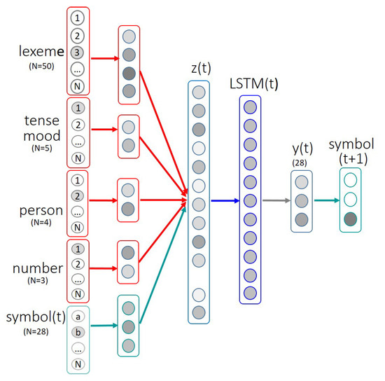
Figure 1.
Functional architecture of the recurrent LSTM. Input vector dimensions are given in parentheses. Inputs are mapped on the projection layer z(t) that is input to the recurrent layer LSTM(t). Adapted from [12].
A TSOM consists of a two-dimensional grid of memory/processing nodes that dynamically memorize input strings as chains of maximally responding nodes (Best Matching Units or BMUs). Each processing node has two layers of synaptic connectivity, an input layer connecting each node to the current input stimulus, and a re-entrant temporal layer, connecting each node to all map nodes. Every time a symbol is presented to the input layer, activation propagates to all map nodes through input and temporal connections, and the most highly activated node (BMU) is calculated. A functional architecture is sketched in Figure 2.
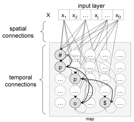
Figure 2.
Functional architecture of a Temporal Self-Organizing Map (TSOM). As an example, map nodes show the activation pattern for the input string #pop$. Directed arcs stand for forward Hebbian connections between BMUs. “#” and “$” are respectively the start and the end of input words.
For each BMU at time t, the temporal layer encodes the expectation for the BMU to be activated at time t + 1. The strength of the connection between consecutive BMUs is trained through principles of discriminative learning, for which, given an input bigram xa, the connection strength between the BMU that gets mostly activated for x at t and the BMU for a at t + 1 will increase if x often precedes a in training (dynamic of entrenchment) and decrease when a is preceded by a symbol other than x (dynamic of competition). Thus, during training, a TSOM gradually develops even more specialized sequence of BMUs for word forms—or sub-lexical chains—that are functionally dependent on the frequency distribution and the amount of formal redundancy in the training data. For a detailed description of learning equations see the Appendix in [11].
Once again, symbols are encoded as mutually orthogonal one-hot vectors (with a dimension of 28 bits for German, and 22 for Italian, including start-of-word and end-of-word symbols). The dimension of one-hot vectors is determined by the cardinality of different symbols that define the sets of input data. Symbols are the orthographical representations of word characters: to each orthographic character corresponds one symbol. The Italian data set is made up with 22 symbols, the German one with 28. This way of representation implies that, for example, vowels are not encoded as being more similar to one another, than to any of the consonants.
3.3. Training Protocol
The LSTM training experiment makes reference to [12]. There, training was stopped when the accuracy (i.e., the correct prediction of the ensuing character) stopped increasing at a defined threshold, for a maximum of learning epochs of 100. Both Italian and German datasets were administered for 10 times each to 256 and 512 LSTM blocks. For the present goal, I will consider only the best-performing configuration for each language, namely the 256-blocks for German and 512-blocks for Italian.
To replicate the same training protocol reported in [12], the TSOM has accordingly been trained for 100 learning epochs on each language. For each of the learning epochs, all forms have been randomly input to the TSOM 10 times each (token frequency = 10). Memory nodes are fitted on differences in cardinality of word forms (1764 for Italian, and 1600 for German). As I will show in the Results section, the behavior of the TSOM is more stable than those of the LSTM. Thus, only 5 repetitions of the same training session were run with identically parametrical settings to average results and control for random variability in the TSOM response.
4. Results
To produce/activate a fully inflected target form, both neural networks are prompted with a start-of-word symbol S1, which is used to predict the ensuing symbols S2 to Sn, until the end-of-word symbol is predicted.
4.1. Training and Test Accuracy
For the LSTM, the per-word accuracy is measured in terms of how many fully inflected forms are correctly produced, for both the training and test sets. For any wrongly produced symbol in a word, the whole word is considered to be inaccurately produced. Per-word scores are averaged across the 10 repetitions for each language (see details in Table 2).
Table 2.
Accuracy values for each language, neural network and training protocol. Standard deviations are given in parentheses.
In the TSOM, accuracy in learning (training) and generalization (test) is measured as the ability to recall any word from its internal memory trace. Accuracy values thus quantify the ability of a trained TSOM to retrieve any target form from its synchronic activation pattern. In the absence of an output level, accuracy in a TSOM is evaluated as the ability to activate the correct temporal chain of BMUs by propagating an integrated activation pattern representing the synchronic picture of the serial activation nodes. Recall errors on training sets are thus due to wrongly restored input sequences, as for example in the case of the Italian input chiamiamo, ’(we) call’, for which the TSOM activates the sequence of BMUs chiamo, and of German input gezeigt, ’shown’, for which the TSOM activates the sequence of geigt. As for the LSTM, a single wrongly retrieved symbol makes the whole word be considered to be inaccurately activated. See the 5 repetition-averaged results in Table 2.
Due to the basic architectural differences between LSTMs and TSOMs, accuracy values are related to a production task for the LTSM, and to a serial retrieving activation task for the TSOM. This may explain significantly different scores, for both the training and test datasets in both languages (statistical significance of t-test difference: p-value < 0.001).
In a TSOM, BMUs in themselves do not encode explicit timing information. However, during training, each node develops a dedicated sensitivity to both a possibly position-specific symbol and a context-specific symbol by incrementally adjusting its synaptic weights to recurrent patterns of morphological structure. Thus, a prediction task in a TSOM estimates its serial expectation for an upcoming symbol, and the evaluation of the map’s serial prediction accounts for modeling (un)certainty in serial word processing and perception of morphological complexity.
Likewise, the production task in the LSTM reveals its predictive nature, due to the re-entrant temporal connections, so that it can develop a sensitivity to upcoming symbols. Thus, monitoring per-symbol accuracy accounts for the network confidence about the next symbol to be output and perception of the morphological structure of fully inflected forms.
4.2. Prediction Scores
To focus on the dynamic sensitivity to morphological structure in the two networks, serial word processing has been evaluated for both LSTM and TSOM as the ability to predict a target word-form symbol-by-symbol.
Operationally, prediction in the LSTM is measured as the per-symbol accuracy in production. Conversely, the TSOM is prompted on the input layer with one symbol at a time, and the correctly expected BMU to be activated is verified.
I will consider two differently calculated prediction scores: (1) a purely anticipation score monitoring whether an upcoming symbol in a word is correctly produced/activated or not (i.e., for each matching output symbol is assigned a 1-score, for any non-matching ones a 0-score), and (2) an incrementally calculated prediction score (i.e., for each correct symbol a +1 point to the preceding score is assigned) accounting for a facilitatory/speeding effect in serial processing. Again, a wrongly predicted symbol is given a 0-point.
Accordingly, method (1) unfolds a structural effect, and method (2) reveals, for higher prediction scores, strong expectations over upcoming symbols reflecting both accurate positional symbol encoding and successful serial processing. Equations (1) and (2) indicate for LSTMs how prediction scores are calculated for each correctly produced symbol S(t + 1) at time t + 1. Conversely, for TSOMs, they are calculated for each correctly pre-activated/expected symbol.
4.3. Modeling Serial Processing
In the following subsections, I will show how prediction rates (calculated following both methods as described above) vary by modeling the time course of word processing with Generalized Additive Models, or GAMs, with regression plots (displayed with the ggplot function of the R software, cran.r-project.org) focusing on the interaction of the two differently calculated scores of prediction with the structural effect of the distance to the stem-ending boundary.
4.3.1. Prediction (1): Structural Effects
The idea here is to show a clear structural effect by exploring the statistical interaction of per-symbol prediction (according to Equation (1), namely whether the upcoming symbol is correctly anticipated or not) and the serial positioning of the specific symbol in context. In particular, I will consider the distance to the stem-suffix boundary for regular and irregular verb forms, at the end of the learning phase. In the regression plots reported in this and the ensuing sections, all verb forms are centered on the 0 of the x axis, representing the morpheme boundary, namely the first symbol of the inflectional ending. Accordingly, negative values on the xaxis mark the stems and positive values the suffixes.
The regression plots in Figure 3 illustrate the perception of morphological structure by the LSTMs trained with Italian and German sets and tested with the 55 untrained forms. Intuitively, the task is easier at the beginning of the stem in both Italian and German, with a reduced accuracy for irregular alternating stems (see solid lines in the 4 regression plots). For all the 4 GAMs, the difference between regular and irregular regressions is statistically highly significant (t-test, p-value < 0.001).
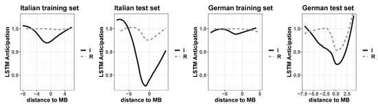
Figure 3.
Regression plots of interaction between morphological (ir)regularity (Regulars versus Irregulars) and distance to morpheme boundary (MB) in non-linear models (GAMs) fitting the number of correctly anticipated symbols by the trained LSTMs on Italian (left plots) and German (right plots) for training and test sets.
Accuracies drop to a minimum score around the morpheme boundary, namely at the stem-suffix transition (on the x axis −1 corresponds to the end of the stem, and 0 to the beginning of the inflectional ending), in particular for forms in irregular paradigms. The effect is more robust for the test set, for both Italian and German (confirmed by a greater proportion of explained deviance the GAM models output, or adjusted R2).
The evidence suggests that producing regulars is easier than irregulars, due to the presence of stem allomorphy in the latter. In particular, the more systematic/predictable the distribution of stem alternants, the easier the task. This is the case of German, with accuracy scores significantly higher than Italian ones (see Table 2) in both training (t-test, p-value < 0.001) and test (t-test, p-value < 0.05).
In addition, due to the existence of conjugation classes in Italian, based on the presence in most—but not all—paradigm cells of a thematic vowel, learning and generalization of inflectional endings is more difficult than inferring unattested suffixes for German, which in turn exhibits no conjugation classes and suffixes that are generally attested for both regulars and irregulars.
As claimed in Section 4.2, the task for a TSOM is slightly different. The anticipation rate takes into account whether the symbol at time t is correctly pre-activated by the map given the symbol at time t−1. In the case of TSOMs, the task is more related to a recognition task rather than to a production task, as in the case of LSTMs.
Figure 4 shows the regression plots for the trained TSOMs on both training and test sets for Italian (the left plots) and German (the two plots on the right side). As a general trend, being it a recognition task, as more symbols are processed, the TSOM gets more accurate in anticipating the ensuing symbols. In fact, since no morpho-syntactic information is given, neither during training nor for the prediction test, the more symbols are shown the easier for the TSOM to recognize the target word-form. However, the structural effect of morphological discontinuity is prominent.
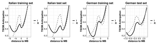
Figure 4.
Regression plots of interaction between morphological (ir)regularity (Regulars versus Irregulars) and distance to morpheme boundary (MB) in non-linear models (GAMs) fitting the number of correctly anticipated symbols by the trained TSOMs on Italian (left plots) and German (right plots) for training and test sets.
Interestingly enough, for both Italian and German, stems are easier to be anticipated/recognized in regular paradigms since all inflected forms share the same stem. However, this effect is offset by suffix selection, with a major drop for regulars than irregulars (see −1 on the x axis corresponding to the end of stems, and 0 corresponding to the first symbol of suffixes).
Stems in irregular paradigms, in fact, tend to be anticipated less easily since the allomorphic alternating patterns are not always fully predictable. The typical discontinuous pattern of morphological structure in irregular paradigms induces levels of anticipation that are, on average, lower than those for more regular paradigms (i.e., regular paradigms and those irregular ones that are highly predictable due to a widely attested alternating pattern, as for example for German bleib/blieb in bleiben ’stay’, schreib/schrieb in schreiben ’write’). However, stem allomorphs typically select only a subset of paradigm cells, i.e., they select only a few possible inflectional endings, thus favoring anticipation on suffix recognition.
Contrary to LTSMs, anticipation evidence by TSOMs suggests that structural effects are more evident for regulars, with a better perception of serial discontinuity (at the stem-suffix boundary) for more regular forms than irregular ones.
4.3.2. Prediction (2): Serial Processing Effects
An incrementally calculated prediction score (see Equation (2)) is designed to evaluate the processing ease in serial production and recognition. As briefly introduced in Section 4.2, the incremental measure highlights, for higher prediction scores, both accurate positional symbol encoding and successful serial processing.
The regression plots in Figure 5 emphasize that processing uncertainty for the LSTMs is extremely reduced when the dependent variable (i.e., symbol prediction) puts a premium on correctly predicted sequences of symbols. It is useful to recall that prediction scores are calculated by incrementally assigning each correctly anticipated symbol a +1 point, i.e., the score assigned to the preceding symbol incremented by 1 (see Equation (2)).
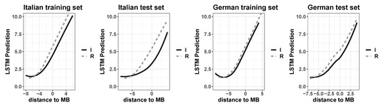
Figure 5.
Regression plots of interaction between morphological (ir)regularity (Regulars versus Irregulars) and distance to morpheme boundary (MB) in non-linear models (GAMs) fitting the incremental number of correctly predicted symbols by the trained LSTMs on Italian (left plots) and German (right plots) for training and test sets.
The structural effect highlighted in the previous section with the Boolean anticipation measure, namely the V-shape curve with a reduced accuracy at the morpheme boundary, tends to disappear here by showing almost linear regression curves. Nevertheless, the statistical highly significant difference in processing regular and irregular forms is confirmed for both Italian and German, and both training and test sets (t-test, p-value < 0.001). In addition, GAMs are highly explanatory, with values of adjusted R2 respectively of 85.5% and 70.1% for Italian training and test sets, and 88.6% and 68.0% for German sets, although the variance is fairly high for all sets (i.e., for each serial position, values for the prediction task in the LSTM are highly dispersed from the mean). Precisely, for both languages and both training and test sets, GAMs fitted symbol prediction with distance to the morpheme boundary (MB), word length, and morphological (ir)regularity as fixed effects, with distance to the MB and word length as smooth effects in addition.
Concerning the TSOM, as stated in Section 3.2, dynamics of entrenchment and competition define the final organization of a trained map as a function of the frequency distribution and the amount of formal redundancy in the training data. For highly redundant data, such as inflected forms in verb paradigms, a TSOM will specialize, with a strong inter-node connectivity, highly responding BMUs to highly attested sub-patterns, as, for example, for stems shared by many inflected forms (i.e., in more regular paradigms). Conversely, less specialized BMUs are less strongly, though more densely, connected to any other nodes, thus meeting the input of more word forms.
The regression plots in Figure 6 confirm the trend of differently distributed processing costs for regulars and irregulars (respectively, dashed and solid lines in the plots), with prediction values higher for the former than the latter (for Italian and German training sets, t-test, p-value < 0.001). However, this is statistically not significant for the German test set.
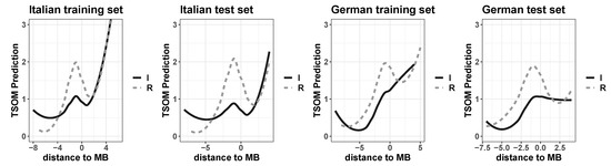
Figure 6.
Regression plots of interaction between morphological (ir)regularity (Regulars versus Irregulars) and distance to morpheme boundary (MB) in non-linear models (GAMs) fitting the incremental number of correctly predicted symbols by the trained TSOMs on Italian (left plots) and German (right plots) for training and test sets.
Once again, the stem-suffix boundary (for positions at −1 and 0 on the x axis) marks a cutting drop in prediction values for forms in regular paradigms, emphasizing the intuition that when a whole stem is recognized/predicted, the TSOM has to update its expectations for an upcoming suffix. The more forms share the same substring before that discontinuity point, i.e., the same stem, the greater this effect, for both the training and test sets in both languages.
For German, the update of expectations for upcoming suffixes is more delayed than for Italian forms, due to the full formal nesting of shorter inflectional endings with longer ones (e.g., -e, -en, -end, as for example in mache, machen, machen, (I) ’do’, (we/they) ’do’, ’doing’), which makes it difficult to predict up to the end-of-word forms in the absence of contextual/morpho-syntactic information, and when it is not biased by real frequency distributions. Both architectures are, in fact, administered with a uniform distribution of inflectional data to factor out token frequency effects and focus on the effects of morphological structure only. In detail, in the LSTM each form was shown once per epoch; in the TSOM each form has been input 10 times per epoch.
Conversely, irregulars tend to exhibit a different pattern. Here, in fact, the initial disadvantage in processing alternating stems is counterbalanced by a smaller effort for the selection of the inflectional endings. This is due to the reduction of processing uncertainty at the stem-suffix boundary, since each stem allomorph selects only a subset of all attested suffixes. Ultimately, the serial processing for irregulars appears to be more linear and exhibit a reduction in structural discontinuity. This is particularly clear for the German sets, where irregulars tend to blur the TSOM sensitivity to the morphological structure, thus favoring a more holistic processing strategy.
5. Discussion
The predictive nature of the production/recognition task in both LSTM and TSOM, due to the re-entrant layer of temporal connectivity in both architectures, makes them develop a strong sensitivity to sequential patterns that are highly attested in the training data. Since both recurrent neural networks are designed to take into account the sequentiality of input data, they can both deal with context-sensitivity issues.
Both algorithms are fairly good in learning from training data, showing to be effective in inferring novel inflected forms based on cumulative evidence coming from memorized verb forms. Thus, the main focus has been on monitoring per-symbol accuracy to model the networks’ confidence about the next symbol to be output (in production) or input (in recognition) and the effects of morphological structure of fully inflected forms on word processing.
For both LSTM and TSOM, training data consist of unsegmented verb forms. However, as shown in the Results section, the two models develop a good perception of structural discontinuity at the stem-suffix boundary, which is differently apportioned across word forms depending on morphological (ir)regularity.
All in all, the evidence for both the LSTM and the TSOM shows that respectively, production and recognition are facilitated for verb forms in regular paradigms, and that generalization is easier for untrained forms in regular paradigms than irregular ones. However, contrary to LTSMs, prediction evidence by TSOMs suggests that structural effects are more evident for regular forms, with a better perception of serial discontinuity, in particular at the stem-suffix boundary.
Due to the differently implemented and conceptualized task of prediction for the two architectures, evidence coming from the two networks provides different pieces of information.
For the trained LSTMs, I suggest that accuracy in prediction is properly interpreted as ease of serial production, showing that LSTM is effectively able to infer novel forms on the basis of evidence of trained verb forms. However, this ability strongly interacts with morphological redundancy: in fact, regularly inflected forms are easily learnt, more than irregular ones, and they offer good evidence for untrained forms to be efficiently generalized (see Section 4.3.1 and Figure 3). Regression models show how easily the LSTMs can produce upcoming symbols of forms in regular paradigms, namely with reduced uncertainty compared to irregular ones. This is statistically significant for both training and test sets, for both Italian and German, with an effect that is even greater for the test sets. This confirms that LSTM’s efficiency in inferring novel forms from trained data is significantly higher when more verb forms share the same stem, and the task of generalizing untrained forms is based on highly predictable patterns (i.e., the same stem shared by all members of the same paradigm family, and suffixes attested in many other paradigms).
Conversely, for irregular forms, the task is more difficult and serial production shows the profile of processing uncertainty around the morpheme boundary. Irregular paradigms are in fact characterized by less predictable forms, based on alternating, possibly suppletive stems.
Such a trend is far more prominent for Italian than for German, with the former being more complex than the latter. Degrees of morphological complexity may be seen in the overall learning accuracies for Italian and German, in both training and test sets, with Italian being a more inflectionally complex system than German (see [27]).
The incremental measure of prediction (see Equation (2)), by putting a premium on more symbols that are correctly serially produced, tends to minimize the impact of morphological (ir)regularity on word production. Although statistically significant, the advantage of regular forms is reduced compared to irregular ones. In fact, for both regulars and irregulars, the more symbols are input, the more likely they are to be correctly produced (see the almost linear regression lines in Figure 5). Here, the incremental measure more clearly emphasizes the real nature of production that includes word planning.
By contrast, evidence coming from the trained TSOMs shows how processing ease strongly interacts with word structure. The transparent and systematic nature of regular verb forms induce the TSOM to clearly recognize stems more easily than irregular forms may do. The facilitatory effect of having all forms in the paradigm that activate the same stem is strong enough to speed up serial prediction with both measures (see Figure 4 and Figure 6). On the contrary, alternation and unpredictability in stem formation cause irregular forms to slow down TSOM prediction before the morpheme boundary. The more stem allomorphs a paradigm presents, the larger the effort taken to process them and to generalize untrained forms.
However, the small number of inflected forms in irregular stem families (i.e., the subset of forms sharing the same stem in an irregular paradigm) reduce uncertainty for suffix selection. The initial disadvantage in recognizing irregular stems is counterbalanced by a smaller effort in predicting the following suffix. Due to the well-known correlation between morphological irregularity and frequency ([28]), this effect would be even greater by considering real token frequency distributions.
Thus, the effect of structural discontinuity is greater in processing regulars than irregulars, with the latter showing a more linear prediction (especially with measure (2)). This is the case of German irregular forms (see Figure 6), with suffixes that are on average shorter than Italian ones.
Finally, production and recognition show to be differently affected by morphological (ir)regularity. On the one side, production, as implemented in the LSTM, is strongly favored by regularity, since lexical redundancy and transparent predictability enhance word-learning and generalization of unknown forms. The memory trace of an invariant stem that is transparently shared by all its paradigmatically related forms receives frequency support from all these forms. Accordingly, it is perceptually more salient and thus more easily extended to unknown forms.
On the other side, the task of recognition, as implemented in the TSOM architecture, shows a less sharp effect, as it is facilitated in processing a regular stem, but somewhat slowed down in identifying the inflectional endings of regularly inflected forms. These apparently conflicting results are in fact in line with the functional requirements of a complex communicative system like verb inflection. An adaptive and open system is in fact maximally functional to generalizing novel forms, and must be comparatively easy to learn; conversely, a maximally contrastive system of irregular forms would take the least effort to process, but would require full storage of unpredictable items, thus turning out to be slower to be learnt. An efficient system must strike a dynamic balance between these two requirements.
These results give support to the evidence presented by contrasting serial and parallel processing ([29]): a word supported by a dense neighborhood (i.e., many members of the same family) is produced/read faster. However, when the same word is presented serially, as for example in a task of spoken word recognition, high-frequency neighbors engage in competition and inhibit processing.
6. Conclusions
Psycholinguistic evidence shows how prediction and competition based on word similarity and lexical redundancy affect speakers’ anticipation of incoming stimuli, speed input recognition and improve lexical decision (see [30,31]).
From this perspective, the main contribution of this paper has been to show how two different RNNs (i.e., LSTM and TSOM) may address issues of word-learning, generalization of untrained forms, and perception of morphological structure, without being exposed to morpheme segmentation.
By varying the calculus of the prediction task, the two RNNs show an overall facilitatory effect of morphological regularity to learning and processing, with some qualifications.
The LSTM architecture proves to be more effective in planning the task of prediction, and to be less influenced by effects of serial uncertainty. It clearly shows what happens when a system must deal with learning and processing regular and irregular verb forms.
Conversely, the TSOM model proves to be more sensitive to morphological structure, namely to morpheme patterns that are shared by more verb forms, which emerge during learning as fundamental units of structural processing. With no information about the morpho-syntactic features during training, lexical structures are emerging from purely formal redundancy in surface input data, and lexical organization is grounded in memory-based processing strategies only. It thus suggests how learning and emergence of morphological structure is possible on a purely perceptual/surface level.
Funding
This work partially received support by POR CReO FESR 2014-2020, SchoolChain project, grant number D51B180000370009.
Acknowledgments
The present methodological analysis stems from simulations and reviewing work jointly conducted within the Comphys Lab, www.comphyslab.it. I do thank three anonymous reviewers for their insightful comments on a first version of the present paper.
Conflicts of Interest
The author declares no conflict of interest.
Abbreviations
The following abbreviations are used in this manuscript:
| RNN | Recurrent Neural Network |
| LSTM | Long Short-Term Memory |
| TSOM | Self-Organizing Map |
| BMU | Best Matching Unit |
| MB | Morpheme Boundary |
References
- Harris, Z. Methods in Structural Linguistics; University of Chicago Press: Chigaco, IL, USA, 1951. [Google Scholar]
- Post, B.; Marslen-Wilson, W.; Randall, B.; Tyler, L.K. The processing of English regular inflections: Phonological cues to morphological structure. Cognition 2008, 109, 1–17. [Google Scholar] [CrossRef] [PubMed]
- D’Esposito, M. From cognitive to neural models of working memory. Philos. Trans. R. Soc. Biol. Sci. 2007, 362, 761–772. [Google Scholar] [CrossRef] [PubMed]
- Ma, W.J.; Husain, M.; Bays, P.M. Changing concepts of working memory. Nat. Neurosci. 2014, 17, 347–356. [Google Scholar] [CrossRef] [PubMed]
- Bengio, Y.; Simard, P.; Frasconi, P. Learning long-term dependencies with gradient descent is difficult. IEEE Trans. Neural Netw. 1994, 5, 157–166. [Google Scholar] [CrossRef] [PubMed]
- Hochreiter, S.; Schmidhuber, J. Long short-term memory. Neural Comput. 1997, 9, 1735–1780. [Google Scholar] [CrossRef] [PubMed]
- Jozefowicz, R.; Zaremba, W.; Sutskever, I. An empirical exploration of recurrent network architectures. In Proceedings of the 32nd International Conference on Machine Learning (ICML-15), Lille, France, 6–11 July 2015; pp. 2342–2350. [Google Scholar]
- Ferro, M.; Marzi, C.; Pirrelli, V. A self-organizing model of word storage and processing: Implications for morphology learning. Lingue Linguaggio 2011, 10, 209–226. [Google Scholar]
- Marzi, C.; Ferro, M.; Nahli, O. Arabic word processing and morphology induction through adaptive memory self-organisation strategies. J. King Saud Univ. Comput. Inf. Sci. 2017, 29, 179–188. [Google Scholar] [CrossRef]
- Pirrelli, V.; Ferro, M.; Marzi, C. Computational complexity of abstractive morphology. In Understanding and Measuring Morphological Complexity; Baerman, M., Brown, D., Corbett, G., Eds.; Oxford University Press: Oxford, UK, 2015; pp. 141–166. [Google Scholar]
- Marzi, C.; Ferro, M.; Pirrelli, V. A processing-oriented investigation of inflectional complexity. Front. Commun. 2019, 4, 1–48. [Google Scholar] [CrossRef]
- Cardillo, F.A.; Ferro, M.; Marzi, C.; Pirrelli, V. How “deep” is learning word inflection? In Proceedings of the 4th Italian Conference on Computational Linguistics, Rome, Italy, 1–12 December 2017; pp. 77–82. [Google Scholar]
- Mikolov, T.; Karafiát, M.; Burget, L.; Černockỳ, J.; Khudanpur, S. Recurrent neural network based language model. In Proceedings of the 11th Annual Conference of the International Speech Communication Association, Chiba, Japan, 26–30 September 2010; pp. 1045–1048. [Google Scholar]
- Botvinick, M.; Plaut, D.C. Short-term memory for serial order: A recurrent neural network model. Psychol. Rev. 2006, 113, 201–233. [Google Scholar] [CrossRef] [PubMed]
- Bowers, J.S.; Damian, M.F.; Davis, C.J. A fundamental limitation of the conjunctive codes learned in PDP models of cognition: Comment on Botvinick and Plaut (2006). Psychol. Rev. 2009, 116, 986–997. [Google Scholar] [CrossRef] [PubMed][Green Version]
- Elman, J.L. Finding structure in time. Cogn. Sci. 1990, 4, 179–211. [Google Scholar] [CrossRef]
- Jaech, A.; Ostendorf, M. Personalized language model for query auto-completion. arXiv 2018, arXiv:1804.09661. [Google Scholar]
- Gers, F.A.; Schmidhuber, E. LSTM recurrent networks learn simple context-free and context-sensitive languages. IEEE Trans. Neural Netw. 2001, 12, 1333–1340. [Google Scholar] [CrossRef] [PubMed]
- Ghosh, S.; Vinyals, O.; Strope, B.; Roy, S.; Dean, T.; Heck, L. Contextual LSTM (CLSTM) models for large scale NLP tasks. arXiv 2016, arXiv:1602.06291. [Google Scholar]
- Xu, K.; Xie, L.; Yao, K. Investigating LSTM for punctuation prediction. In Proceedings of the 10th International Symposium on Chinese Spoken Language Processing (ISCSLP), Tianjin, China, 17–20 October 2016; pp. 1–5. [Google Scholar]
- Malouf, R. Generating morphological paradigms with a recurrent neural network. San Diego Linguist. Pap. 2016, 6, 122–129. [Google Scholar]
- Cardillo, F.A.; Ferro, M.; Marzi, C.; Pirrelli, V. Deep Learning of Inflection and the Cell-Filling Problem. Ital. J. Comput. Linguist. 2018, 4, 57–75. [Google Scholar]
- Marzi, C.; Ferro, M.; Nahli, O.; Belik, P.; Bompolas, S.; Pirrelli, V. Evaluating inflectional complexity crosslinguistically: A processing perspective. In Proceedings of the Eleventh International Conference on Language Resources and Evaluation (LREC 2018), Miyazaki, Japan, 7–12 May 2018; pp. 3860–3866. [Google Scholar]
- Lyding, V.; Stemle, E.; Borghetti, C.; Brunello, M.; Castagnoli, S.; Dell’Orletta, F.; Dittmann, H.; Lenci, A.; Pirrelli, V. The paisá corpus of italian web texts. In Proceedings of the 9th Web as Corpus Workshop (WaC-9)@ EACL, Gothenburg, Sweden, 26 April 2014; pp. 36–43. [Google Scholar]
- Baayen, H.R.; Piepenbrock, P.; Gulikers, L. The CELEX Lexical Database; Linguistic Data Consortium, University of Pennsylvania: Philadelphia, PA, USA, 1995. [Google Scholar]
- Aronoff, M. Morphology by Itself: Stems and Inflectional Classes; The MIT Press: Cambridge, MA, USA, 1994. [Google Scholar]
- Bittner, D.; Dressler, W.U.; Kilani-Schoch, M. Development of Verb Inflection in First Language Acquisition: A Cross-Linguistic Perspective; Mouton de Gruyter: Berlin, Germany, 2003. [Google Scholar]
- Wu, S.; Cotterell, R.; O’Donnell, T.J. Morphological Irregularity Correlates with Frequency. In Proceedings of the 57th Annual Meeting of the Association for Computational Linguistics, Florence, Italy, 28 July–2 August 2019; pp. 5117–5126. [Google Scholar]
- Chen, Q.; Mirman, D. Competition and Cooperation Among Similar Representations: Toward a Unified Account of Facilitative and Inhibitory Effects of Lexical Neighbors. Psychol. Rev. 2012, 119, 417–430. [Google Scholar] [CrossRef] [PubMed]
- Balling, L.W.; Baayen, R.H. Morphological effects in auditory word recognition: Evidence from Danish. Lang. Cogn. Process. 2008, 23, 1156–11902. [Google Scholar]
- Balling, L.W.; Baayen, R.H. Probability and surprisal in auditory comprehension of morphologically complex words. Cognition 2012, 125, 80–106. [Google Scholar] [CrossRef] [PubMed]
Sample Availability: Datasets are available from the author. |


© 2020 by the author. Licensee MDPI, Basel, Switzerland. This article is an open access article distributed under the terms and conditions of the Creative Commons Attribution (CC BY) license (http://creativecommons.org/licenses/by/4.0/).