Abstract
In the dynamic vehicle routing problem with mixed backhauls (DVRPMB) both pick up orders and delivery orders, not related to each other, are served. The requests of the former arrive dynamically while the latter are known a priori. In this study, we focus on the case of limited fleet, which fulfills all delivery orders, but may not have enough capacity to serve all pick up orders within the available working horizon. The problem’s dynamic nature and the attention to customer service raise interesting considerations, especially related to the problem’s objectives. The problem is solved through periodic re-optimization, acknowledging the fact that this pseudo-dynamic approach may lead to some limitations. For the underlying (static) optimization problem we propose appropriate objective functions, which account for vehicle productivity and propose a branch-and-price (BP) approach to solve it to optimality. The results indicate how the performance of the various objectives is impacted by different re-optimization frequencies and policies in this practically relevant environment of dynamic demand served by a limited fleet. Specifically, extensive experimentation indicates that accounting for vehicle productivity within a typical periodic re-optimization solution framework may result to higher customer service under a range of operational settings, in comparison to conventional objectives.
1. Introduction and Background
In the dynamic vehicle routing problem with mixed backhauls (DVRPMB) a fleet of vehicles originating from a depot is tasked to serve two types of orders: (i) static orders known prior to the start of operations (typically deliveries); and (ii) dynamic pickup orders, which are received in real time and should be collected and returned to the depot for further processing. Typically, there exists an initial routing plan (a-priori plan) that assigns the static (delivery) orders to the available fleet, while dynamic orders received during plan execution must be assigned to appropriate vehicles in real time. The problem’s scope is to serve all static orders and allocate all dynamic ones to the vehicles en route or to extra vehicles available at the depot in order to minimize the overall routing costs.
The variant of DVRPMB with limited number of vehicles is studied in the present work, termed the DVRPMB with limited resources (m-DVRPMB). This is a problem of significant value since the constraint of resources is relevant in most practical problems. The problem’s dynamism is addressed through periodic re-optimization. It should be emphasized, however, that due to the resource constraints some of the newly received dynamic orders may not be served, raising interesting considerations that are discussed below.
The first of these considerations relates to the objective function of the optimization problem solved at each re-optimization cycle. As it will be demonstrated, conventional objectives that account strictly for either cost minimization or service maximization are either inappropriate or may not address the problem effectively. In particular, cost minimization is not appropriate. This is because serving dynamic orders increases cost and under the cost minimization objective these orders will be left unserved. On the other hand, if service maximization is sought, the process of solving the underlying optimization problem repeatedly within the re-optimization framework may prove to be greedy, leading eventually to serving less orders during the entire horizon (see Section 5.3). Another related consideration in this setting of limited resources concerns client prioritization at each re-optimization cycle. Specifically, during re-optimization it may be beneficial to favor serving certain dynamic customer orders (e.g., urgent ones) over others, under the assumption that the low priority (e.g., not urgent) ones may fit in the plan during a subsequent re-optimization cycle.
In previous work [1], the authors have studied the DVRPMB without resource constraints (i.e., under unlimited fleet) and applied a re-optimization strategy that re-optimizes the plan at certain time instances considering the new information that becomes available. For the re-optimization problem, the authors proposed a branch-and-price (BP) approach to obtain exact solutions, as well as a column generation-based insertion heuristic to address challenging cases (e.g., without time windows). Regarding the re-optimization process, two related issues was investigated: (a) the re-optimization policy (frequency), i.e., when to re-plan and (b) the implementation tactic, i.e., what part of the new plan to commit for execution and communicate to the drivers. Regarding the latter, it was concluded that the recommended tactic is to commit for execution only those dynamic orders scheduled for implementation prior to the next re-optimization cycle (partial release tactic, PR). Using the PR tactic, re-optimization upon arrival of each dynamic order provides for maximum efficiency. In subsequent work [2], these authors examined a variant of the DVRPMB problem in [1] that allows orders to be transferred between vehicles during plan implementation, again without considering resource constraints.
Despite the practical importance of limited resources (vehicles), m-DVRPMB has not been addressed in the literature. If all orders to be served are known in advance, the re-optimization problem of m-DVRPMB is similar to the pickup and delivery problem with selective pickups (PDPSP) [3,4,5], which is a very interesting and practical problem of the more generic Pickup and Delivery VRP [6,7,8,9,10]. In PDPSP, all deliveries must be performed, but pick-ups are optional; however, pick-ups generate a profit when collected. The objective is to minimize the routing costs minus the collected revenue. This problem arises naturally in reverse logistics contexts, in which customers return goods (e.g., empties) to the depot.
The PDP with selective pickups was first addressed in [3] for a single vehicle. The authors used an exact branch-and-bound technique to solve it by employing flow variables and adaptations of the well-known Miller–Tucker–Zemlin constraints ([11]) in order to prevent subtours. Their approach was able to solve instances of up to 30 customers. In [12] a branch-and-cut algorithm was proposed, able to solve instances of up to 90 customers. The authors in [13] developed heuristic methods to study a practical problem, which involved the delivery of soft drinks to convenience stores in the city of Quebec and the collection of empties (bottles or cans) using a heterogeneous fleet of vehicles. In their problem formulation, pick-ups were associated with revenue and they could be performed only if they did not violate vehicle capacity constraints.
The authors in [14] studied the routing of supply vessels to offshore installations, in which vessels pick-up empty containers. In this problem, due to limited capacity, it is not always possible to serve all collections and, thus, priority is given to the most important ones. The authors formulated the problem as a mixed integer linear program and they were able to solve practical instances with 10 installations to optimality using CPLEX 9.0. The work in [15] studied a similar application and proposed a tabu search method to solve the single vehicle pick-up and delivery problem with selective pick-ups. More recently, an exact branch-and-price algorithm has been proposed in [5] for the vehicle routing problem with deliveries, selective pickups and time windows (VRPDSPTW), in which instances of up to 50 customers were solved to optimality for five variants of this problem.
The m-DVRPMB is also part of the general category of dynamic vehicle routing problems (DVRPs; [16]), which have attracted an increasing body of research over the last two decades. In dynamic (and deterministic) routing problems, basic information is gradually revealed over time. Commonly used strategies for solving such problems is (a) to re-optimize the plan whenever the available information changes, a strategy often referred to as reactive approach [17,18] or (b) at fixed intervals, also referred to as periodic re-optimization ([19,20]). In the former approach, a full re-optimization can be performed when there is adequate time to calculate the updated solution. However, given that this is not feasible in most practical applications, periodic approaches are more commonly employed since the re-optimization effort is known in advance (due to the fixed intervals). Certain strategies have been proposed to improve periodic re-optimization, such as: buffering and waiting [21]. The waiting strategy (see, e.g., [22]) aims at minimizing the travel time of the vehicles by waiting as long as possible prior to heading to the next destination or drive immediately (and, eventually, wait at this destination if required). In a buffering strategy, a certain number of requests is expected to be received prior to re-optimization or the least urgent request is postponed until the latest possible time (see [1,21]).
Typically, there are three solution directions that can be found in the literature; (a) local update procedures, in which simple policy-based techniques (heuristics) are used to incorporate the new requests in the current plan as in [23,24]; (b) exact algorithms or metaheuristics to reoptimize the entire solution while considering all up-to-date information as in [19,25,26] and (c) advanced methods that exploit the nature of the underlying dynamic problem, using for example, diversion ([27]) or waiting strategies ([22,28]). For further insights in dynamic routing, the interesting reader may refer to the work of [29,30,31,32,33] and the surveys of [34,35].
An appropriate concern is the problem’s objective function. Most studies on dynamic routing are based on reactive approaches and assume that it is possible to serve the demand completely; hence, they typically focus on minimizing the number of vehicles and the routing costs. Only a few studies focus on fleet resource constraints and the possibility of rejecting requests [36]. It is noted that while in many practical dynamic logistics applications rejecting a request is not permitted, since it may harm company reputation and customer satisfaction, there are many other applications in which customer demand may not be served completely. Thus, problems with fleet constraints and partial demand service are of considerable practical interest.
Based on the existing literature reviewed above and the practical significance of the problem addressed, the contributions of the current work include the following:
- Concerning the underlying static optimization problem of the m-DVRPMB: It is similar, but not identical, to the PDP with selective pickups. In the former: (a) there is no revenue associated with pick-up orders; and (b) there are vehicles stationed at the depot that may be used to serve (some of) the increased load caused by the newly arrived requests. This re-optimization problem is being solved by extending the heuristic branch-and-price (BP) approach proposed in [1], to address the fleet constraint;
- A more interesting—and original—aspect of the work stems from the dynamic nature of m-DVRPMB. Based on the intrinsic features of the problem, two primary questions arose (a) is there an appropriate objective function that considers service maximization in anticipation of additional work not yet known; (b) how does the fleet constraint affect the performance of the re-optimization frequency?
- To address the first research question, this study proposes and studies alternative objective functions that maximize service, while, at the same time, enhance vehicle productivity. Vehicle productivity is a newly introduced term that encourages the available fleet to complete as much of the known work as early as possible. The performance of those proposed objective functions is compared to a conventional objective function that accounts only for service maximization, by deploying a series of experiments that consider various operating scenarios and parameters;
- The second research question is concerned with how the limited fleet constraint affects the trends related to the performance of the various re-optimization strategies, i.e., a combination of when to re-optimize and which part of the plan is released for implementation. This is investigated through appropriate experimentation.
The remainder of this paper is structured as follows: Section 2 presents the problem more formally, as well as the framework proposed to solve the DVRPMB with limited resources. Section 3 discusses the objective functions for m-DVRPMB and sets the related theoretical foundation. Section 4 presents the model for m-DVRPMB structured in a way that makes it amenable to a branch-and-price approach; the proposed approach is also presented in this section. Section 5 investigates experimentally the effect of the proposed objective functions on the efficiency of the solution under different problem settings. Finally, Section 6 summarizes the key findings of this work and opportunities for further research.
2. Problem Description and Solution Framework
2.1. Problem Description
Consider a transportation network in a Euclidean plane. A limited fleet of homogeneous vehicles (set ), each with limited capacity is located at a single depot prior to the start of operations. At the beginning of the planning horizon , a set of vehicles commence the execution of their planned routes to serve a set of static delivery orders known in advance, while is the set of vehicles that remain at the depot. A vehicle, once dispatched, is required to return to the depot by . During the execution of the distribution plan, new customers call-in, requesting pickup services. These arriving orders (hereafter denoted dynamic orders, DO) must be collected and returned to the depot. Static (delivery) orders originally assigned to vehicles cannot be re-allocated to other vehicles, while DO may be served by any vehicle as needed.
A typical objective of the problem would be to maximize the number of served customers throughout the available shift, while reducing the total cumulative routing cost. A feasible solution of the problem should serve all static orders (while there is no such requirement for DO) and should respect customer and driver shift time windows (TW). Furthermore, the total load of the vehicle cannot exceed the vehicle’s capacity at any time.
2.2. Solution Framework
The allocation of DO to the fleet vehicles is dealt through periodic re-optimization (see Figure 1). It is assumed that in the overall planning horizon there will be re-optimization cycles, each corresponding to an appropriate “static” problem , with re-optimization occurring at time instances where . Re-optimization cycles ( ) may or may not be of equal duration. The “static” problem solved at each re-optimization time considers all information known up to the related point in time. It is assumed that problem is solved instantaneously.
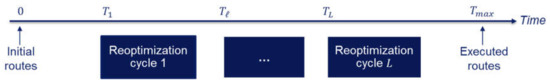
Figure 1.
Re-optimization process.
A re-optimization problem takes into account two sets of orders not yet served: (i) the committed orders (denoted as set ), which include all orders assigned to a vehicle originally or during previous re-optimization cycles—These orders have not been served and cannot be re-allocated to other vehicles; and (ii) the flexible orders (denoted as set ), which correspond to newly arrived DO or previously arrived DO not yet served—These may be reassigned to any vehicle . As in the work of [1], depending on the release tactic followed, two scenarios are relevant: (a) committed orders correspond only to static orders and flexible orders are all DO not yet served (partial release scenario, PR); and (b) committed orders are all orders assigned to vehicles during any previous cycle and not yet served; flexible orders correspond only to newly arrived DO (full release scenario, FR). Let also denote the set of all orders involved in a re-optimization cycle and represent the set of all nodes; that is, committed orders (), flexible orders (), starting location of all vehicles (set ) and the depot ().
It should be noted that within this context, it is assumed that a DO left unplanned at a certain re-optimization cycle, can be reconsidered during subsequent re-optimizations cycles. This assumption follows the practice of some courier companies, in which the available call-center accepts all incoming requests (given that there is no access or visibility to the planning system) and only at a later stage informs the customer in case they are not able to satisfy their request.
In practice, the solution framework of Figure 1 may be implemented using current communication and information technologies. Requests arriving in real time through a call-center are used as inputs into the planning system. The dispatcher chooses a certain re-optimization policy, and an appropriate part of the resulting plan is transmitted to the drivers via on-board devices cellphones or PDAs.
The solution of the static problem of re-optimization cycle considers the entire remaining time horizon . Part of this solution is then implemented until the next re-optimization time . The following assumptions concerning the operational scenario are also considered: (i) The current state of the logistics system is assumed to be known at any time; (ii) vehicles must arrive at customers before the end of their time–window; in case vehicles arrive prior to the time window’s opening, they wait until the window opens; (iii) the route is updated only at customer locations, i.e., diversion is not permitted (as, e.g., in [17]); (iv) in case a vehicle completes its route prior to the end of working horizon (), then it is allowed to wait at the location of the last customer.
As mentioned earlier, due to the resource constraints in m-DVRPMB, some of the newly received dynamic orders may not be served. This renders the application of conventional objectives unsuitable and makes the re-optimization problem quite different from that of DVRMB and quite interesting. For instance, if service maximization is sought, the process of solving the underlying optimization problem repeatedly within the re-optimization framework may prove to be greedy, leading eventually to serving less orders during the entire horizon. Of course, such objective may still be applicable in cases in which probabilistic information for future events is incorporated in the planning as in [31,37,38]. However, many environments in practice do not use forecasting information, hence the need to make decisions based strictly on the information at hand is crucial. For such cases, the current study proposes and studies alternative objective functions that maximize service, while, at the same time, enhance vehicle productivity.
2.3. The Mathematical Model of the Problem
The mathematical model of the static version of the re-optimization problem for the m-DVRPMB is based on the formulation proposed in [1], which focuses solely on minimizing the total cumulative routing costs. In order to account for the fleet limitation, this model is modified in two ways: (a) the objective function was re-designed to address the unique characteristics of the problem as discussed in Section 3 and (b) the branch-and-price formulation was revised appropriately, as discussed in Section 4. It is noted that the problem constraints are typical to the ones of a VRPTW formulation. In particular, they comprise route continuity constraints, vehicle capacity constraints and time constraints (i.e., order time windows and available working horizon). Section 4 and Appendix A elaborate on those constraints, in view of the column generation-based formulation of the re-optimization problem. More details on the mathematical formulation of m-DVRPMB can be found in [39].
3. Objective Functions for the Re-Optimization Problem of m-DVRPMB
This section introduces three objective functions to deal with limited resources in the context of the re-optimization problem: (a) a conventional one that maximizes service by assigning a fixed profit to each DO served (objective ); (b) an objective that provides additional profit for each order (static or dynamic) served within the next (upcoming) re-optimization cycle (objective ); and (c) an objective that provides profit for all orders to be served at any future period; in this case, however, the profit decreases linearly depending on the period (re-optimization cycle) the respective order is being served (objective ).
Let denote the fixed profit assigned to each served DO and the additional profit in case an order (static or dynamic) is served within the upcoming re-optimization cycle; then, the profit per order corresponding to the three (3) alternative objective functions varies as illustrated in Figure 2. By using the appropriate function, the solution method may be steered into maximizing customer service (objective ) or vehicle productivity (objectives and ). Section 3.1 and Section 3.2 describe the structure of the proposed objective functions.
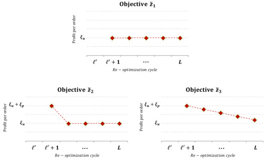
Figure 2.
Profit per order for the three objectives.
It should be noted that for objectives and to be relevant, re-optimization must take place at predefined time intervals known a priori (e.g., once per hour). Re-optimization policies that depend on the number of arrived DO may be only implemented under objective .
3.1. A Conventional Objective Function that Maximizes Service
The objective function of DVRPMB with an unlimited fleet strictly minimizes routing cost. As mentioned previously, under this objective if the constraint for serving all orders is relaxed in the re-optimization problem, then (in general) no dynamic order will be included in the final solution, since serving it will increase routing cost. To address this issue, one can introduce additional (profit) terms in the objective function to simultaneously:
- Increase the number of DO served throughout the remaining horizon—primary objective
- Decrease the total cumulative routing costs (over the remaining horizon)—secondary objective
That is,
where is the set of arcs connecting all nodes of ; i.e., . Furthermore, denote binary flow variables equal to if arc is traversed by vehicle and zero otherwise. denotes the cost of traversing arc .
Under an appropriately large positive value of , this objective maximizes the number of served DO and among the solutions with the maximum DO number it selects the one with minimum routing cost. should be set to a value that exceeds the upper bound of the cost (worst case) of incorporating a DO in the current plan. This can be achieved by setting to a value larger than , where represents the cost of the unit route .
Objective may be appropriate for a static planning problem with limited resources (for which all orders are known a priori) but may not be adequate in the setting under study since additional orders are expected to arrive. The anticipation of additional work favors reserving fleet capacity for the latter periods of the operational horizon so that newly arriving DO may be served. This, in turn, indicates that the available fleet should complete as much of the known work as early as possible (i.e., increase the productivity of the system in the earlier re-optimization cycles), in order to reserve capacity for later re-optimizations.
There are multiple ways that fleet productivity and thus the capacity of the system to serve new DO, may be impacted adversely by objective , especially during early re-optimization cycles, in which the few DO known up to that point may all fit in the plan. In these early cycles, using (a) may cause the incorporation of DO by consuming significant resource availability (e.g., include one or more DO at significant detour cost(s), despite the fact that the DO service is due much later in time); (b) some vehicle(s) may be forced to wait for long periods at customer sites for a TW to open, since it may be more cost-efficient to assign a DO with late opening time when a vehicle is closer to it (see also example in Figure 3); (c) vehicles stationed at the depot may not be used, since it may be more cost-efficient to assign a DO to a vehicle already en route.
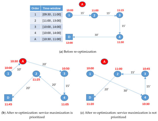
Figure 3.
Example: comparing possible alternative expressions of objective (A is the newly received dynamic order; 1, 2, 3, 4 represent the committed orders; D is the depot). (a) Before re-optimization; (b) After re-optimization: service maximization is prioritized; (c) After re-optimization: service maximization is not prioritized.
All these potentialities may significantly decrease the productivity of the fleet at the early re-optimization cycles when all DO may fit in the plan. However, neglecting entirely the routing costs in an attempt to increase fleet productivity is also not appropriate, since an excessive increase of costs in the current re-optimization cycle may shift work towards the subsequent (future) re-optimization cycles.
Based on these considerations, the objective function is enhanced below in order to maximize productivity of the fleet appropriately in the upcoming re-optimization cycle(s), in anticipation of additional work to come, without excessively burdening the capacity of the system at later re-optimization cycles.
3.2. Objective Functions That Account for Vehicle Productivity
An enhanced objective function is proposed, which in addition to maximizing the total number of DO served, it attempts to maximize the number of orders served within the upcoming re-optimization cycle (the length of which is known in advance); it does so, however, among the solutions with the same number of DO served (i.e., in a lexicographic order). Consider the re-optimization problem during the -th cycle and let denote a decision variable that is equal to if order is served during the time interval by vehicle and otherwise. Then, the proposed objective function (denoted as ) seeks the following in lexicographic order:
- Maximize the number of dynamic orders () served throughout the remaining horizon;
- Maximize the number of both static and dynamic orders () served within the upcoming re-optimization cycle (i.e., within time interval );
- Minimize the routing cost.
In (2) corresponds to a positive value (profit) if an order is served within the time interval (of known duration); weights the part of objective that minimizes the routing cost.
Although the primary goal of objective is to maximize the DO served throughout the horizon, term (b) favors increased fleet productivity during the current cycle in anticipation of additional work to come. Specifically, with this term we attempt to encourage the deployment of resources as early as possible, even if this results in higher routing costs. This is particularly useful in the early re-optimization cycles, in which all DOs may be served. In this case, term (a) of the objective function assumes the same value for all solutions. As a consequence, term (b) will select the solution that serves the greatest number of orders during the current cycle, resulting in the positive impact discussed above.
However, prioritizing term (a) over term (b) in the objective function is also important in such a dynamic context, since it is uncertain if a DO not included in the solution of the current re-optimization cycle can be served at a later stage. For solutions under the FR tactic those DO that are not included in the solution of the current re-optimization cycle are not considered during future ones. For solutions under PR tactic (in which not all DO fit in the plan), prioritizing term (a) over (b) ensures that the objective will not force serving more orders (static and dynamic) during the interval at the expense of including a DO in the current plan.
To better illustrate the latter case, consider the example of Figure 3a, which presents the state of a single route at the re-optimization time instance . At time , the vehicle is located at customer 1 and is scheduled to serve three static orders (2, 3 and 4), while dynamic order A needs to be incorporated in the current plan (with time window opening at ). The expected time of arrival to each order (prior to re-optimization and incorporation of order A), as well as the travel duration of each planned arc are also displayed in figure. (Note that in this case the vehicle arrives at customer 1 at 10:00, but waits for 45 min, due to the opening of the time window of customer 2.) Furthermore, assume that . If we prioritize term (a) over term (b) in this example, the objective will attempt to maximize the number of orders served within time interval among the solutions that incorporate order A. The result of this scenario is illustrated in Figure 3b, in which order A has been incorporated in the plan and one static order (order 3) has also been served till the next re-optimization time (i.e., ). Figure 3c illustrates the opposite, i.e., when term (a) is not prioritized over term (b). It is clear from Figure 3c that dynamic order A will remain unplanned, since due to the objective, the preferred solution is the one that serves the three static orders (2, 3 and 4) during interval [10:00,11:00] (i.e., one more order will be served during this interval compared to solution of Figure 3b). Order A may not be served since its time window has elapsed.
To force the primacy of term (a) of the objective over term (b), the following should hold:
Note that the largest possible value of the right hand side of (3) is obtained if all remaining orders (of set ) are served in the next re-optimization cycle (i.e., . Thus, in Equation (3) can be written as:
This may be satisfied with:
where ε is a small positive real number. Working along the same lines, in order to guarantee the primacy of term (b) over term (c), the value of should be larger than the largest possible value of the routing cost, i.e.,
This routing cost value (upper bound) can be assumed when all orders are included in the solution and they are served directly from the depot, since each order can be served exactly once and the fleet is homogeneous. Thus, in Equation (6) can be reduced to:
Assuming and replacing based in Equation (5), we have:
This may be satisfied by:
Using in the values of Equations (5) and (9) will ensure that from those solutions that maximize the number of served DO, the one to be selected (a) serves as many orders as possible in the interval (; and (b) has the minimum routing cost among the ones serving the same number of orders in this interval.
As already discussed, forcing as many orders as possible to be served until time may cause higher routing costs, compared to scenarios in which orders may be served at an appropriate time. Objective function , already mentioned above, moderates this effect by encouraging orders to be served early, but even beyond . Objective has a similar structure to that of objective , but assigns to each served order a revenue that decreases linearly depending on the period (re-optimization cycle) the order is served (as in Figure 2).
In particular, consider a DVRPMB instance with re-optimization cycles of known duration and the solution of the re-optimization problem during cycle . Let denote the re-optimization cycle in which order is served and denote the profit obtained by serving order during time interval , . Then profit is provided by the following Equation:
Then, objective is obtained by replacing profit with . Note that objectives and reduce to objective if and .
4. Branch and Price Model and Solution Approach for the Re-Optimization Problem of m-DVRPMB
The underlying re-optimization problem of m-DVRPMB is modeled and solved by modifying appropriately the branch-and-price (BP) framework proposed in [1] for the DVRPMB. In BP, a MILP problem is solved using the column generation (CG) method by relaxing the integrality constraints of the original problem and solving the resulting large linear program within a Branch and Bound (BB) tree (see [40,41,42]).
The BP framework for the re-optimization problem of m-DVRPMB is presented in this section by describing the set-partitioning model, the column generation solution approach and the overall Branch and Bound scheme. In this description, the index (which denotes the re-optimization cycle) is omitted, since the problem has the same form for any cycle.
4.1. A Set-Partitioning Formulation for the Re-Optimization Problem of m-DVRPMB
The master problem (MP) for the re-optimization problem of m-DVRPMB is formulated as a set partitioning problem (SPP), in which each column corresponds to a feasible route and each constraint corresponds to a customer been served. Let denote the set of orders served by route , where refers to the set of all feasible routes. Let be a binary coefficient that takes the value 1 if order and let denote the routing cost of route . Finally, let reflect the revenue if order is served. For simplicity and without loss of generality, let and . Thus, the total cost of route for objective is given from:
For objective , the total cost is:
where denotes the re-optimization cycle (time interval) in which customer is served in route with . It should be noted that the total cost of route for objective is given from Equation (11) when and ; i.e., .
In the m-DVRPMB formulation, set of all feasible routes-columns comprises two subsets, i.e., , where columns correspond to vehicles en route and columns correspond to vehicles that are located at depot. Assuming coefficient equal to 1 if route is used in the solution and zero otherwise, the set partitioning problem related to the master problem of m-DVRPMB may be formulated as follows:
Objective Function (13) minimizes the total net cost of the selected routes. Constraint (14) ensures that each static order is served by exactly one vehicle, while constraints (15) state that each DO can be served at most once. Finally, constraint (16) limits the number of vehicles.
4.2. Column Generation Approach
In column generation, the relaxed Linear Programming version of the master problem (MP) is solved to optimality by sequentially solving restricted versions of it ([43]). The linear programming version of the problem (LMP) is achieved by replacing constraint (17) with .
The solution of LMP is addressed by iteratively solving a restricted version (RLMP) of the former, which considers a subset of variables (columns) and by identifying new columns to be added to . This is performed until no new columns can be identified.
More specifically, the initial set of feasible columns of the RLMP is generated as follows: (a) the set of columns is formed by exploiting the information resulting from solving re-optimization problem , when all orders that were served up to (i.e., during ) are eliminated; (b) the set of columns is formed by generating single-visit trips that originate and finish at the depot, i.e., . In order to check if there are any other columns (routes) than can further reduce the objective of the RLMP, the reduced costs of each non-basic route are calculated, as given by Equation (18):
where () are the shadow (dual) prices related to customer constraints (14)–(15) and () are the shadow (dual) prices related to resource constraints (16). In order to identify such variables (columns), a different optimization problem is solved (pricing sub-problem, SP). This problem handles all remaining constraints that a column (route) is required to satisfy.
Hence, the next step is to generate feasible routes with negative reduced cost that have not yet been included in the current RMP, along with their reduced costs . For the case addressed in this paper, independent sub-problems (SP) are being defined and solved, one for each vehicle en route (that will generate new columns ) and only one for the vehicles located at the depot; the latter will generate new columns . Each one of the subproblems considers orders (where denotes the committed orders assigned to vehicle ), while the subproblem considers orders .
Formulating and Solving the Pricing Sub-Problem (SP) in m-DVRPMB
The SP is modeled as an elementary shortest path problem with time windows and capacity constraints (ESPPTWCC). The objective of this SP is given by Equation (19) below by denoting as the modified cost associated with arc , that is .
where denotes a decision variable that is equal to if order is served during time interval , , where ( denoting the current re-optimization cycle) and 0 otherwise. Profit is calculated according to Section 3.2 (depending on the objective). The constraints involved in this problem ensuring feasibility of each route are given in Appendix A.
The SP is solved using the label correcting algorithm of [44,45] presented in [1]. Given the requirement for time efficiency of the solution process, the column-generation-based insertion heuristic presented in [1] is also employed; this heuristic uses various approaches for generating columns for the |K| subproblems (vehicles en route), as well as subproblem |K| + 1 (for the vehicles located at the depot). For the former, instead of solving each SP to optimality (which is the most time consuming part), the heuristic uses an insertion-based procedure that finds the minimal cost of inserting each one of the DO to each one of the available routes based on the dual prices generated on each iteration of the RMP. For the |K|+1 problem, an ESPPTWCC with more relaxed dominance criteria is solved to generate columns for the vehicles located at depot.
4.3. Branch and Bound
If no integer solutions are obtained by the CG algorithm, a branch-and-bound (B&B) search scheme is used ([40,41,42]). In this scheme, the CG algorithm computes lower bounds at each node of the B&B search tree and branches on the most fractional binary arc flow variable (see [41,46,47]). In addition, when the heuristic approach is applied, the B&B is executed for an upper time limit (e.g., 1 min); if the optimum integer solution has not been reached, the columns (routes) present in the current RMP are being used within an integer-programming solver (CPLEX) in order to obtain an efficient integer solution.
An important issue is validation of correct implementation before the deployment of the solution algorithm. While the original approach to address the underlying (static) problem at each re-optimization cycle is an exact one, the one deployed to address the computational efficiency requirements is a heuristic version of the exact approach that provides efficient solutions with an average deviation of around 2%. This performance was assessed through extensive experiments using the Solomon benchmarks [48]. The resulting performance is similar to the one observed for the unlimited fleet case (where all DO are served) in [1]. Concerning the framework within which solution of the static problem is employed, there are no comparable results in the literature against which the obtained results may be compared, since m-DVRPB was introduced in the current study.
5. Computational Experiments
To assess the performance of the above methods, an extensive experimental analysis was conducted. The problems employed and the metric used for evaluating the results are presented in Section 5.1. The experimentation is then presented in two sections, each one addressing different research questions. Section 5.2 investigates how the limited fleet constraint affects the performance of the various re-optimization strategies (combination of re-optimization policy and tactic mentioned in Section 1) when re-optimization is driven by the number of DO received. Obviously, in this part of the study only objective is employed since objectives and may only be used under a framework of predefined re-optimization times. Section 5.3 investigates the case of predefined re-optimization intervals in order to assess which objective function is preferable in each re-optimization strategy and under which operating scenarios. For all test instances, the heuristic version of the BP framework presented in Section 4 is used by allowing it to run for up to 60 s; if the optimal integer solution has not been reached then, the columns (routes) present in the current RMP are used within an integer-programming solver (CPLEX) in order to obtain an efficient integer solution.
An assessment of the performance of the BP heuristic with respect to its exact counterpart was also carried out. The findings have indicated that the BP heuristic yields efficient solutions with an average deviation of around 2%, a performance similar to the one observed for the unlimited fleet case (all DO served) in [1].
All experiments were implemented in Matlab® 7.14.0 (R2012a) using an Intel Core i7 PC System with processor speed 2.8 GHz and 4.00 GB of RAM running Windows 7®.
5.1. Experimental Setup
5.1.1. Test Instances
The R1 and C1 datasets of Solomon [48] (12 and 9 instances, respectively) were used for this experimental study. In addition, instances vrpnc8 and vrpnc14 of Christofides [49] were also employed, which do not include TW for the uniform and clustered cases, respectively, but use the same customer coordinates of R1 and C1 datasets. These instances are designated as R100 and C100, respectively. Table 1 summarizes the instances employed.

Table 1.
Test instances from Solomon and Christofides (for the instance designations see [49] and above).
Another factor investigated is how customer service is affected by fleet availability, i.e., by the number of extra vehicles stationed at the depot to serve DO. For each one of the 23 instances, the investigation considered three (3) cases of 0, 2 and 4 vehicles available at the depot (denoted as V-0, V-2, V-4, respectively). Figure 4 illustrates the average number of DO (as a percent of total) served per dataset (R1 and C1) for each case of vehicle availability at the depot, along with the minimum and maximum values. The percentages presented are the averages over all instances (and test problems) by assuming that all DO are known in advance (see Section 5.2).
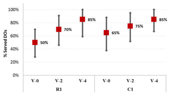
Figure 4.
Average percentage of DO served vs. the available vehicles at depot per dataset (for the designation of the experimental instances see above).
Thus, the experimentation considered a total of 69 different cases (3 × 23). For each case, a moderate degree of dynamism, dod (50% DO) was assumed and10 different problems were generated and used by a random selection of static orders among the order set. Thus, a total of 690 test problems were used in the experimental investigation. The initial solutions (original assignment of static orders to vehicles) were obtained by a Clark and Wright savings heuristic of [50] followed by the Reactive Tabu Search metaheuristic of [51] as a post-optimization process. Finally, DO are provided during the window according to a continuous uniform distribution.
5.1.2. The Assessment Metric Used
The performance of the proposed method is being assessed based on the so-called value of information (VoI) metric, which was originally introduced in [52]. This metric is enhanced in order to take into account both the number of DO served and the routing cost. Let denote the total number of DO served in the final solution of dynamic problem under objective and the corresponding total routing cost. Then, the objective function value for problem when solved under is:
Since the objective function results in negative values, the VoI used in this study is given by the following formula:
where denotes the value of the metric for the related static problem (in which all DO are known prior to the dispatching of the vehicles; i.e., at time ). It should be also noted that was set to 1000 throughout the experimental study (penalties and were calculated based on according to the Equations presented in Section 3.2).
5.2. Re-Optimization Driven by the Number of Dynamic Orders: Performance of Various Strategies
This section investigates the performance of the re-optimization strategies for the limited fleet case. As discussed in Section 1, a re-optimization strategy comprises the combination of re-optimization cycle timing (policy) and the part of the plan that is released for implementation (tactic). The experimental investigation employed re-optimization policies that depend on the number of DO received, which corresponds to a typical practice. Therefore, since the time instances (and the ensuing periods) of re-optimization are not known in advance, this analysis involved only objective .
All instances described in Section 5.1.1 were employed. The policies tested are re-optimization upon the arrival of each DO (SRR) and re-optimization upon the arrival of a predefined number of DO (NRR). For NRR, the values of (where is the total number of DO) were used, hereafter designated as NRR-1, NRR-2 and NRR-3. Each policy was tested under the full-release (FR) and partial-release (PR) tactics (see Section 1), resulting to a total of eight (8) strategies for each one of the 690 test problems (i.e., 5520 problems in total).
Figure 5 presents the performance (with respect to VoI) of each re-optimization strategy (policy-tactic combination) for each investigated dataset (R1 and C1), averaged over all test problems of the related dataset (and of course over all cases with respect to the number of vehicles available at the depot). Lower values of VoI indicate better performance (i.e., solutions closer to the respective static problem, where all DOs are known in advance). From this figure it is clear that (a) the SRR-PR strategy provides the best average performance (minimum VoI) and (b) the PR tactic outperforms FR (on the average) in all datasets. The performance difference between the two tactics decreases as the number of elapsed DO per re-optimization cycle increases (smaller number of re-optimization cycles). Furthermore, the PR tactic seems to be more efficient for shorter re-optimization cycles and the FR tactic seems to be less efficient when re-optimization is applied very frequently (SRR) or infrequently (NRR-3). The observed performance seems to agree with the behavior of the re-optimization strategies for the unlimited fleet case in [1], indicating that the performance of the strategies is not affected significantly by limiting the available resources.
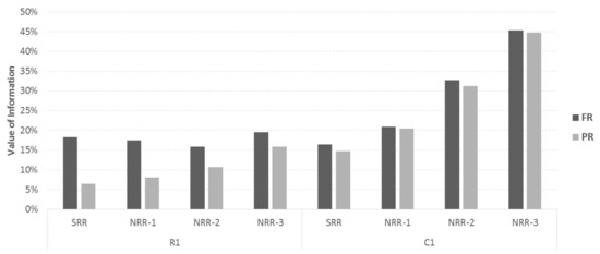
Figure 5.
Average performance of re-optimization strategies for the different datasets (SRR—single-request re-optimization; NRR—N-request re-optimization; R1—customers have a uniform geographical distribution; C1—customers are clustered).
The experimentation has also indicated similar patterns to those of Figure 5 with respect to the performance of re-optimization strategies for all values of fleet availability, i.e., there is no significant interaction between fleet availability and the re-optimization strategies on the average. Therefore, the detailed results are not presented here (but can be found in [1]).
5.3. Re-Optimization at Known Time Intervals: Performance of the Three Objectives
The performance of the three proposed objectives discussed in Section 3 is being assessed. This investigation includes all instances described in Section 5.1.1 for the R1 dataset (13 instances, including R100), under three values of fleet availability (V-0, V-2 and V-4) and using 10 different test problems per instance (i.e., 390 test problems in total).
As mentioned before, the fixed-time re-optimization (FTR) policies are employed, which comprise cycles of equal duration. In particular, four values of re-optimization frequency were used, i.e., every 10, 20, 40 and 60 units of time with respect to (which is equal to 230 units of time in the Solomon instances), hereafter designated as FTR-10, FTR-20, FTR-40 and FTR-60. Each policy was tested under the FR and PR release tactics, resulting to a total of eight (8) strategies for each one of the 390 test problems of R1 dataset (i.e., 3120 problems in total).
Figure 6 presents the performance (with respect to VoI of Section 5.1.2) of each objective for each investigated instance of the R1 dataset (incl. R100), averaged over all test problems and re-optimization policies and tactics. As before, lower values of VoI correspond to better performance. According to the figure, objectives and (which consider vehicle productivity) seem to provide more efficient solutions for cases with increasing TW width, compared to objective ; this improvement is more pronounced in cases with wide TW (R103, R104, R107, R108) or no time windows (R100).
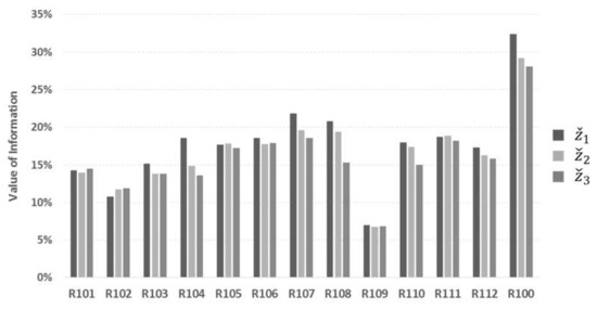
Figure 6.
Overall average performance of objectives per investigated instance.
This trend may be attributed to the fact that wide (or no) TWs allow for more customer combinations and, thus, more opportunities for customers to be served sooner (e.g., till the next re-optimization cycle). In addition, objectives and keep vehicles busy, delaying their return to the depot. This allows for increased opportunities when new orders are considered in subsequent cycles. On the other hand, and do not seem to favor cases with limited TW width (e.g., R101, R102, R105). In those cases, the TW limitation for serving a DO decreases the possibilities of including future DO in the plan. This fact, in combination with the expected increase of routing costs under objectives and , may cause the performance to deteriorate compared to objective .
Figure 7 illustrates the performance of the three objectives with respect to re-optimization strategies (policy and tactic combination), averaged over all test instances and values of vehicle availability. Based on the figure, the performance under objectives and improves in the FR tactic. This is expected, since using (and thus not accounting for vehicle productivity) under the FR tactic, may schedule the service of newly received DO way into the future in the expense of significant resources, e.g., time (especially for newly dispatched vehicles from depot). This is not the case with and , which tend to use the vehicles en route as much as possible given the current information and the additional work to come.
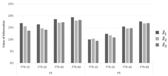
Figure 7.
Average performance of objectives with respect to re-optimization policy and tactic (FTR—fixed-time re-optimization; FR—full-release tactic; PR—partial-release tactic).
Another interesting takeaway from Figure 7 is that objective seems to lead to more efficient solutions when re-optimization is applied more frequently (see FTR-10 and FTR-20 cases). This may be attributed to the fact that a higher number of re-optimization cycles allows to allocate the DO to the appropriate period. On the other hand, objective performs slightly better in cases of longer re-optimization intervals.
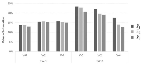
Finally, the experimental study examined the interaction of different values of vehicle availability and different TW patterns (the latter characterized by the ratio of the average TW width of all customers with respect to ). This was carried out by grouping all instances in two categories, as shown in Table 2.
Table 2.
Classification of investigated instances in TW-pattern groups based on TW width (% of ).
Figure 8 presents the average performance of the objectives for the aforementioned TW-pattern groups and for the three values of vehicle availability. The results shown are averaged over all instances and re-optimization policies and tactics. The figure illustrates that the higher the number of available vehicles and the wider the TW, the better objectives and perform. This may be attributed to the tendency of objectives and to serve DO as early as possible, leading to additional flexibility of vehicles employed during future re-optimization cycles (when additional DO arrive). On the other hand, objective may allow serving of more DOs during future periods, which may eventually limit the flexibility offered by objectives and .
The above experimental analysis indicates that objectives which account for vehicle productivity are more appropriate for challenging cases (wide or no TW) or cases for which more than say 50–60% of DO may be served by the available fleet (more than 2 vehicles available at depot, according to Figure 4). In cases with narrow TW or limited fleet availability, accounting for vehicle productivity does not seem to help appreciably. Furthermore, for the preferred short re-optimization intervals (i.e., 5–15% of the available working horizon) using objective seems more efficient.
In order to put the aforementioned analysis into context, Figure 9 presents the average performance of the three objectives in terms of number of DO served in those cases that favor objectives and (according to previous analysis), i.e., (a) case V-4 regarding vehicle availability (where on average 85% of the DOs can be served); and (b) instances R104, R108 and R100 (those with wide or no TW). Results are reported with respect to re-optimization tactic and frequency; for the latter, FTR-10 and FTR-20 are grouped under category “Frequent” and FTR-40 and FTR-60 under category “Infrequent”. The figure illustrates that, as discussed previously, objective is more appropriate for frequent re-optimization under the FR tactic, offering up to about 15% more DO served; this is limited to about 4% when the PR tactic is employed. On the other hand, objective seems to perform best under infrequent re-optimization, offering up to 10% more DO served under the FR tactic and 4% under PR.
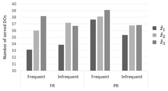
Figure 9.
Average number of served DO per objective with respect to re-optimization frequency and tactic (Frequent—FTR-10 and FTR-20; Infrequent—FTR-40 and FTR-60; FR—full-release tactic; PR—partial-release tactic).
Using objectives that account for vehicle productivity is recommended under operational settings with relatively high vehicle availability, wide TW and especially when the FR tactic is necessary.
6. Concluding Remarks
This paper investigated a new, interesting variant of the dynamic vehicle routing problem with mixed backhauls (DVRPMB), in which the number of vehicles is limited and, thus, not all customer orders may be served within the defined planning horizon. The problem was addressed through periodic re-optimization. For the problem solved in each re-optimization cycle, appropriate objective functions were introduced that account for vehicle productivity. The rationale behind this concept is that anticipating additional work favors reserving fleet capacity for the latter (re-optimization) cycles of the operational horizon, so that newly arriving dynamic orders may be served. Thus, the available fleet should complete as much of the known work as early as possible. To address the m-DVRPMB, a modified branch-and-price algorithm proposed to solve the conventional DVRPMB (with unlimited resources) is proposed.
The experimental investigation focused on answering two key questions: (a) how does the fleet constraint affect the performance of the various re-optimization strategies (combination of re-optimization policy and tactic); and (b) how do the proposed objectives affect overall performance?
Regarding the first question it was illustrated that one should always re-optimize under the PR tactic in as short re-optimization intervals as possible. When using the FR tactic is unavoidable, one should prefer re-optimization over medium intervals.
Regarding the second question, the results indicated that objectives and (which consider vehicle productivity) can yield higher customer service compared to conventional objective . This improvement reaches up to about 15% of more dynamic orders served for cases with wide time-windows or cases for which a majority (more than 50–60%) of dynamic orders may be served by the available fleet. In cases with narrow TW or very limited fleet availability, accounting for vehicle productivity does not seem to help appreciably. Furthermore, with respect to re-optimization strategies (policy and tactic), objectives and perform significantly better than objective under the FR tactic and objective seems to be more efficient for re-optimizing at short re-optimization intervals (i.e., 5–15% of the available working horizon).
In practical applications, such as those that motivated the work in this paper (i.e., courier, e-commerce, money-transfer, etc.), companies are typically aware of their customer demand and size their fleet accordingly, in order to ensure that even on peak demand days a considerable portion (but possibly not all) of the demand that arrives dynamically during the working period can be served. Based on this, the results from this paper indicate that the consideration of vehicle productivity may offer a novel strategy to improve customer service in a straightforward manner. Such strategy seems especially beneficial for applications that operate under the FR policy (i.e., an order that was received and planned during previous re-optimization cycle, cannot be re-scheduled) in order not to cause undue nervousness to the system.
The basic limitation of this work stems from the original decision to solve a dynamic problem through repeated re-optimization; that is through optimizing repeated static snapshots of the state of the dynamic system. This strategy is pseudo-dynamic and may lead to “greediness” and, thus, to suboptimal solutions of the dynamic problem—despite the optimality of the solution of each snapshot. Note that an attempt to address this limitation is through the proposed objective functions that account for vehicle productivity in anticipation of future work. Future work, however, is needed to directly address the intrinsic dynamism of the environment with a true dynamic method.
Another important and relevant consideration in dynamic logistics systems is computational time. Time limitations in practical cases often prohibit extensive optimization and the question arises how to utilize the available time effectively [53]. In general, the increase of memory and CPU time requirements with problem complexity follows a low-power polynomial function when heuristics are employed, rendering the latter more applicable when it comes to dynamic problems. Furthermore, many more recent technologies such as multi-access edge computing, fog computing and cloud computing [54] may be applicable for the solution of dynamic routing optimization problems since they offer powerful computing capabilities. Thus, this may be an interesting area for further study.
The current study may also be extended to investigate the effect of various dispatching policies, i.e., dispatch more vehicles than necessary (or all vehicles available at depot) at the start of operations or during execution (re-optimization), in anticipation of additional work to come. The performance of these dispatching policies may be studied with respect to various factors of the environment (e.g., degree of dynamism, time-window profiles, etc.) or under various re-optimization strategies. Finally, further research may be performed on waiting strategies ([22]) and on how to exploit estimates of future demand provided by stochastic methods ([31]).
Author Contributions
Writing—original draft, G.N.; writingreview & editing, I.M. All authors have read and agreed to the published version of the manuscript.
Funding
This research received no external funding.
Conflicts of Interest
The authors declare no conflict of interests.
Appendix A. Constraints of the Pricing Sub-Problem (SP) in m-DVRPMB
As discussed before, the BP approach proposed defines and solves independent sub-problems (SP), one for each vehicle en route (that will generate new columns ) and only one for the vehicles located at the depot (that will generate columns ). This Appendix describes the constraints involved during the solution of each SP, hence the vehicle index was dropped for simplicity.
As mentioned before, let denote the modified cost associated with arc , given by . Based on this, we modify appropriately the objective function (13) given in Section 4.1 as in Equation (A1) below:
where denotes a decision variable that is equal to if order is served during time interval , where ( denoting the current re-optimization cycle) and 0 otherwise. Profit is calculated according to Section 3.2 (depending on the objective). The constraints of the pricing sub-problem (SP) in m-DVRPMB are given below. It should be noted that variables do not participate in the solution under objective , since in this case :
Constraints (A2) to (A4) ensure that each route starts at the source point and ends at the depot, always preserving the flow along the arcs of the route (where represents the source point of the route and the depot). Constraints (A5) and (A6) ensure that the capacity of the vehicle assigned to the route is not exceeded, where provides the load of a vehicle immediately after serving node , the demand/supply of each order and the maximum capacity of the vehicle. constraints (A7) and (A8) ensure that every customer will be served within its time window, where denote the start of service for order , the correspond to the customer’s time window and is the service time of order . Constraint (A9) ensures that variable will be equal to 1 if customer is served within re-optimization cycle , , where when objective is employed and when objective is used ( is a large positive number). Constraints (A10) ensure that each order will be served only once during the entire remaining horizon. Finally, constraints (A11)–(A12) force variables and flow variables respectively, to assume binary values.
References
- Ninikas, G.; Minis, I. Reoptimization strategies for a dynamic vehicle routing problem with mixed backhauls. Networks 2014, 64, 214–231. [Google Scholar] [CrossRef]
- Ninikas, G.; Minis, I. Load transfer operations for a dynamic vehicle routing problem with mixed backhauls. J. Veh. Routing Algorithms 2018, 1, 47–68. [Google Scholar] [CrossRef]
- Süral, H.; Bookbinder, J.H. The single-vehicle routing problem with unrestricted backhauls. Networks 2003, 41, 127–136. [Google Scholar] [CrossRef]
- Gribkovskaia, I.; Halskau, Ø.; Laporte, G.; Vlcek, M. General solutions to the single vehicle routing problem with pick-ups and deliveries. Eur. J. Oper. Res. 2007, 180, 568–584. [Google Scholar] [CrossRef]
- Gutiérrez-Jarpa, G.; Desaulniers, G.; Laporte, G.; Marianov, V. A branch-and-price algorithm for the Vehicle Routing Problem with Deliveries, Selective Pickups and Time Windows. Eur. J. Oper. Res. 2010, 206, 341–349. [Google Scholar] [CrossRef]
- Desaulniers, G.; Desrosiers, J.; Erdmann, A.; Solomon, M.M.; Soumis, M. The VRP with pickup and delivery. In The Vehicle Routing Problem; Toth, P., Vigo, D., Eds.; Society of Industrial and Applied Mathematics: Philadelphia, PA, USA, 2002. [Google Scholar]
- Berbeglia, G.; Cordeau, J.-F.; Gribkovskaia, I.; Laporte, G. Static pick-up and delivery problems: A classification scheme and survey. Top 2007, 15, 1–31. [Google Scholar] [CrossRef]
- Berbeglia, G.; Cordeau, J.-F.; Laporte, G. Dynamic pick-up and delivery problems. Eur. J. Oper. Res. 2010, 202, 8–15. [Google Scholar] [CrossRef]
- Parragh, S.; Doerner, K.; Hartl, R. A survey on pick-up and delivery problems. Part I: Transportation between customers and depot. J. Betr. 2008, 58, 21–51. [Google Scholar]
- Parragh, S.; Doerner, K.; Hartl, R. A survey on pick-up and delivery problems. Part II: Transportation between pick-up and delivery locations. J. Betr. 2008, 58, 81–117. [Google Scholar]
- Miller, C.E.; Tucker, A.W.; Zemlin, R.A. Integer programming formulations and travelling salesman problems. J. Assoc. Comput. Mach. 1960, 7, 326–329. [Google Scholar] [CrossRef]
- Gutiérrez-Jarpa, G.; Marianov, V.; Obreque, C. A single vehicle routing problem with fixed distribution and optional collections. IIE Trans. 2009, 41, 1067–1079. [Google Scholar] [CrossRef]
- Privé, J.; Renaud, J.; Boctor, F.F.; Laporte, G. Solving a vehicle routing problem arising in soft-drink distribution. J. Oper. Res. Soc. 2006, 57, 1045–1052. [Google Scholar] [CrossRef]
- Aas, B.; Gribkovskaia, I.; Halskau, Ø.; Shlopak, A. Routing of supply vessels to petroleum installations. Int. J. Phys. Distrib. Logist. Manag. 2007, 37, 164–179. [Google Scholar] [CrossRef]
- Gribkovskaia, I.; Laporte, G.; Shyshou, A. The single vehicle routing problem with deliveries and selective pick-ups. Comput. Oper. Res. 2008, 35, 2908–2924. [Google Scholar] [CrossRef]
- Psaraftis, H.N. Dynamic vehicle routing problems. In Vehicle Routing: Methods and Studies; Golden, B.L., Assad, A.A., Eds.; Elsevier Science Publishers B.V.: Amsterdam, The Netherlands, 1988; pp. 223–248. [Google Scholar]
- Schyns, M. An ant colony system for responsive dynamic vehicle routing. Eur. J. Oper. Res. 2015, 245, 704–718. [Google Scholar] [CrossRef]
- Karami, F.; Vancroonenburg, W.; Vanden Berghe, G. A periodic optimization approach to dynamic pickup and delivery problems with time windows. J. Sched. 2020. [Google Scholar] [CrossRef]
- Chen, Z.L.; Xu, H. Dynamic column generation for dynamic vehicle routing with time windows. Transp. Sci. 2006, 40, 74–88. [Google Scholar] [CrossRef]
- Kilby, P.; Prosser, P.; Shaw, P. Dynamic VRPs: A Study of Scenarios; Technical Report APES-06-1998; School of Computer Science, University of St. Andrews: St. Andrews, Scotland, 1998. [Google Scholar]
- Pureza, V.; Laporte, G. Waiting and buffering strategies for the dynamic pickup and delivery problem with time windows. Inf. Inf. Syst. Oper. Res. 2008, 46, 165–175. [Google Scholar] [CrossRef]
- Mitrovic-Minic, S.; Laporte, G. Waiting strategies for the dynamic pickup and delivery problem with time windows. Transp. Res. Part B 2004, 38, 635–655. [Google Scholar] [CrossRef]
- Shieh, H.M.; May, M.D. On-line vehicle routing with time windows, optimization-based heuristics approach for freight demands requested in real-time. Transp. Res. Rec. 1998, 1617, 171–178. [Google Scholar] [CrossRef]
- Larsen, A.; Madsen, O.B.G.; Solomon, M.M. The a-priori dynamic travelling salesman problem with time windows. Transp. Sci. 2004, 38, 459–572. [Google Scholar] [CrossRef]
- Gendreau, M.; Guertin, F.; Potvin, J.Y.; Taillard, É. Parallel tabu search for real-time vehicle routing and dispatching. Transp. Sci. 1999, 33, 381–390. [Google Scholar] [CrossRef]
- Montemanni, R.; Gambardella, L.M.; Rizzoli, A.E.; Donati, A.V. Ant colony system for a dynamic vehicle routing problem. J. Comb. Optim. 2005, 10, 327–343. [Google Scholar] [CrossRef]
- Ichoua, S.; Gendreau, M.; Potvin, J.Y. Diversion issues in real-time vehicle dispatching. Transp. Sci. 2000, 34, 426–438. [Google Scholar] [CrossRef]
- Branke, J.; Middendorf, M.; Noeth, M.; Dessouky, M. Waiting Strategies for Dynamic Vehicle Routing. Transp. Sci. 2005, 29, 298–312. [Google Scholar] [CrossRef]
- Ghiani, G.; Guerriero, F.; Laporte, G.; Musmanno, R. Real-time vehicle routing: Solution concepts, algorithms and parallel computing strategies. Eur. J. Oper. Res. 2003, 151, 1–11. [Google Scholar] [CrossRef]
- Zeimpekis, V.; Tarantilis, C.D.; Giaglis, G.M.; Minis, I. Dynamic Fleet Management: Concepts, Systems, Algorithms & Case Studies; Operations Research/Computer Science Interfaces Series; Springer: Berlin/Heidelberg, Germany, 2007; Volume 38. [Google Scholar]
- Ichoua, S.; Gendreau, M.; Potvin, J.-Y. Exploiting knowledge about future demands for real-time vehicle dispatching. Transp. Sci. 2006, 40, 211–225. [Google Scholar] [CrossRef]
- Goel, A. Fleet Telematics: Real-Time Management and Planning of Commercial Vehicle Operations; Operations Research/Computer Science Interfaces Series; Springer: Berlin/Heidelberg, Germany, 2008. [Google Scholar]
- Larsen, A.; Madsen, O.B.G.; Solomon, M.M. Recent developments in dynamic vehicle routing systems. In The Vehicle Routing Problem: Latest Advances and New Challenges; Operations Research/Computer Science Interfaces; Springer: Berlin/Heidelberg, Germany, 2008; Volume 43, pp. 199–218. [Google Scholar]
- Pillac, V.; Gendreau, M.; Guéret, C.; Medaglia, A.L. A review of dynamic vehicle routing problems. Eur. J. Oper. Res. 2013, 225, 1–11. [Google Scholar] [CrossRef]
- Psaraftis, H.N.; Wen, M.; Kontovas, C.A. Dynamic Vehicle Routing Problems: Three Decades and Counting. Networks 2016, 67, 3–31. [Google Scholar] [CrossRef]
- Máhr, T.; Srour, J.; de Weerdt, M.; Zuidwijk, R. Can agents measure up? A comparative study of an agent-based and on-line optimization approach for a drayage problem with uncertainty. Transp. Res. Part C Emerg. Technol. 2010, 18, 99–119. [Google Scholar] [CrossRef]
- Bent, R.W.; Van Hentenryck, P. Scenario-based planning for partially dynamic vehicle routing with stochastic customers. Oper. Res. 2004, 52, 977–987. [Google Scholar] [CrossRef]
- Goodson, J.C.; Ohlman, J.W.; Thomas, B.W. Cyclic-order neighborhoods with application to the vehicle routing problem with stochastic demand. Eur. J. Oper. Res. 2014, 217, 312–323. [Google Scholar] [CrossRef]
- Ninikas, G. Solving the Dynamic Vehicle Routing Problem with Mixed Backhauls Through re-Optimization. Ph.D. Thesis, University of the Aegean, Chios, Greece, December 2014. [Google Scholar]
- Barnhart, C.; Johnson, E.L.; Nemhauser, G.L.; Savelsbergh, M.W.P.; Vance, P.H. Branch-and-price: Column generation for solving huge integer programs. Oper. Res. 1998, 46, 316–329. [Google Scholar] [CrossRef]
- Desaulniers, G.; Desrosiers, J.; Ioachim, I.; Solomon, M.M.; Soumis, F.; Villeneuve, D. A unified framework for deterministic time constrained vehicle routing and crew scheduling problems. In Fleet Management and Logistics; Crainic, T., Laporte, G., Eds.; Kluwer Academic Publisher: Boston, London, 1998; pp. 57–93. [Google Scholar]
- Desrosiers, J.; Lübbecke, M. A primer in column generation. In Column Generation; Desaulniers, G., Desrosiers, J., Solomon, M.M., Eds.; Springer: New York, NY, USA, 2005; pp. 1–32. [Google Scholar]
- Desaulniers, G.; Desrosiers, J.; Solomon, M.M. Column Generation, No 5. In GERAD 25th Anniversary; Springer: Berlin/Heidelberg, Germany, 2005. [Google Scholar]
- Feillet, D.; Dejax, P.; Gendreau, M.; Gueguen, C. An exact algorithm for the elementary shortest path problem with resource constraints: Application to some vehicle routing problems. Networks 2004, 44, 216–229. [Google Scholar] [CrossRef]
- Feillet, D.; Gendreau, M.; Rousseau, L.M. New Refinements for the Solution of Vehicle Routing Problems with Branch and Price; Technical Report C7PQMR PO2005-08-X; Center for Reasearch on Transportation: Montreal, QC, Canada, 2005. [Google Scholar]
- Savelsbergh, M.W.P.; Sol, M. DRIVE: Dynamic routing of independent vehicles. Oper. Res. 1998, 46, 474–490. [Google Scholar] [CrossRef]
- Desrochers, M.; Desrosiers, J.; Solomon, M. A new optimization algorithm for the vehicle routing problem with time windows. Oper. Res. 1992, 40, 342–354. [Google Scholar] [CrossRef]
- Solomon, M.M. Algorithms for the vehicle routing and scheduling problems with time window constraints. Oper. Res. 1987, 35, 254–265. [Google Scholar] [CrossRef]
- Christofides, N.; Mingozzi, A.; Toth, P. The vehicle routing problem. In Combinatorial Optimization; Christofides, N., Mingozzi, A., Toth, P., Sandi, C., Eds.; John Wiley: Hoboken, NJ, USA, 1979; pp. 315–339. [Google Scholar]
- Clarke, G.; Wright, J. Scheduling of vehicles from a central depot to a number of delivery points. Oper. Res. 1964, 12, 568–581. [Google Scholar] [CrossRef]
- Osman, I.H.; Wassan, N.A. A reactive tabu search meta-heuristic for the vehicle routing problem with back-hauls. J. Sched. 2002, 5, 263–285. [Google Scholar] [CrossRef]
- Mitrovic-Minic, S.; Krishnamurti, R.; Laporte, G. Double-horizon based heuristics for the dynamic pick-up and delivery problem with time windows. Transp. Res. Part B 2004, 38, 669–685. [Google Scholar] [CrossRef]
- Ulmer, M.W. Anticipation versus reactive reoptimization for dynamic vehicle routing with stochastic requests. Networks 2018, 73, 277–291. [Google Scholar] [CrossRef]
- Lee, J.; Kim, D.; Lee, J. Zone-based multi-access edge computing scheme for user device mobility management. Appl. Sci. 2019, 9, 2308. [Google Scholar] [CrossRef]


© 2020 by the authors. Licensee MDPI, Basel, Switzerland. This article is an open access article distributed under the terms and conditions of the Creative Commons Attribution (CC BY) license (http://creativecommons.org/licenses/by/4.0/).