
Analysis of Gradient Vanishing of RNNs and Performance Comparison


Department of Statistical Data Science, ICT Convergence Engineering, Anyang University, Anyang 14028, Korea
Information 2021, 12(11), 442; https://doi.org/10.3390/info12110442
Submission received: 12 August 2021
/
Revised: 19 October 2021
/
Accepted: 22 October 2021
/
Published: 25 October 2021
(This article belongs to the Section Artificial Intelligence)
Abstract
:A recurrent neural network (RNN) combines variable-length input data with a hidden state that depends on previous time steps to generate output data. RNNs have been widely used in time-series data analysis, and various RNN algorithms have been proposed, such as the standard RNN, long short-term memory (LSTM), and gated recurrent units (GRUs). In particular, it has been experimentally proven that LSTM and GRU have higher validation accuracy and prediction accuracy than the standard RNN. The learning ability is a measure of the effectiveness of gradient of error information that would be backpropagated. This study provided a theoretical and experimental basis for the result that LSTM and GRU have more efficient gradient descent than the standard RNN by analyzing and experimenting the gradient vanishing of the standard RNN, LSTM, and GRU. As a result, LSTM and GRU are robust to the degradation of gradient descent even when LSTM and GRU learn long-range input data, which means that the learning ability of LSTM and GRU is greater than standard RNN when learning long-range input data. Therefore, LSTM and GRU have higher validation accuracy and prediction accuracy than the standard RNN. In addition, it was verified whether the experimental results of river-level prediction models, solar power generation prediction models, and speech signal models using the standard RNN, LSTM, and GRUs are consistent with the analysis results of gradient vanishing.
1. Introduction
A recurrent neural network (RNN) is a neural network model proposed in the 1980s [1,2,3] for modeling time series. An RNN is a neural network that combines variable-length input data with a hidden state that depends on previous time steps to produce output data. Through the connections among hidden units associated with the time delay, the model can retain information about the past, enabling it to discover temporal correlations between events that are far away from each other in the data. Although the main purpose of RNNs is to learn long-term dependencies, theoretical and empirical evidence shows that learning to store information for quite long is difficult. To address this problem, one solution is to augment a network with an explicit memory. The first proposal of this type is using long short-term memory (LSTM) networks with special hidden units, the natural behavior of which is to remember inputs for a long time. A special unit called a memory cell acts similar to an accumulator or gated leaky neuron: it has a connection to itself at the next time step that has a weight of 1, so it copies its own real-valued state and accumulates the external signal; however, this self-connection is multiplicatively gated by another unit that learns to decide when to clear the content of the memory [4]. A gated recurrent unit (GRU) was proposed by Cho et al. [5] to make each recurrent unit adaptively capture the dependencies of differences of different time scales. Similar to the LSTM unit, a GRU has gating units that modulate the flow of information inside the unit, without having separate memory cells [6].
RNNs have been widely used in time-series data analysis. In particular, the standard RNN and LSTM have been successfully applied to river-level prediction models [7,8], solar power generation prediction models [9,10], fine-dust prediction models [11,12], energy demand prediction models [13], session-based recommendation models [14,15], stock market index prediction models [16,17], and speech signal models [6].
However, although LSTM and GRUs have been experimentally proven for having higher validation accuracy and prediction accuracy than the standard RNN for long-range dependent input and output data by effectively solving the gradient vanishing problem [6,7,9], research on the theoretical basis has not been conducted thus far. Furthermore, Bengio [18] and Pascanu et al. [19] mathematically proved that training RNNs for long-range dependent input data is difficult due to the gradient vanishing problem because exponentially decreases to 0 over time, where St is the hidden state of the system at time t. Therefore, this study provides a theoretical and experimental basis for the result that LSTM and GRU have more efficient gradient descent than the standard RNN by analyzing and experimenting the gradient vanishing of the standard RNN, LSTM, and GRU. As a result, LSTM and GRU are robust to the degradation of gradient descent even when LSTM and GRU learn long-range input data. This result explains for the experimental previous result that LSTM and GRU have higher validation accuracy and prediction accuracy than the standard RNN.
2. Previous Works
Various RNN algorithms, such as the standard RNN, LSTM, and GRUs, have been proposed. The standard RNN has difficulty in learning long-range dependent input and output data because the backpropagation algorithm does not work effectively due to the gradient vanishing problem as the input data become longer. To overcome this, Hochreiter and Schmidhuber [20] devised LSTM, which has been widely applied to time-series data analysis [6,7,8,9,10,11,12,13,16,17]. Experimental results have proven that LSTM and GRUs have higher validation accuracy and prediction accuracy than the standard RNN by effectively overcoming the gradient vanishing problem through effective learning, even for long-range dependent input and output data [6,7,9].
On the other hand, several studies have been conducted to improve the training speed of RNNs [21,22]. Shi et al. [21] proposed a sentence-independent subsampling stochastic gradient descent algorithm (SIS-SGD) for recurrent neural network-based language models (RNNLM). In SIS-SGD, RNNLM is trained in parallel under the condition of sentence independence. In SIS-SGD, each slave trains a replica of the model on its own training data subset, which is generated by subsampling instead of disjoint partitioning. The experimental results showed that using a multi-thread technique, SIS-SGD can achieve a three-fold speed-up without losing word error rate performance. Khomenko et al. [22] proposed a sequence bucketing algorithm to accelerate RNN mini-batch training for big amount of data. Sequence bucketing algorithm improves training speed by clustering input sequences with large variation into buckets by their length, thus finding a compromise between data structuring and shuffling. In terms of the wall clock time, the system without bucketing (purely random split of sequences on mini-batches) has the longest epoch time (4 h per epoch). The epoch time reduces as the bucket number Q increases. For the value of Q = 3, the best acceleration with minimum validation loss was achieved and the speed up factor is close to 4.
Tran and Song [7] used the standard RNN and LSTM to learn river-level observation data and predict the possibility of flooding and experimentally proved that LSTM has a higher performance than the standard RNN with an accuracy higher than 0.98. Kim et al. [9] compared prediction errors using the standard RNN, LSTM, and GRU for solar power generation prediction models and experimentally proved that the prediction errors of LSTM and GRU were lower than that of the standard RNN. Chung et al. [6] used the standard RNN, LSTM, and GRU for speech signal models and experimentally demonstrated that GRU had a faster convergence speed in learning and a higher prediction accuracy than the standard RNN and LSTM. Bengio [18] and Pascanu et al. [19] mathematically proved that training RNNs for long-range dependent input data is difficult due to the gradient vanishing problem because exponentially decreases to 0 over time, where St is the hidden state of the system at time t.
Therefore, this study aims to provide a theoretical and experimental basis for the result that LSTM and GRU have more efficient gradient descent than the standard RNN by analyzing and experimenting the gradient vanishing of the standard RNN, LSTM, and GRU.
3. Research Results
3.1. Analysis of Gradient Vanishing
To theoretically analyze the performance of the standard RNN, LSTM, and GRU according to their architectures, this study analyzed and compared gradient vanishing among the three models. The standard RNN model is illustrated in Figure 1.
The state St of the hidden layer at time t and the output yt of the output layer at time t can be modeled as follows [4]:
where the activation function σ represents a sigmoid function and U, V, and W are the weight matrices of the network. The weighted parameters of U, V, and W are randomly initialized and learned using the backpropagation algorithm with the stochastic gradient descent.
A standard RNN calculates the sum of weights of input signals simply by receiving the hidden state of the previous time step. However, LSTM delivers the memory cell and hidden state according to the time step, as shown in Figure 2. Hence, it has the advantage of solving the long-range dependence problem.
The output ht, output gate , memory cell , new memory content , forget gate , and input gate in Figure 2 are modeled as follows [6]:
A GRU was proposed by Cho et al. [5] to reflect the dependencies of data along the time axis. As shown in Figure 3, the GRU does not have the memory cell of LSTM. However, it solves the long-range dependence problem by reflecting the information of previous time steps in the output . Because the GRU has one less gate than LSTM, it has fewer network parameters than LSTM. The GRU can be modeled as follows [6]:
Experimental results have proven that LSTM and GRU have higher validation accuracy and prediction accuracy than the standard RNN [6,7,9], but a theoretical basis has not been presented. This study attempts to show that the experimental results of [6,7,9] were derived because LSTM and GRU have more efficient gradient descent than the standard RNN and they are robust to the degradation of gradient descent even when learning long-range input data.
For learning in RNNs, let us assume that the output at time is , and the actual observed data are represented by .
If the loss function is defined as the mean square error of and , , then the backpropagation algorithm is applied from the right side of the computed graph of the unfolded network to calculate the gradient of for every state. This condition is used to update weights to minimize . Because is a function that can be differentiated with respect to , the gradient of can be expressed as a gradient for every state of . Therefore, the gradient vanishing of RNN is caused by the gradient vanishing for all states of .
In the standard RNN, if , then the gradient for the initially hidden state of the output at time can be expressed by the chain rule as follows:
Therefore, decreases to as increases, and the gradient vanishing problem is generated.
In LSTM, the gradient for the initial memory cell state of the output at time can be expressed by the chain rule as follows:
However, because
and
If Equation (7) is substituted in Equation (6), then it is expressed as follows:
Therefore, if are repetitively substituted in Equation (6), then remains in , and does not decrease to even if increases. Moreover, if at the output gate , then and . Because includes and does not decrease to , does not decrease to even if increases. Therefore, does not decrease to even if increases. The gradient for the initial hidden state of output can be expressed by the chain rule as follows:
However,
and
Therefore, when are substituted repeatedly in Equation (9), then does not decrease to even if increases because remains in . Moreover, and . Because includes and does not decrease to , does not decrease to even if increases. Hence, does not decrease to even if increases. In LSTM, the initial memory cell state is preserved because the memory cell is delivered along the time axis. Therefore, the LSTM can effectively learn long-range dependent input data because the possibility that the LSTM can effectively overcome the gradient vanishing problem increases as compared to the standard RNN.
In the GRU, the gradient for the initially hidden state of output at time can be expressed by the chain rule as follows:
However, because
Using Equation (11), can be expressed as:
Therefore, when are repeatedly substituted in Equation (11), contains , which does not decrease to even if increases in the case that each element of in Equation (3) does not converge to when increases. The case where each element of can converge to when increases is the case where the input data stream is a constant data stream. Furthermore, because the update gate , candidate activation , and reset gate all include , even if increases, the gradient for of , the gradient for of , and the gradient for of do not decrease to 0 in the case that each element of in Equation (3) does not converge to when increases. Therefore, because the initial hidden state is preserved by reflecting the information from previous time steps by the output in the GRU, the possibility that the GRU can effectively learn long-range dependent input data increases as compared to the standard RNN.
3.2. Numerical Example
In this Section we provided experimental results that LSTM and GRU have more efficient gradient descent than the standard RNN by experimenting the gradient vanishing of the standard RNN, LSTM, and GRU. As a result, LSTM and GRU are robust to the degradation of gradient descent even when LSTM and GRU learn long-range input data, which means that the learning ability of LSTM and GRU is greater than standard RNN when learning long-range input data.
The dataset used in the experiment is the Jena Climate Dataset. The Jena Climate Dataset is a weather timeseries dataset recorded at the weather station of the Max Planck Institute for Biogeochemistry in Jena, Germany. The Jena Climate Dataset is made up of 14 different quantities (such air temperature, atmospheric pressure, humidity, wind direction, etc.) that were recorded every 10 min, from 1 January 2009 to 31 December 2016. The sample rate was set to 6, and an hour data was modified as single input data. We trained the standard RNN, LSTM, and GRU to predict data after 12 h by using the data from the previous 120 h as a training data.
Figure 4 shows the changes of the derivatives in the Equation (4), in the Equation (6), in the Equation (9), in the Equation (11) over time (hour), respectively. Figure 5 shows the changes of the derivatives in the Equation (4), in the Equation (6), in the Equation (9), in the Equation (11) over time (epoch), respectively. The values of the four gradients are very small, so the absolute values of the gradients are expressed in log-scale. The time axis represents the hour in Figure 4 and the epoch in Figure 5, respectively. As shown in Figure 4, the absolute values of the derivatives in the Equation (11) for the GRU converges with the largest value, the absolute values of the derivatives in the Equation (6) for the LSTM converges with the second value, and the absolute values of the derivatives in the Equation (4) for the standard RNN converges with the third value, and the absolute values of the derivatives in the Equation (9) for the LSTM converges with the smallest value. The absolute value of the derivatives of the output of the GRU with respect to the initial value and the absolute value of the derivatives of the memory cell state of the LSTM with respect to the initial value , converge with larger value than the absolute value of the derivatives of with respect to the initial value . The experimental result shows the validity of the analysis result in Section 3.1.
As shown in Figure 5, the absolute values of the derivatives in the Equation (6) for the LSTM converges with the largest value, the absolute values of the derivatives in the Equation (9) for the LSTM converges with the second value, and the absolute values of the derivatives in the Equation (11) for the GRU converges with the third value, and the absolute values of the derivatives in the Equation (4) for the standard RNN converges with the smallest value. The absolute value of the derivatives of the memory cell state of the LSTM with respect to the initial value , the absolute value of the derivatives of the memory cell state of the LSTM with respect to the initial value , and the absolute value of the derivatives of the output of the LSTM with respect to the initial value converge with larger value than the absolute value of the derivatives of with respect to the initial value . The experimental result also shows the validity of the analysis result in Section 3.1.
4. Discussion of Other Works
In this section, the experimental results of [6,7,9] are shown and compared with the gradient vanishing analysis results presented in Section 3. Tran and Song [7] predicted the water level of the Trinity River (Texas, USA) using the standard RNN, RNN-backpropagation through time (BPTT), and LSTM models. The input data were the river flow rate, precipitation, and water level recorded every 15 min from 2013 to 2015. The prediction results generated through the model consisted of river levels after 30 and 60 min. The data evaluated here were the data from 2016. The verification errors and prediction errors were measured using the root mean square error (RMSE). The experimental results of [7] are shown in Table 1 and Figure 6.
As shown in Table 1 and Figure 6, the validation error of LSTM was 0.0045, lower than 0.0076 for the standard RNN. The prediction error of LSTM was also lower in the prediction of water level at 30 min later and 60 min later.
To predict solar power generation, Kim et al. [9] defined five datasets and predicted power generation using the standard RNN, LSTM, and GRU models. The solar power generation prediction results were the output for input data from at least one hour before until three days later. In addition, the prediction error was measured using the mean square error (MSE). The prediction error measurement result for dataset 1 (the input data are composed of the photovoltaic power generation) is shown in Figure 7. In LSTM, learning converges first for input data up to 24 h before, and the MSE was the smallest at 0.0024.
In the case of dataset 2 (input data consist of photovoltaic power generation, solar irradiance, and temperatures), the error measurement result is shown in Figure 8. The RNN model converged for input data from 9 h before, LSTM converged for input data from 24 h before, and the GRU converged for the input data from 21 h before. LSTM and GRU also showed the lowest prediction error (MSE) at 0.0022.
In [6], the prediction accuracy was compared by measuring the learning convergence speeds of the standard RNN, LSTM, and GRU models for the MuseData dataset and by measuring the negative log-likelihood of the sequence prediction probability. The convergence speed and prediction accuracy of the three models are shown in Figure 9 and Figure 10. As shown in these figures, the GRU showed the highest learning convergence speed and prediction accuracy.
The experimental results of [6,7,9] are consistent with the findings presented in Section 3, where LSTM and GRU show higher validation accuracy and prediction accuracy than the standard RNN because they can effectively learn long-range dependent input data owing to robustness to the degradation of gradient descent. However, it is not easy to make an absolute comparison of the two models, and their performances vary by the type of input data.
5. Conclusions
This study is meaningful in that it derived a basis for the difference in the validation accuracy and prediction accuracy among the three representative RNN models (i.e., standard RNN, LSTM, and GRU models) by analyzing and experimenting their gradient vanishing.
The standard RNN model can be expressed as Equation (1). If the hidden state of the system is and the output is at time , then can be expressed as Equation (4). Hence, the gradient vanishing problem is generated if decreases to .
In the case of LSTM, the gradient for the initial memory cell state of output at time can be calculated by Equation (5), and in this equation includes . Similarly, can be calculated using Equation (8), and in this equation includes . The two terms do not decrease to 0 even if increases. Hence, the LSTM is more robust to degradation of gradient than the standard RNN.
In the case of the GRU, the gradient for the initial hidden state of output at time can be expressed as Equation (11), and in this equation includes . Because this term does not decrease to 0 even if increases, the GRU is more robust to degradation of gradient than the standard RNN.
The numerical example presented in Section 3.2 shows that the gradients of the LSTM and the GRU converge over time with relatively larger values than the standard RNN. The experimental result shows the validity of the analysis results in Section 3.1.
As shown in Table 1 and Figure 6 derived from [7] and Figure 7 derived from [9], the validation error and prediction error of LSTM are lower than those of the standard RNN. As shown in Figure 7 derived from [9], the prediction error of the GRU is lower than that of the standard RNN. In addition, Figure 9 and Figure 10 derived from [6] show that the GRU has a faster convergence speed and a higher prediction accuracy than those of the standard RNN and LSTM. However, the prediction accuracies of the GRU and LSTM vary by data type. The experimental results examined in Section 4 confirm that the gradient vanishing analysis results of this study can explain the experimental results of [6,7,9].
Funding
This research received no external funding.
Conflicts of Interest
The author declares no conflict of interest.
References
- Rumelhart, D.E.; Hinton, G.E.; Williams, R.J. Learning representations by back-propagating errors. Nature 1986, 323, 533–536. [Google Scholar] [CrossRef]
- Elman, J. Finding structure in time. Cogn. Sci. 1990, 14, 179–211. [Google Scholar] [CrossRef]
- Werbos, P.J. Generalization of backpropagation with application to a recurrent gas market model. Neural Netw. 1988, 1, 339–356. [Google Scholar] [CrossRef] [Green Version]
- LeCun, Y.; Bengio, Y.; Hinton, G. Deep learning. Nature 2015, 521, 436–444. [Google Scholar] [CrossRef] [PubMed]
- Cho, K.; Merrienboer, B.; Gulcehre, C.; Bahdanau, D.; Bougares, F.; Schwenk, H.; Bengio, Y. Learning phrase representations using RNN encoder-decoder for statistical machine translation. In Proceedings of the Empirical Methods in Natural Language Processing (EMNLP), Doha, Qatar, 25–29 October 2014. [Google Scholar]
- Chung, J.; Gulcehre, C.; Cho, K.H.; Bengio, Y. Empirical evaluation of gated recurrent neural networks on sequence modeling. arXiv 2014, arXiv:1412.3555. [Google Scholar]
- Tran, Q.K.; Song, S. Water level forecasting based on deep learning: A use case of Trinity River-Texas-The United States. J. KIISE 2020, 44, 607–612. [Google Scholar] [CrossRef]
- Cho, W.; Kang, D. Estimation method of river water level using LSTM. In Proceedings of the Korea Conference on Software Engineering, Busan, Korea, 20–22 December 2017; pp. 439–441. [Google Scholar]
- Kim, H.; Tak, H.; Cho, H. Design of photovoltaic power generation prediction model with recurrent neural network. J. KIISE 2019, 46, 506–514. [Google Scholar] [CrossRef]
- Son, H.; Kim, S.; Jang, Y. LSTM-based 24-h solar power forecasting model using weather forecast data. KIISE Trans. Comput. Pract. 2020, 26, 435–441. [Google Scholar] [CrossRef]
- Yi, H.; Bui, K.N.; Seon, C.N. A deep learning LSTM framework for urban traffic flow and fine dust prediction. J. KIISE 2020, 47, 292–297. [Google Scholar] [CrossRef]
- Jo, S.; Jeong, M.; Lee, J.; Oh, I.; Han, Y. Analysis of correlation of wind direction/speed and particulate matter (PM10) and prediction of particulate matter using LSTM. In Proceedings of the Korea Computer Congress, Busan, Korea, 2–4 July 2020; pp. 1649–1651. [Google Scholar]
- Munir, M.S.; Abedin, S.F.; Alam, G.R.; Kim, D.H.; Hong, C.S. RNN based energy demand prediction for smart-home in smart-grid framework. In Proceedings of the Korea Conference on Software Engineering, Busan, Korea, 20–22 December 2017; pp. 437–439. [Google Scholar]
- Hidasi, B.; Karatzoglou, A.; Baltrumas, L.; Tikk, D. Session-based recommendations with recurrent neural networks. In Proceedings of the International Conference on Learning Representations (ICLR), San Juan, Puerto Rico, 2–4 May 2016. [Google Scholar]
- Wu, S.; Ren, W.; Yu, C.; Chen, G.; Zhang, D.; Zhu, J. Personal recommendation using deep recurrent neural networks in NetEase. In Proceedings of the IEEE International Conference on Data Engineering (ICDE), Helsinki, Finland, 16–20 May 2016. [Google Scholar]
- Kwon, D.; Kwon, S.; Byun, J.; Kim, M. Forecasting KOSPI Index with LSTM deep learning model using COVID-19 data. In Proceedings of the Korea Conference on Software Engineering, Seoul, Korea, 5–11 October 2020; Volume 270, pp. 1367–1369. [Google Scholar]
- Fischer, T.; Krauss, C. Deep learning with long short-term memory networks for financial market predictions. Eur. J. Oper. Res. 2018, 270, 654–669. [Google Scholar] [CrossRef] [Green Version]
- Bengio, Y.; Simard, P.; Frasconi, P. Learning long-term dependencies with gradient descent is difficult. IEEE Trans. Neural Netw. 1994, 5, 157–166. [Google Scholar] [CrossRef] [PubMed]
- Pascanu, R.; Mikolov, T.; Bengio, Y. On the difficulty of training recurrent neural networks. In Proceedings of the International Conference on Machine Learning (PMLR), Atlanta, GA, USA, 17–19 June 2013. [Google Scholar]
- Hochreiter, S.; Schmidhuber, J. Long short-term memory. Neural Comput. 1997, 9, 1735–1780. [Google Scholar] [CrossRef] [PubMed]
- Shi, Y.; Hwang, M.-Y.; Yao, K.; Larson, M. Speed up of recurrent neural network language models with sentence independent subsampling stochastic gradient descent. In Proceedings of the INTERSPEECH, Lyon, France, 25–29 August 2013; pp. 1203–1207. [Google Scholar]
- Khomenko, V.; Shyshkov, O.; Radyvonenko, O.; Bokhan, K. Accelerating recurrent neural network training using sequence bucketing and multi-GPU data parallelization. In Proceedings of the IEEE Conference on Data Stream Mining & Processing (DSMP), Lviv, Ukraine, 23–27 August 2016; pp. 100–103. [Google Scholar]
Figure 1.
Standard RNN model (Source: [4]).
Figure 1.
Standard RNN model (Source: [4]).

Figure 2.
LSTM model.
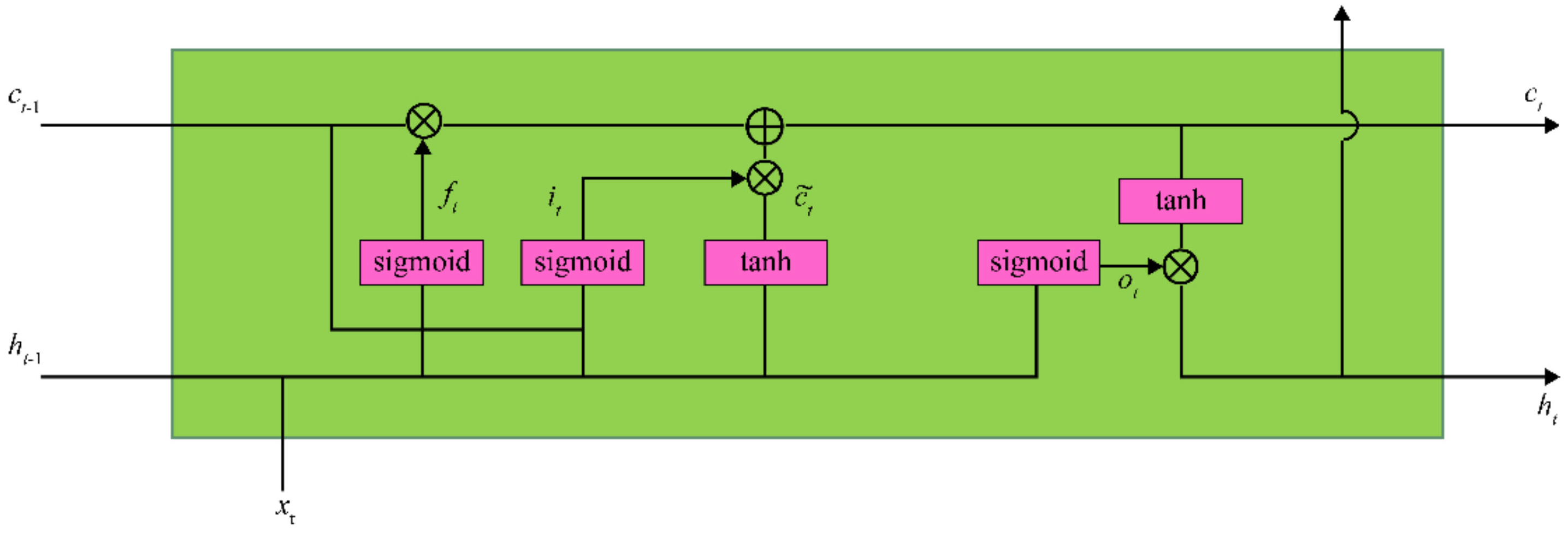
Figure 3.
GRU model.
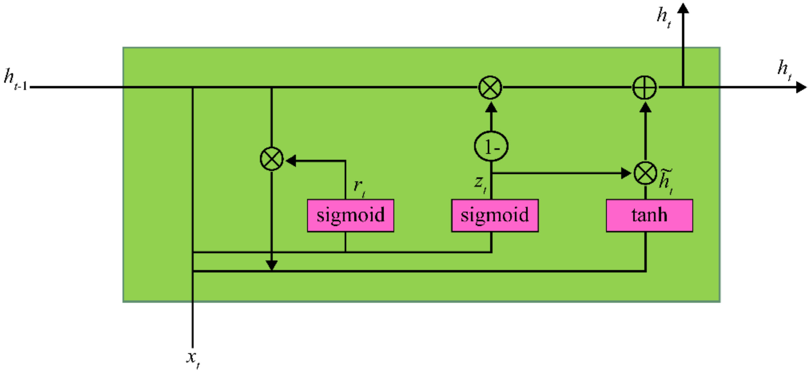
Figure 4.
Changes of the derivatives of the three models over time (hour).
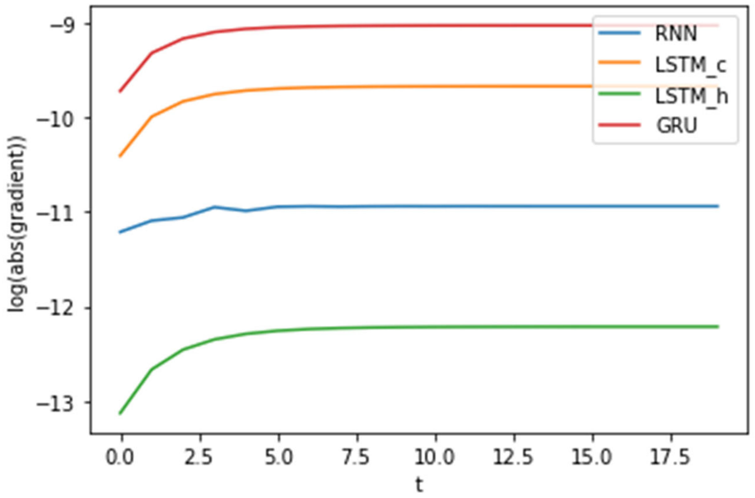
Figure 5.
Changes of the derivatives of the three models over epoch.
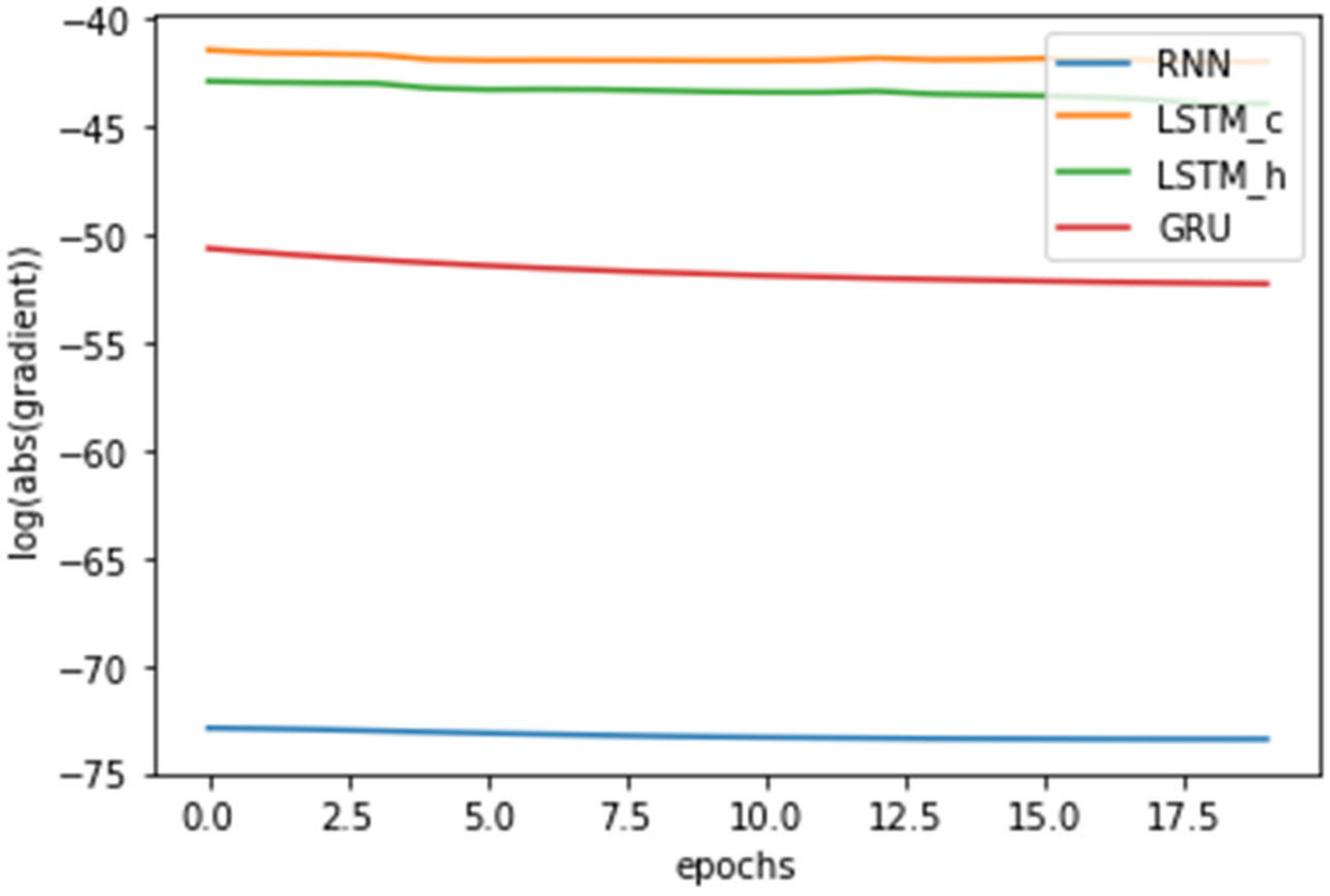
Figure 6.
Convergence process of the three algorithms (after the fifth epoch) (Source: [7]).
Figure 6.
Convergence process of the three algorithms (after the fifth epoch) (Source: [7]).
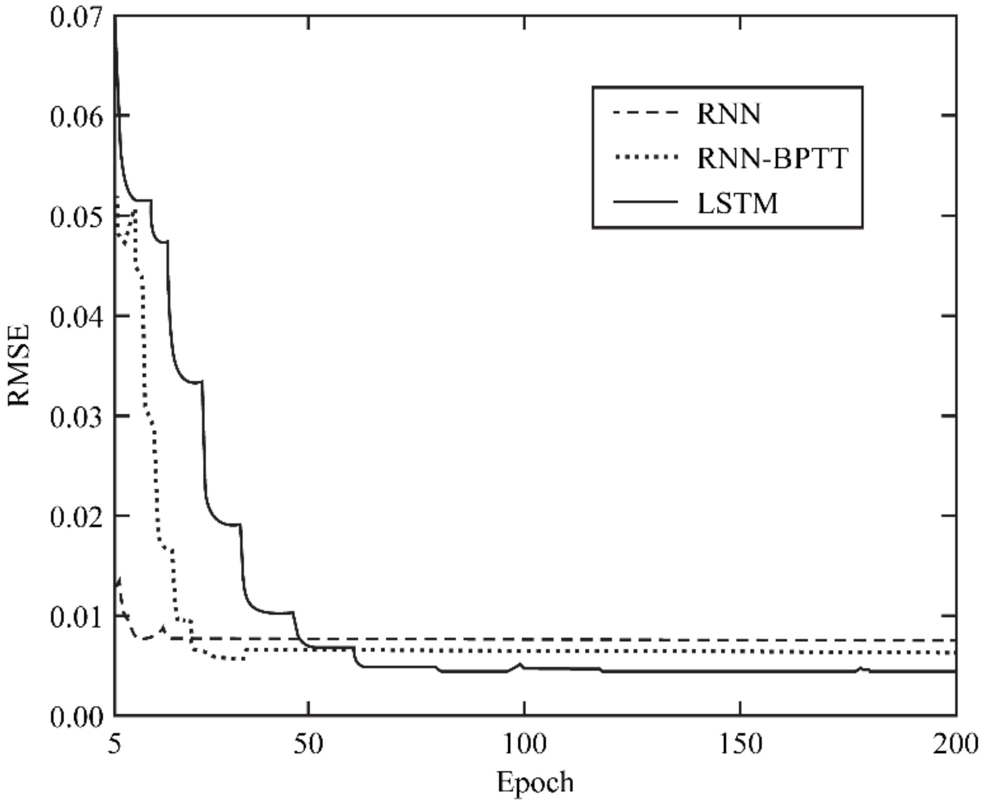
Figure 7.
MSE curve according to the past data length of dataset 1. LSTM converges from 24 h, whereas the RNN and GRU converge thereafter. The error rate at LSTM with 24 h past data is the lowest at 0.0024 (Source: [9]).
Figure 7.
MSE curve according to the past data length of dataset 1. LSTM converges from 24 h, whereas the RNN and GRU converge thereafter. The error rate at LSTM with 24 h past data is the lowest at 0.0024 (Source: [9]).
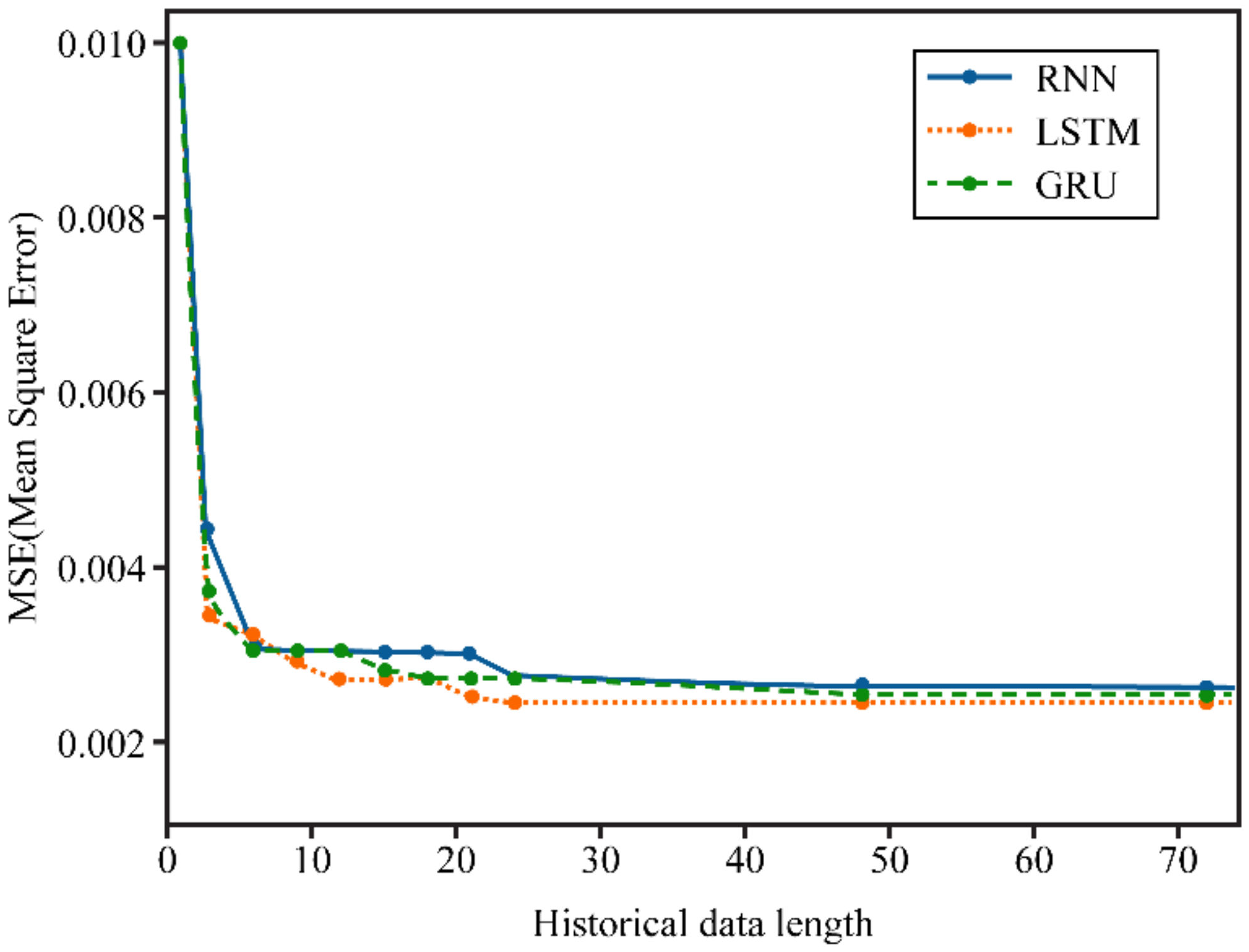
Figure 8.
MSE curve according to the past data length of dataset 2. The RNN converges from 9 h, LSTM converges from 24 h, and the GRU converges from 21 h. The error rate at LSTM with 24 h past data and GRU with 21 h past data are the lowest at 0.0022 (Source: [9]).
Figure 8.
MSE curve according to the past data length of dataset 2. The RNN converges from 9 h, LSTM converges from 24 h, and the GRU converges from 21 h. The error rate at LSTM with 24 h past data and GRU with 21 h past data are the lowest at 0.0022 (Source: [9]).
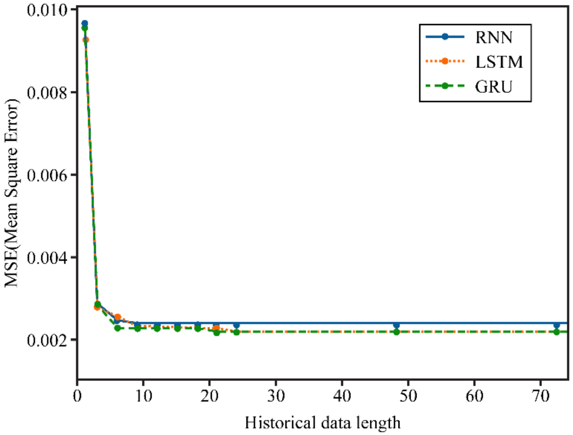
Figure 9.
Learning curves for the training and validation sets of different types of units with respect to the number of iterations. The x-axis corresponds to the number of epochs, and the y-axis corresponds to the negative log likelihood of the learning probability distribution over sequences in the log scale (Source: [6]).
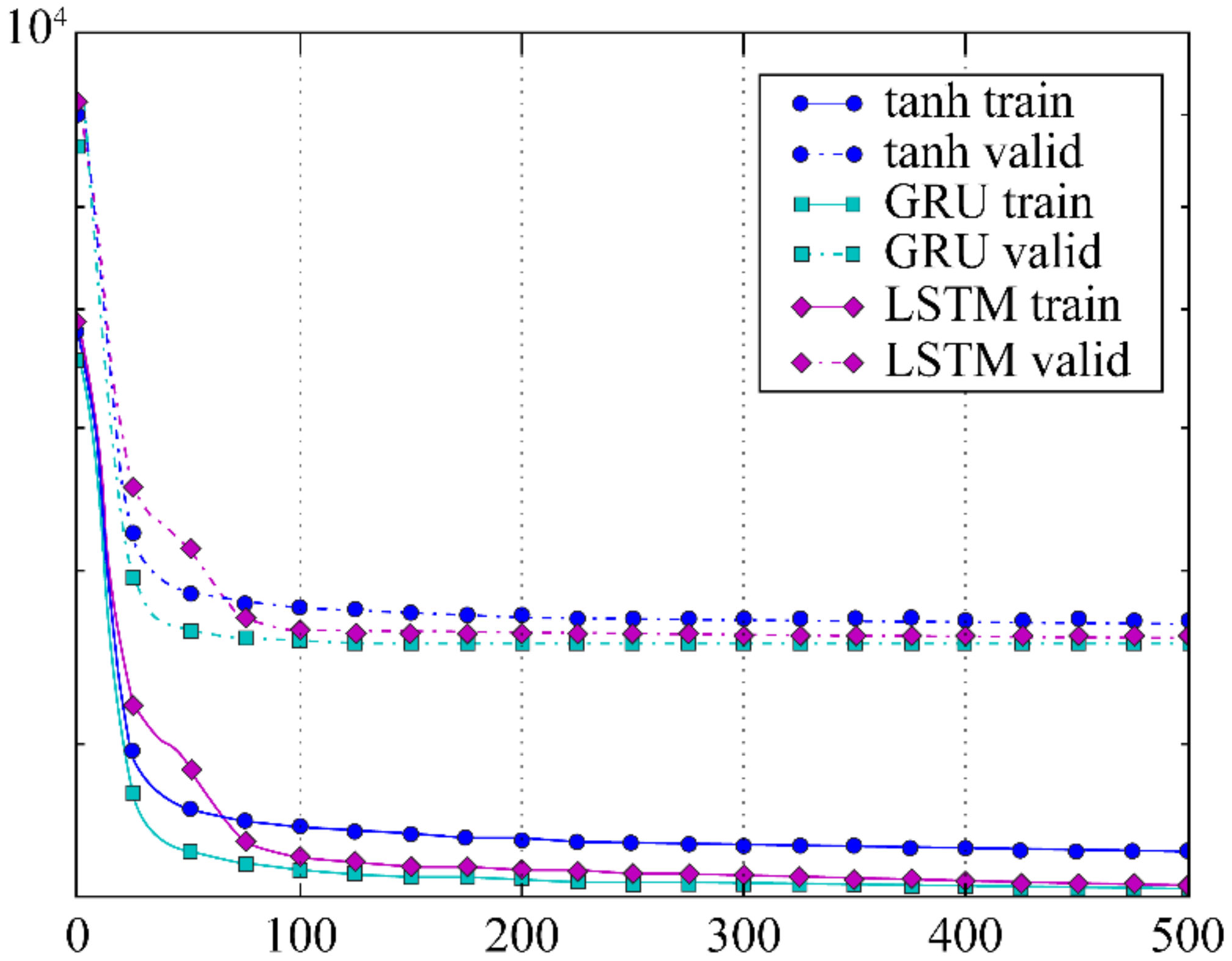
Figure 10.
Learning curves for the training and validation sets of different types of units with respect to the wall clock time (seconds). The x-axis corresponds to the wall clock time (seconds) and the y-axis corresponds to the negative log likelihood of learning probability distribution over sequences in the log scale (Source: [6]).


Table 1.
Validation errors and prediction errors of the standard RNN, RNN-BPTT, and LSTM (Source: [7]).
Table 1.
Validation errors and prediction errors of the standard RNN, RNN-BPTT, and LSTM (Source: [7]).
| Standard RNN | RNN-BPTT | LSTM | ||
|---|---|---|---|---|
| Training | Training time (hours) | ~14 | ~22 | ~67 |
| Validation (RMSE) | 0.0076 | 0.0064 | 0.0045 | |
| Testing | One prediction (milliseconds) | ~1.6 | ~1.6 | ~2.8 |
| RMSE (30 min) | 0.0102 | 0.0091 | 0.0077 | |
| RMSE (60 min) | 0.0105 | 0.0092 | 0.0079 |
Publisher’s Note: MDPI stays neutral with regard to jurisdictional claims in published maps and institutional affiliations. |
© 2021 by the author. Licensee MDPI, Basel, Switzerland. This article is an open access article distributed under the terms and conditions of the Creative Commons Attribution (CC BY) license (https://creativecommons.org/licenses/by/4.0/).
Share and Cite
MDPI and ACS Style
Noh, S.-H. Analysis of Gradient Vanishing of RNNs and Performance Comparison. Information 2021, 12, 442. https://doi.org/10.3390/info12110442
AMA Style
Noh S-H. Analysis of Gradient Vanishing of RNNs and Performance Comparison. Information. 2021; 12(11):442. https://doi.org/10.3390/info12110442
Chicago/Turabian StyleNoh, Seol-Hyun. 2021. "Analysis of Gradient Vanishing of RNNs and Performance Comparison" Information 12, no. 11: 442. https://doi.org/10.3390/info12110442
Note that from the first issue of 2016, this journal uses article numbers instead of page numbers. See further details here.