Help Me Learn! Architecture and Strategies to Combine Recommendations and Active Learning in Manufacturing

Abstract

This research work describes an architecture for building a system that guides a user from a forecast generated by a machine learning model through a sequence of decision-making steps. The system is demonstrated in a manufacturing demand forecasting use case and can be extended to other domains. In addition, the system provides the means for knowledge acquisition by gathering data from users. Finally, it implements an active learning component and compares multiple strategies to recommend media news to the user. We compare such strategies through a set of experiments to understand how they balance learning and provide accurate media news recommendations to the user. The media news aims to provide additional context to demand forecasts and enhance judgment on decision-making.

1. Introduction

The decreased cost of sensors and connectivity [1], along with the development of the Internet of Things, Cloud Computing, Big Data Analytics and Blockchain technologies [2] have enabled an increasing digitalization of manufacturing and the introduction of new paradigms, such as Cyber-Physical Systems (CPS) [3,4] and Digital Twins (DTs) [5,6,7]. Moreover, they bring extensive added value to Industry 4.0 [8], enabling more effective operations, cost saving, and better product quality [9].

While an explosive growth of data available in the manufacturing industry has been observed [10], captured through sensors or made available from software, such as Enterprise Resource Planning (ERP) or Manufacturing Execution Systems (MES), much collective, semantic, and tacit knowledge that the employees are aware of is not digitalized. Furthermore, much of the digitalized data are not labeled, and thus no supervised learning algorithms can be applied to it. It is thus essential to identify how informative the newly collected data instances are to make good decisions regarding data management and machine learning models.

Much of the missing information can be introduced into the digital domain by asking users specific questions. Users can be queried regarding missing labels, asked for feedback on particular entries, or missing domain knowledge. The collection of locally observed collective knowledge can be achieved through a specialized solution [11,12]. The particular case of querying a user for labels given a large pool of unlabeled data is addressed by a sub-field of machine learning known as Active learning (AL) [13]. Active learning attempts to identify the most informative data instances, which are presented to the oracle (e.g., a human expert) asking for a label, reducing the data annotation effort. Newly labeled data are incorporated into the existing dataset and can be fed to the machine learning models. Batch machine learning models require regular deployments to make available the last trained version to the manufacturing software.

Active learning reduces the labeling stress posed on the user and provides a solution to the users’ reticence to provide information and feedback [14]. Though, active learning alone does not solve the data labeling issue: a good user experience is key to the success of such a system [15], impacting conversion rates (amount of labeled samples) and user satisfaction (users will not abandon the feature or application) [16]. Therefore, we designed a user interface considering users’ feedback can be implicit [17] or explicit. Assuming that the quality of our entries is acceptable (implicit feedback, if no other feedback is provided), we provide means to the user to signal disagreement (explicit feedback) [18,19,20]. When providing recommendations to the users, candidate data instances identified by an active learning strategy do not guarantee their quality and the consequent good user experience [21]. A compromise is required to balance exploration and exploitation while delivering good results. Furthermore, we ranked the unlabeled data entries to ensure entries whose high-quality is most probable are displayed first, and those that do not meet a certain quality threshold are not shown at all. For particular cases, such as when collecting feedback on decision-making options suggested to the user, we allowed the user to provide their own input. This way, we gather additional domain knowledge when the options provided so far do not satisfy the user. New domain knowledge provided by the users can be later incorporated into the application, promoting continuous knowledge gathering and learning.

This paper evolves previous work done in [22]. The scientific contributions of this paper are twofold. First, it describes an architecture we developed to realize a system that combines semantic technologies, machine learning, and explainable artificial intelligence to provide forecasts, explanations, and contextual information while guiding users’ decision-making. Second, it compares nine active learning scenarios to understand the learning versus recommendation trade-off. Then, we evaluate them implementing a prototype application and recommending four categories of media news that enhance planners’ awareness in a demand forecasting setting. In addition, we describe the implementation of a knowledge-based decision-making options recommender system implemented to advise logisticians regarding transport scheduling based on demand forecasts.

The media news we recommend to the users relates to four aspects influencing the demand for automotive engine components produced by a European original equipment manufacturer selling its products worldwide. First, the demand forecasting models were trained using real-world data provided by manufacturing partners of the European Horizon 2020 project FACTLOG [23,24,25]. Data we used included three years of shipment information daily, a month of demand forecasts for material and clients at a daily level, feature relevance for every prediction, forecast explanations created based on those feature rankings, and decision-making options created based on demand forecasts and heuristics.

We evaluate the outcomes of the machine learning models across different active learning scenarios assessing two metrics: area under the receiver operating characteristic curve (ROC AUC) [26] and Mean Average Precision (MAP) [27]. ROC AUC is widely adopted as a classification metric due to its desirable properties, such as being threshold independent and invariant to a priori class probabilities. We measure ROC AUC considering prediction scores cut at a threshold of 0.5. On the other side, MAP is a popular metric in the information retrieval domain, computing the precision of the recommendation set with the size associated with the relevant item’s rank. Both metrics are used to assess the performance of recommender systems [28].

The rest of this paper is structured as follows: Section 2 presents related work, and Section 3 details the architecture we designed to satisfy the requirements described above. Section 4 describes the demand forecasting use case we considered to build and test the concept architecture and system. Section 5 presents the user interface, describing each of the components we built into it. Section 6 describes the decision-making recommender system implementations, while Section 7 details the experiments and results obtained when applying active learning for media news categorization and recommendation. Finally, Section 8 provides the conclusions and outlines future work.

2. Related Work

In this section, we first briefly introduce scientific literature describing demand forecasting models related to the automotive industry. We then describe related work regarding Explainable Artificial Intelligence (XAI), and conclude with an overview of scientific works related to the active learning field.

2.1. Demand Forecasting

Products’ demand forecasting requires the application of different approaches conditioned by the demand characteristics. Widely adopted criteria to characterize the demand relate to the demands’ lead times variance [29], the average demand interval magnitude [30], or the coefficient of variation (see Equation (1)) [31].

$$CV=\frac{\mathit{Demand}\mathit{Standard}\mathit{Deviation}}{\mathit{Demand}\mathit{Mean}}.$$

(1)

Demand is closely related to the product’s characteristics and is influenced by the economic context, market type, and customer expectations. Among factors affecting the demand in the automotive industry we find personal income [32], fuel prices [33,34], gross domestic product [35], inflation and unemployment rates [36,37]. This information can be collected and encoded to datasets used to train machine learning models, which learn to predict future demand based on past data.

Statistical and machine learning models were successfully applied to provide accurate car, and car components demand forecasts. Among the most frequent machine learning algorithms used to train the models we find the Support Vector Machine (SVM) [36], Multiple Linear Regressor (MLR) [38,39] and Artificial Neural Networks (ANN) [40,41,42]. Popular statistical forecasting methods include the autoregressive integrated moving average (ARIMA) [32,43], autoregressive moving average (ARMA) [33] and moving average models [44].

While the accuracy of the demand forecasting models is critical for their adoption, given the influence on decision-making, it is imperative to provide details on the rationale followed by the model. Such insights help the user understand the reasons behind the forecast and decide whether it can trust it or not [25]. Furthermore, it has been argued that including domain context can further aid the planners assess the forecasts’ soundness, and eventually correct it before making a decision [45,46,47].

2.2. Explainable Artificial Intelligence

While the Industry 4.0 paradigm represents a great potential for the manufacturing industry [48], risks associated with its implementation, such as the complexity of integration or the perceived risks of novel technologies [49] must be mitigated. One such perceived risk is the difficulty of providing an intelligible explanation regarding the machine learning models’ predictions. Usual reasons behind models’ opaqueness are: (i) the complexity of the formal structure of the model, which can be beyond human comprehension [50], or alien to human reasoning; and (ii) intentional hiding of the inner workings of the model (e.g., to avoid exposing some trade secret, or sensitive information) [51]. Research on how to provide intelligibility on the reasons behind the forecast and transparency regarding the machine learning forecasting model is known as explainable artificial intelligence [46]. Such insights and explanations increase the trust in AI models and provide additional information to assist users’ decision-making.

Best practices on how to convey the insights regarding the models’ reasoning process require the explanation to resemble a logic explanation [52], and take into account relevant context. Among context elements, ref. [53] considers three related to the explainee: (i) the user profile to whom the explanation is given; (ii) the goal of the explanation; and (iii) if the explanation is either global (describes the average AI model forecast), or local (describes a specific forecast instance). Common explanation types include feature rankings, prototype (local) explanations, and counterfactual explanations. Multiple techniques were developed to compute feature rankings, which convey information on which features exercised most influence on a given forecast (local explanation) [54,55,56], or forecasts in general (global explanation). Prototype explanations are data instances obtained from the train set, which are similar to the feature vector used to issue the prediction [57]. Such samples help us to understand which instances most likely influenced the model learning to provide a particular forecast. Finally, counterfactual explanations provide perturbed data samples that produce a different forecasting outcome than the original data instance [58,59,60]. Such samples allow the user to understand what values need to be changed to change a forecast outcome. Ideally, the perturbed features correspond to actionable aspects, on which the user can be advised to take action to influence future outcomes [61].

In the context of manufacturing, XAI technologies have been tested in several scenarios such as predictive maintenance [62], real-time process management [63], and quality monitoring [64]. One of our research goals is to highlight the models’ explainability in smart manufacturing processes, aligning XAI technologies with human interaction. We also aim to collect feedback on the quality of such explanations since there are few validated measurements for user evaluations on explanations’ quality [65].

2.3. Active Learning

Active learning is a sub-field of machine learning that studies how to improve the learners’ performance by asking questions to an oracle (e.g., a human annotator), under the assumption that unlabeled data are abundant, while the labels are expensive to obtain [13]. Since users are usually reluctant to provide information and feedback, AL can be used to identify a set of data instances on which the users’ input conveys the most valuable information to the system [14]. While active learning in itself helps to reduce the labeling effort focusing on the data that provides new information, it has been demonstrated that explainable artificial intelligence can provide meaningful information to the user, increasing the accuracy of the labels provided [66]. Furthermore, feedback on the explanations can be used to enhance them in the future further. A framework of three components can be used to gather feedback, considering a forecasting engine, an explanation engine, and a feedback loop to learn from the users [67].

The scientific literature describes multiple approaches towards the realization of active learning [13,68,69]. Regarding how the unlabeled data instances are obtained, we distinguish three scenarios: (i) membership query synthesis; (ii) stream-based selective sampling; and (iii) pool-based active learning. Membership query synthesis requires some mechanism (e.g., adversarial generative sampling [70]) to synthesize new data instances for the specific label they were requested. Stream-based selective sampling assumes a stream of unlabeled data instances is available. A decision must be made for each data instance regarding whether it should be discarded or provided to the oracle for labeling. Such a decision can be made based on an informativeness measure or determining a region of uncertainty, querying the data instances within it. Finally, pool-based active learning assumes a pool of unlabeled data from which data instances are selected greedily based on an informativeness measure, which enables to rank the entire pool before selecting the best candidate data instance.

While we envision that active learning can be applied to enhance the explanations provided by XAI, and the decision-making options recommendations we provide to the users regarding manufacturing-related operations [14], in this work, we only compare different active learning strategies to classify and recommend media news to the users. We extend the approach proposed by [67] to collect feedback from forecasts, forecast explanations, media news related to demand forecasting, and decision-making options we recommend to the users. When recommending media news to the users, we evaluate our approaches against baselines described in [21]. Those baselines allow us to understand the exploration and exploitation trade-off required to learn from promising unlabeled data instances while providing good recommendations to the users.

Active Learning for Text Classification

Text classification is a procedure of assigning predefined labels to the text and is considered one of the most fundamental tasks in natural language processing [71]. Most classical machine learning approaches follow the two steps, where in the first step (hand-crafted), features are extracted from the input texts and in the second step, the features are fed to a classifier that makes predictions. The choices of features include the bag-of-words (BoW) approach with various extensions, such as BoW with TF-IDF weighting [72], while the choices of classifiers include logistic regression and support vector machines [73]. In some tasks, such approaches can still provide competitive baselines.

To address the limitations of hand-crafted features, neural approaches have been explored, where the model learns to map the input text to a low-dimensional continuous feature vector [73,74]. Feature extraction from text can be done using the approaches, such as word2vec [75], doc2vec [76], universal sentence encoder [77], or by using transformer-based models, such as BERT [78,79] and RoBERTa [80]. In some approaches, there are multiple ways to obtain a single feature vector for the input text. E.g., this can be done, by using only the vector of a specific word from text, for example the classification token, or by averaging the feature vectors of all the words. Different techniques might yield different performances on a given task [79,81]. A neural feature extractor can be used to produce fixed feature vectors that are fed to the classifier as in the classical two-step approach, or the neural model can be trained end-to-end on the given task.

To achieve a satisfying performance, text classification models need a large number of annotated examples to learn from. As manual labeling is a resource-intensive task, active learning can alleviate some of the efforts. Different feature extraction techniques, classification models and query strategies might be used [74,81,82,83]. The prediction uncertainty-based query strategies are widely adopted and used with both single model or committees [84,85] approaches. We are primarily interested in evaluating the strategies that tackle the trade-off between learning and recommendation, so we follow the conclusions from [81] to select the feature extraction method and classification model.

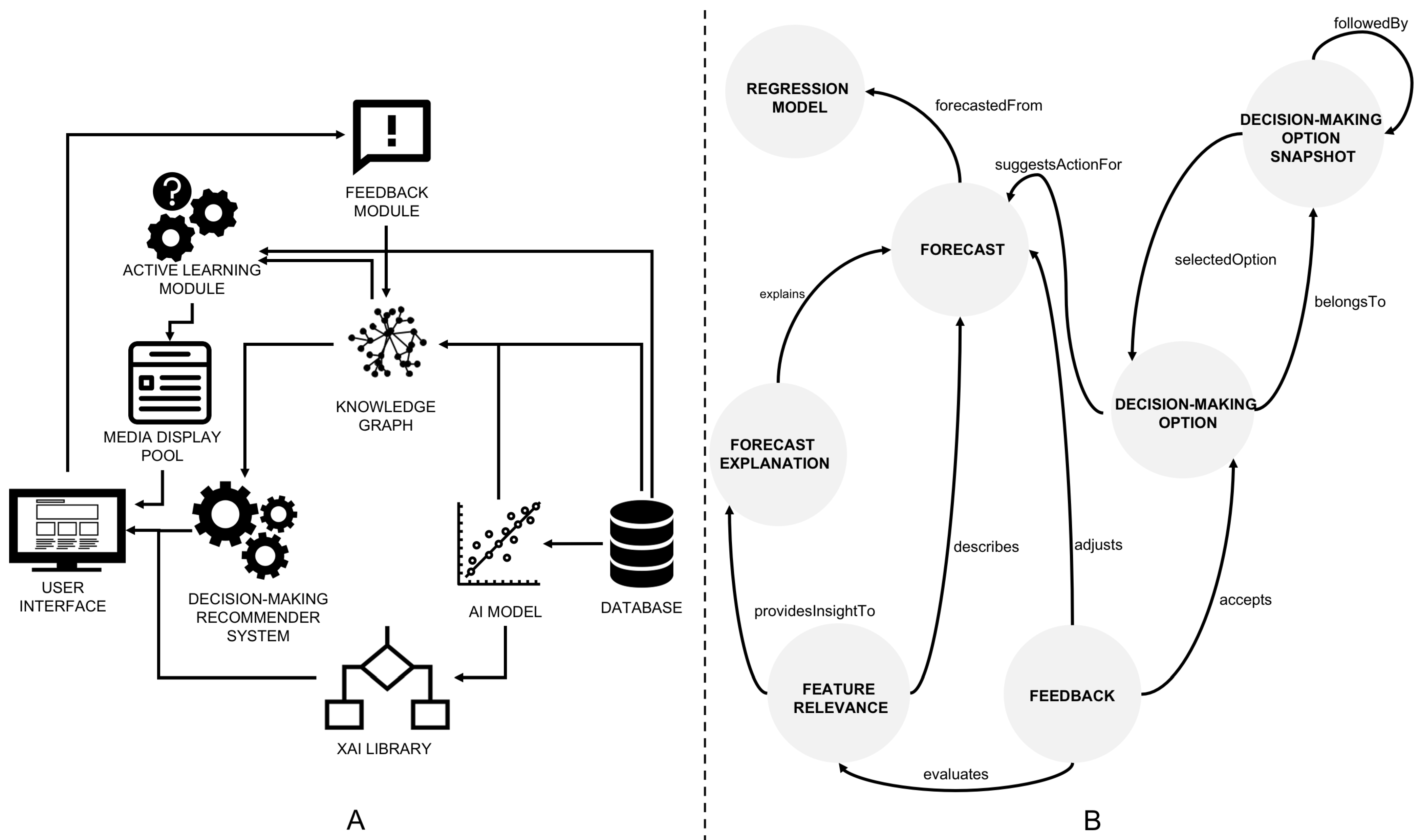
3. Proposed Architecture

To realize the system described in Section 1, we first drafted and iterated an architecture, which requires the following components: (see Figure 1A):

• Database, stores operational data from the manufacturing plant. Data can be obtained from ERP, MES, or other manufacturing platforms;
• Knowledge Graph, stores data ingested from a database or external sources and connects it, providing a semantic meaning. To map data from the database to the knowledge graph, virtual mapping procedures can be used, built considering ontology concepts and their relationships;
• Active Learning Module, aims to select data instances whose labels are expected to be most informative to a machine learning model and thus are expected to contribute most to its performance increase when added to the existing dataset. Obtained labels are persisted to the knowledge graph and database;
• AI model, aims to solve a specific task relevant to the use case, such as classification, regression, clustering, or ranking;
• XAI Library, provides some insight into the AI models’ rationale used to produce the output for the input instance considered at the task at hand. E.g., in the case of a classification task, it may indicate the most relevant features for a given forecast or counterfactual examples;
• Decision-Making Recommender System recommends decision-making options to the users. Recommended decision-making options can vary depending on the users’ profile, specific use case context, and feedback provided in the past;
• Feedback module, collects feedback from the users and persists it into the knowledge graph. The feedback can correspond to predetermined options presented to the users (including labels for a classification problem) or custom feedback written by the users;
• User Interface, provides relevant information to the user through a suitable information medium. The interface must enable user interactions to create two-way communication between the human and the system.

The knowledge graph is a central component of the system. Instantiated from an ontology (see Figure 1B), it relates forecasts, forecast explanations, decision-making options, and feedback provided by the users. To ensure context regarding decision-making options and feedback provided is preserved, different relationships are established. The feedback entity directly relates to a forecast, forecast explanation, and decision-making option. While a chain of decisions can exist for a given forecast, there is a need to model the decision-making options available at each stage and the sequence on which they are displayed. To that end, the decision-making snapshot entity aims to capture a list of decision-making options provided at a given point in time. A relationship between decision-making option snapshots (followedBy) provides information on such a sequence. For each decision-making snapshot, a selectedOption relationship is created to the user’s selected decision-making option. A suggestsActionFor relationship is created between the forecast entity and entities that correspond to the first decision-making options displayed for that particular forecast. Since the decision-making options are linked to decision-making option snapshots and preserve a sequential relationship, all decision-making options can be traced back to the forecast that originated them.

4. Use Case

Demand forecasting is a key component of supply chain management since it directly affects production planning and order fulfillment. Accurate forecasts enable operational and strategic decisions regarding manufacturing and logistics for deliveries. We developed a model to forecast demand on a material and client level daily. The model was trained on three years of data for 516 time-series corresponding to 279 materials and 149 clients of a European automotive original equipment manufacturer’s daily demand. While the forecasts were created and evaluated for all of the clients and materials, we used a subset of them to evaluate the application (e.g., the forecast explanations, media news we display, and recommended decision-making options). We generated forecast explanations using the LIME library [54], but other approaches could be used too (e.g., LionForests [86] or Shapley values [87]). We implemented two strategies for decision-making options recommendations, which allowed us to select a new transport or chose among existing ones. The first one consisted of a set of heuristics that satisfy certain criteria (e.g., have enough capacity to satisfy the expected demand for a given client), while the second one was a knowledge-based recommender. To enhance the context understanding related to demand forecasting, we display media entries for predetermined topics (Automotive Industry, Global Economy, Unemployment, and Logistics) obtained from a media event retrieval system for that day. Media events are queried based on a set of keywords. We developed machine learning models to classify media entries as interesting or not to the users and then gather labels from the users for new media entries. Given there is no need to deliver such media news entries in real-time, we opted to follow a pool-based active learning strategy, persisting all media news event entries, and selecting those considered most informative from the pool of unlabeled data.To provide decision-making options to the users, we implemented two recommender systems: one based on heuristics, and a knowledge-based recommender system. We describe both in Section 6.

5. User Interface

To provide forecasts, forecast explanations, media news, and decision-making options to the user, we developed a user interface with five distinct parts (see Figure 2). Among them we find:

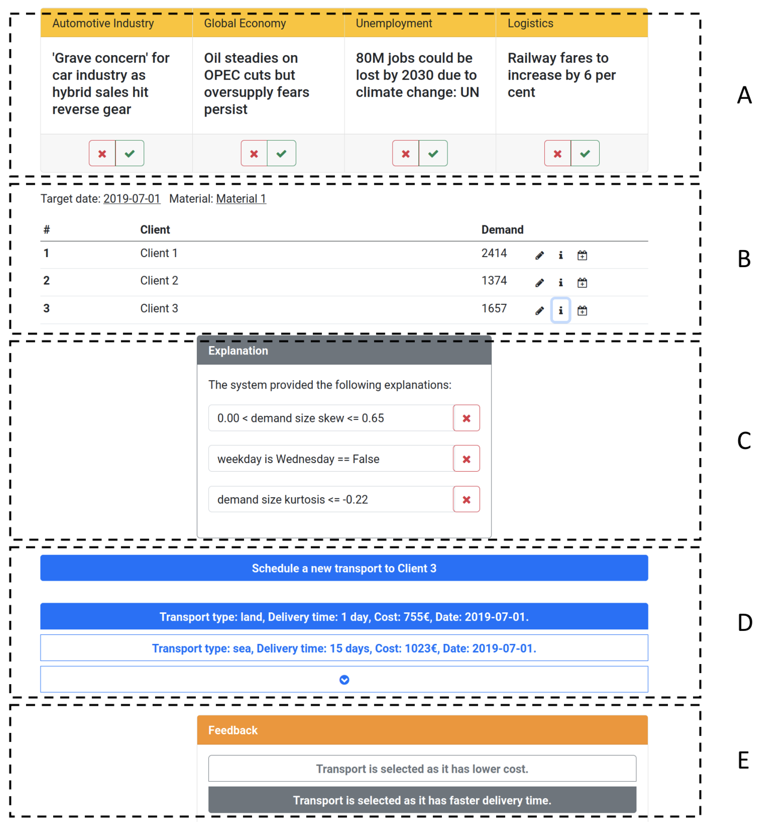
A

Media news panel: displays media news regarding the automotive industry, global economy, unemployment, and logistics. The user can provide explicit feedback on them (if they are suitable or not), acting as an oracle for the active learning classifier. Once feedback is provided, a new piece of news is displayed to the user.

B

Forecast panel: given the date and material, it displays the forecasted demand for different clients. For each forecast, three options are available: edit the forecast (providing explicit feedback on the forecast value), display the forecast explanation, and display the decision-making options. The lack of editing on displayed forecasts is considered implicit feedback approving the forecasted demand quantities.

C

Forecast explanation panel: displays the forecast explanation for a given forecast. Our implementation displays the top three features identified by the LIME algorithm as relevant to the selected forecast. If users consider that some of the displayed features do not explain the given forecast, they can provide feedback by removing it from the list.

D

Decision-making options panel: displays possible decision-making options for a given forecast or step in the decision-making process. In particular, the decision-making options relate to possible shipments. If no good option exists, the user can create its own.

E

Feedback panel: gathers feedback from the user to understand the reasons behind the chosen decision-making option. While some pre-defined are shown to the user, we always include the user’s possibility to add their reasons and enrich the existing knowledge base. Furthermore, such data can be used to expand feedback options displayed to the users in the future.

6. Decision-Making Options Recommendation

Demand forecasts influence decision-making on a wide variety of scenarios: from raw material orders to workers hiring and upskilling to logistics arrangements to meet the required deadlines. Decision-making recommender systems can alleviate such decision-making by suggesting to the user appropriate actions based on the projected demand. In particular, we implemented a decision-making options recommender system considering the logistics use case. We consider two possible scenarios. The first scenario refers to the user who schedules a new transport for a given demand, material, client, and date. Here, the decision-making options are the possible transports, differing in transport type, delivery time, and price. The second possible scenario relates to the user who decides to use an existing transport. Here each decision-making option selects one of the existing transports. In both steps, the recommendation module ranks the decision-making options from most to least relevant.

We developed two recommendation strategies: a heuristic-based and a knowledge-based approach. The heuristic-based recommender system follows simple rules, handcrafted either by the domain expert or simply by the system’s developer based on his incomplete knowledge about the problem. At each step, the user should have the possibility to select any of the possible options regardless of their ranking. Such a system has no learning capacity, and therefore has little potential to improve the users’ experience. The recommendation quality directly depends on the quality of the designed rules. An example of such a heuristic rule is consistently ranking the transports according to the price or keeping only existing transports delivering in the client’s proximity and ranking them according to the remaining capacity.

The knowledge-based approach provides recommendations based on the feature vectors’ similarity to a target vector describing users’ requirements. To that end, each decision-making option at the given step is represented as a vector v. The representation captures all necessary information for the ranking, encoding the context up to the current step, the corresponding decision-making option, and its relation to all other possible decision-making options (the decision-making options snapshot). The model assigns the relevance score to each option based on v. The ranking is determined by sorting the scores from highest to lowest.

The representation and the underlying model should be expressive enough to cover the scenarios encountered in the use case. As with the heuristic-based strategy, domain knowledge heavily influences the design of features, but the content-based strategy provides greater flexibility. The features directly capture the context, which in our use case includes the forecasted demand, date, material, and client; the decision-making option, which in the case of scheduling a new transport includes the transport type, time of delivery, capacity, and price; and the relation of the decision-making option to the whole set of available options to capture, how this option is different from others and why it should be preferred.

Among the constraints of our recommender system, we must mention that we had no data regarding the physical characteristics of each product we created demand forecasts for. In addition, while we had no information regarding the specific addresses of the clients ordering such products, we had information of the destination country. To mitigate these constraints, we collected pricing and delivery time information for air, land, and sea shipments considering single standard forty feet containers from Slovenia to fourteen countries. Such data was retrieved from two specialized web-pages (we collected data regarding pricing and shipment time from World Freight Rates (https://worldfreightrates.com/freight) and SeaRates (https://www.searates.com/freight). We retrieved the data between 12 July and 16 July 2021). Finally, given the application was not deployed to a production environment yet, we lack data regarding logisticians’ interaction and choices, which would enable recommender systems’ performance evaluation. We envision that more complex models can be developed in the future once data regarding users’ interaction with decision-making options is obtained.

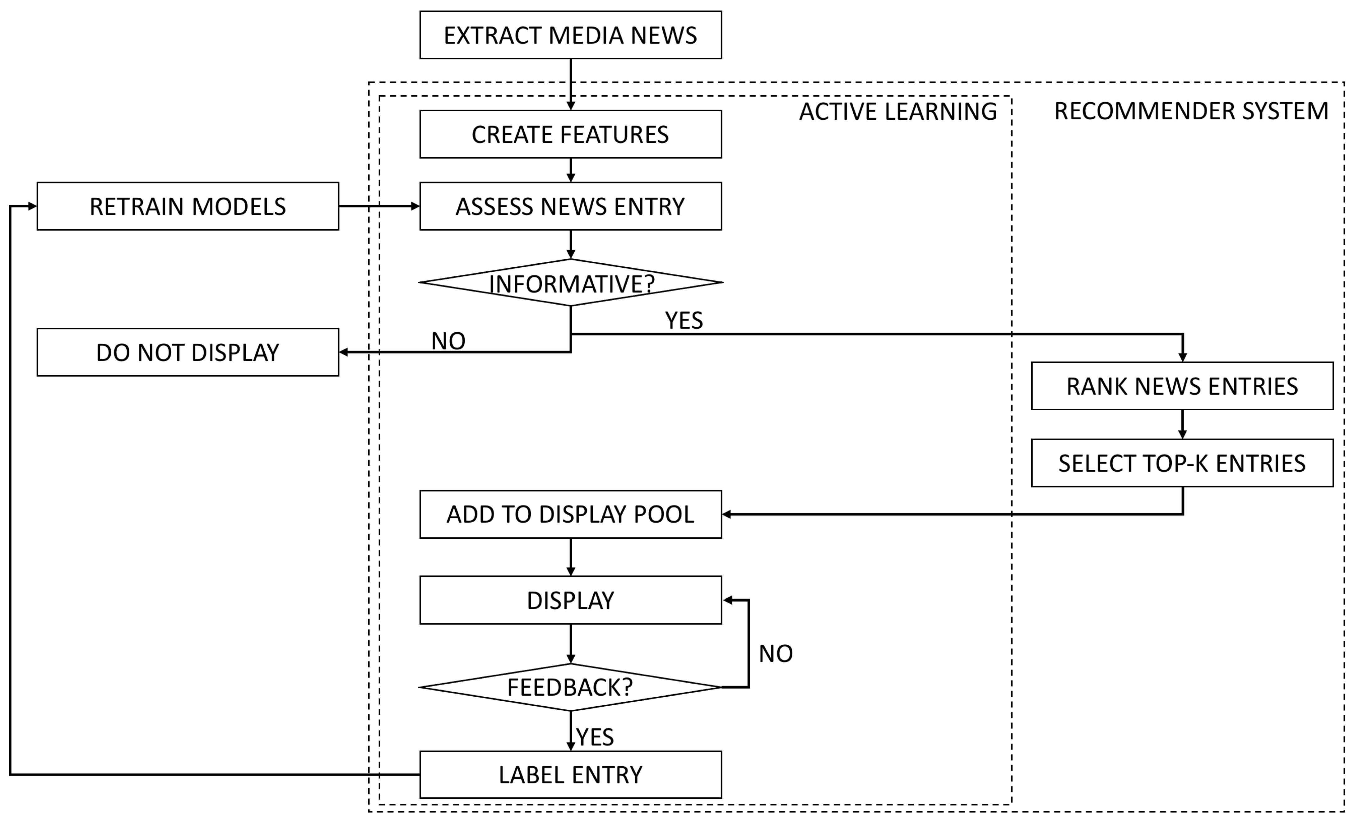
7. Active Learning for Media News Categorization and Recommendation

When providing a demand forecast and the explanation that conveys an intuition regarding the reasons behind the forecast, the user can be interested in getting media news on events that can influence demand. In particular, when forecasting engine parts for the automotive industry, the user can be interested in news regarding the automotive industry, the global economy, unemployment, or logistics. While media news can be retrieved from some news intelligence platforms, keywords based queries can issue many false positives. It is thus imperative to develop a recommender system capable of discriminating and prioritizing good quality news over those considered false positives. Furthermore, it is desired that such a model improve the quality of discrimination over time and require as little manual labeling effort as possible. To realize this, we built a set of active learning binary classifiers, each one informing if the media news considered does fit into a specific media news category or not. We consider the end-user is at the same time the news consumer and the active learning’s oracle, providing feedback regarding unlabeled instances. In our design, we display the news and collect feedback regarding them in the same user interface. This poses an exploration–exploitation dilemma since the same user interface space must be optimized to provide high-quality media news balancing between those entries where high confidence on the category exists but provide little additional information to the existing dataset, and those entries where the confidence is lower, but can provide a higher degree of novelty to the dataset [21]. In particular, each day, at most, ten pieces of news per each of the four categories are displayed to the user. The user can then provide positive or negative feedback (label) regarding each piece of news. The news should be informative for the system as the goal is to achieve good classification performance as soon as possible. On the other hand, the displayed news events should also be relevant so that the system is usable to the users after the first few iterations. The set of displayed news events on each day should therefore balance the learning vs. recommendation (exploration vs. exploitation). In this research, we do not deal with the cold-start problem since we consider it can be mitigated by pre-training the models with a set of manually annotated instances before starting the active learning dynamics. We have evaluated nine strategies (see

Table 1. Active learning and recommendation strategies.

Strategy	Description
Random	Selects the k random instances at each step.
Uncertain	Selects k instances with highest uncertainty score at each step.
Certain	Selects k instances with lowest uncertainty score, that is, most certain examples.
Positive Uncertain	Select at most k instances that were labeled as positive by the classifier and have the highest uncertainty scores.
Positive Certain	Select at most k instances that were labeled as positive by the classifier and have the lowest uncertainty scores.
Positive Certain and Uncertain	Select at most $k/2$ positive points with lowest and at least $k/2$ points with highest uncertainty score.
Alpha Trade-Off $(\alpha =0.5,0.75,1.0)$	We adapt the strategy proposed by [21]

), balancing learning and recommendation.

Different measures can be used to measure the classification certainty of the model, which is needed in the 5 out of 9 strategies presented in the Table 1. We use the uncertainty of classification which is defined for a single sample x as $U\left(x\right)=1-\underset{y}{max}P\left(y\right|x)$ where a higher value of $U\left(x\right)$ means higher uncertainty. In the case of the SVM model, the distance to the separating hyper-plane is an indicator of uncertainty, with the example having the lowest distance being most uncertain [88].

Strategy Uncertain straightly implements the uncertainty assumption that labels of the instances with the highest classification uncertainty are the most informative. It solely focuses on learning as such instances tend not to be the most relevant for the recommendation. The Random strategy is included as a baseline, and so is the Certain strategy, which only selects the least uncertain instances whose labels should provide the most negligible value for the system according to the uncertainty assumption. To also address the recommendation, the Positive uncertain strategy selects the instances labeled as positive by the model as this already signals that the instance is likely to be relevant for the recommendation. At the same time, it might still provide some value for learning due to uncertainty. On the other hand, the Positive certain strategy selects only the positive instances. Therefore, it ranks them according to the certainty, which should highly favor the recommendation while providing little value for learning. The Positive certain and uncertain strategy tries to include both recommendation and learning by following the Positive certain strategy for the first $k/2$ instances (or less if there are not enough positive instances) to provide relevant recommendations and next following the uncertainty strategy to select at least the $k/2$ instances relevant for learning.

The Alpha trade-off strategy is adapted from [21] and has a parameter $\alpha$, used to control between learning and recommendation. It selects the instances according to the formula

$$x_{\alpha }=\underset{x}{arg\; min}|P_{\alpha }-P(y=1|x)|$$

with $P_{\alpha }$ being the ${\left(100\alpha \right)}^{\mathrm{th}}$ percentile of the distribution of predictive probabilities of positive class induced on the pool of new examples. For example $P_{0.5}$ equals to the median probability and $P_{1.0}$ equals to the maximum probability of the positive class assigned to an instance from the pool. According to [21], $\alpha =0.5$ selects the instance with highest uncertainty from the pool and thus favours learning while $\alpha =1.0$ selects most certainly positive instance and thus favours recommendation. Setting $\alpha =0.75$ could therefore provide a trade-off between learning and recommendation. The k instances closest to $P_{\alpha }$ are selected to form the pool.

Positive certain and Alpha trade-off ($\alpha =1.0$) differ by the fact that Positive certain limits only to instances that were labeled as positive and selects at most k instances which have the lowest uncertainty score (highest probability of positive class), while Alpha trade-off ($\alpha =1.0$) always selects k examples according to the decreasing probability of positive class. Similarly as Positive certain, the Positive uncertain strategy also limits to examples that were labeled as positive and selects at most k instances, which have the highest uncertainty score (lowest probability of positive class).

7.1. Active Learning Experiments

The active learning experiments were performed on a dataset of media news events classified into four categories: Automotive Industry, Global Economy, Unemployment, and Logistics. The dataset was manually annotated by three human annotators, based on the specific keywords used in each category to retrieve them (see

Table 2. Active learning dataset categories, keywords used to query them, the number of instances per category, the number of days without entries for a given category, and the median of events per day for that category (MEPD). “# Instances” stands for “the number of instances”.

Category	Keywords	# Instances	Missing Data	MEPD
(A) Automotive Industry	car sales demand, new car sales, vehicle sales, car demand, automotive industry	3865	10 days	20
(B) Global Economy	global GDP projection, global economic outlook, economic forecast	853	29 days	5
(C) Unemployment	unemployment rate, unemployment numbers, unemployment report, employment growth, long-term unemployment	3801	8 days	22
(D) Logistics	logistics, maritime transport, railroad transport, freight, cargo transport, supply chain	28,231	0 days	133

). The media news events were retrieved daily for a period of six months (from July 2019 to December 2019) from Event Registry [89], a well-established media events monitoring platform that has monitored mainstream media since 2014. The first month of the dataset was reserved for training the initial version of the models and for tuning the model’s hyperparameters. The last month of the dataset was reserved for testing the classification performance of the models at each active learning step. The remaining data was used to execute the active learning experiments and evaluate the recommendation performance at each step. We provide an overview regarding the dataset in

Table 3. Overview of the active learning datasets with total number of instances per each split, ratio of negative and positive instances, as labeled by the human annotators, number of iterations on the learning set when AL is used and maximum number of possible queried instances by limiting the budget with $k=10$ instances per iteration. “# instances” denotes “the number of instances”.

	A	B	C	D
Initialization set size (# instances)	607	128	638	4388
Learning set size (# instances)	3070	693	2882	23,051
Test set size (# instances)	795	160	919	5180
Ratio of negative instances (all sets)	69.83%	65.06%	92.50%	97.71%
Ratio of positive instances (all sets)	30.17%	34.94%	7.50%	2.29%
Number of AL iterations	122	115	122	123
Number of possible selected instances (given $k=10$)	1138	644	1132	1205

. We report the dataset size regarding the number of instances per dataset split (initialization set, learning set used with AL, and test set). We can observe that the datasets vary in size, with B being the smallest and D being almost two magnitudes larger than B. Further, we include the ratio of negative and positive instances, as labeled by the human annotators. The datasets are differently balanced, with D being most unbalanced as the ratio of positive instances is only $2.29\%$. We consider that the datasets’ diversity strengthens the experiments designed to evaluate diverse scenarios. In addition to the dataset information, in Table 3 we also report the number of AL iterations per each dataset (the number of days when at least one news event is available) and the maximum number of instances that could be queried for a category, per day, on average. While we conducted the experiments with a fixed budget of at most k data instances per day; note that this number is smaller than k times the number of days; less than k instances were available for some days.

We executed the following procedure (see Figure 3). For each day, we retrieved all available events for that given day, and for each media news entry, we created the corresponding feature vector and assessed whether it should be displayed to the user to gather feedback (label the instance) or not. This decision was made based on a strategy (see Table 1) that considered how informative the news entries were to the existing dataset, and their quality towards the target category, given the requirement that the events should be both relevant for the user (recommendation quality) and informative for the model (improvement of classification). For each day, we selected at most k events, which were then shown to the user. We set $k=10$, based on the median number of events per day, and acknowledging it is a common practice to query a fixed number of instances at each step according to the literature [81]. Once the media entry was displayed to the user, it was incorporated into the existing dataset if it provided an annotation.

There are cases where the model can recommend less than k events. For example, this could be due to not enough events for a particular category exist that day or that only $k^{\prime }<k$ of them are relevant or need a label. Thus, fewer events of that category are displayed to the user.

We use a separate test set to measure the active learning models’ classification performance to evaluate the models. In contrast, the recommendations’ quality is measured at each step of active learning using the gold labels of the displayed news events. To measure the models’ discrimination power, we adopted the ROC AUC, a widely used metric due to its invariance to a priori class probabilities. On the other hand, to measure the quality of the recommendations, we adopted the MAP metric, which computes the precision of the recommendation set, and is not affected by the number of entries considered in each particular case (the desired property when $k^{\prime }<k$ media news events are shown to the user).

Only the titles of news events were considered for classification. We used two groups of classification models, namely, the ones that are retrained on the labeled set on each iteration of AL and the ones that are trained incrementally (online) on each new presented labeled instance. We used logistic regression (LR), support vector machine (SVM), and random forest (RF) in the first group. Among the online algorithms, we trained an SGD-based logistic regression, a perceptron, and a passive-aggressive classifier (PA) [90], obtaining best results with the latest. The selection of the batch models follow the related work [74,81] where the SVM model was identified as a frequent choice for active learning for text classification. The models that are retrained were also selected based on their fast training time.

We experimented with three text representation techniques: TF-IDF weighted BoW representation, which is a classical representation technique used for text classification and serves as a strong baseline in our experiments; an average of token embeddings from the RoBERTa model (We have used the pre-trained version of “RoBERTa-base” model implemented in the Huggingface library [91]) which proved to be most effective for text classification based on the results obtained by [81], and representations obtained from the Universal sentence encoder [77] (We have used the model available at https://tfhub.dev/google/universal-sentence-encoder/4, accessed last time on November 2021). The TF-IDF representation is not straight-forward to adapt for the streaming setting (where one example at the time is available) so we have used the simpler, hashing based method (We have used the hashing vectorizer from Sci-kit learn library [92] available at https://scikit-learn.org/stable/modules/generated/sklearn.feature_extraction.text.HashingVectorizer.html, accessed on 11 November 2021) instead for streaming models. The hashing vectorizer creates features by transforming a collection of text documents to a matrix of token occurrences.

Through our experiments, we focused on comparing a set of data selections strategies, retrieving unlabeled data from a pool of data instances. We simulated a realistic scenario, where the news events were presented on a daily level, and the model received mini-batch of labeled instances. We assume that the set of labeled instances always fits in the available memory so the batch models can be re-trained in each iteration to achieve the best performance. In addition to the batch models, we also tested several streaming models, from which the best performance was obtained with the Passive-Aggressive classifier, and the results included in this work. We consider that, given that there is no need to display media news in real-time, and that providing them at a daily granularity is enough, having a pool of news provides greater flexibility when choosing unlabeled data instances and choice of machine learning models. Nevertheless, our goal is to compare selection strategies. Thus, the models are useful towards providing if a strategy is consistently better across several aspects thorough the models of choice.

7.2. Results

In this section, we present the results we obtained when conducting experiments regarding different AL strategies. Strategies and models were evaluated in the AL setting by following the procedure explained in Section 7.1. We report the classification performance as the ROC AUC score obtained in the last iteration of active learning, while recommendation performance is reported with the MAP metric for all iterations. Further, we compare different active learning strategies to determine the most successful in tackling the learning versus recommendation trade-off. We provide additional results in the

Table A1. Classification performance of the models trained on the initialization set. Best score for each dataset is shown in bold. A–D correspond to the four datasets we used to conduct the experiments, which are described in Table 2.

Model	Representation	A	B	C	D
LR	TF-IDF	0.7762	0.7954	0.9533	0.8698
	RoBERTa	0.8301	0.8903	0.9308	0.9109
	USE	0.8556	0.8199	0.9795	0.8931
SVM	TF-IDF	0.7805	0.7998	0.9336	0.8576
	RoBERTa	0.8375	0.8795	0.9280	0.8822
	USE	0.8574	0.8571	0.9789	0.8969
RF	TF-IDF	0.7965	0.7268	0.9268	0.8221
	RoBERTa	0.8246	0.8607	0.8514	0.7535
	USE	0.8765	0.8226	0.9808	0.8177
PA	Hashing	0.7598	0.7642	0.9087	0.8027
	RoBERTa	0.7871	0.8164	0.8870	0.8727
	USE	0.8409	0.8291	0.9759	0.8881

,

Table A2. ROC AUC scores for all experiments.

		Random				Uncertain				Certain
Model	Representation	A	B	C	D	A	B	C	D	A	B	C	D
LR	TF-IDF	0.8416	0.8763	0.9692	0.8835	0.8391	0.8564	0.9777	0.9019	0.8377	0.8613	0.9702	0.8716
	RoBERTa	0.8638	0.9015	0.9527	0.9114	0.8209	0.8754	0.9655	0.9208	0.8579	0.8957	0.9494	0.9105
	USE	0.8545	0.8655	0.9812	0.8996	0.8595	0.8697	0.9818	0.9257	0.8500	0.8726	0.9805	0.8925
SVM	TF-IDF	0.8353	0.8653	0.9722	0.8703	0.8264	0.8629	0.9694	0.9043	0.8305	0.8677	0.9755	0.8719
	RoBERTa	0.8348	0.8609	0.9453	0.8935	0.8035	0.8747	0.9455	0.8552	0.8400	0.8732	0.9395	0.8919
	USE	0.8783	0.8936	0.9837	0.9023	0.8803	0.8957	0.9801	0.9195	0.8827	0.8924	0.9808	0.8960
RF	TF-IDF	0.8491	0.8132	0.9414	0.8313	0.8332	0.8199	0.9642	0.8553	0.8553	0.8142	0.9544	0.8374
	RoBERTa	0.8637	0.8860	0.8816	0.7511	0.8828	0.8857	0.9038	0.8230	0.8266	0.8807	0.8323	0.7552
	USE	0.9185	0.8728	0.9852	0.8356	0.9060	0.8753	0.9885	0.8743	0.9129	0.8733	0.9797	0.8042
PA	Hashing	0.8058	0.8283	0.9726	0.8146	0.8588	0.8449	0.9754	0.8659	0.8157	0.8512	0.9535	0.8112
	RoBERTa	0.8726	0.8522	0.9115	0.9025	0.8846	0.8534	0.9278	0.9103	0.8814	0.8541	0.8875	0.8918
	USE	0.9138	0.8698	0.9770	0.8871	0.9158	0.8718	0.9872	0.9145	0.8987	0.8774	0.9727	0.8857
		Positive Uncertain				Positive Certain				Positive Certain and Uncertain
Model	Representation	A	B	C	D	A	B	C	D	A	B	C	D
LR	TF-IDF	0.7730	0.8311	0.9442	0.8644	0.7894	0.8311	0.9442	0.8661	0.8246	0.8609	0.9774	0.9022
	RoBERTa	0.8076	0.8793	0.9285	0.9191	0.8047	0.8899	0.9305	0.9192	0.8181	0.8978	0.9657	0.9235
	USE	0.8308	0.8466	0.9685	0.9090	0.8161	0.8477	0.9685	0.9086	0.8410	0.8677	0.9826	0.9260
SVM	TF-IDF	0.7956	0.8031	0.9536	0.8712	0.7352	0.8457	0.9536	0.8713	0.8220	0.8657	0.9688	0.8956
	RoBERTa	0.7851	0.8669	0.9087	0.8728	0.7768	0.8716	0.9136	0.8670	0.8270	0.8704	0.9624	0.8585
	USE	0.8462	0.8700	0.9626	0.9011	0.8465	0.8781	0.9626	0.9011	0.8712	0.8959	0.9838	0.9179
RF	TF-IDF	0.7998	0.7849	0.9167	0.8327	0.7917	0.7869	0.9476	0.8260	0.8182	0.8253	0.9707	0.8586
	RoBERTa	0.8430	0.8725	0.8779	0.8133	0.8455	0.8331	0.8876	0.7850	0.8545	0.8861	0.9029	0.8351
	USE	0.8912	0.8663	0.9861	0.8403	0.8989	0.8573	0.9842	0.8677	0.9180	0.8765	0.9863	0.8507
PA	Hashing	0.7944	0.8028	0.9325	0.8011	0.7682	0.7713	0.9424	0.8044	0.8289	0.8346	0.9767	0.8569
	RoBERTa	0.7801	0.8164	0.8870	0.8727	0.7782	0.8164	0.8870	0.8727	0.8839	0.8559	0.9339	0.9126
	USE	0.8380	0.8281	0.9749	0.8827	0.7928	0.8290	0.9675	0.8731	0.9173	0.8802	0.9832	0.9033
		Alpha Trade-Off $(\mathbf{\alpha }=\mathbf{0.5})$				Alpha Trade-Off $(\mathbf{\alpha }=\mathbf{0.75})$				Alpha Trade-Off $(\mathbf{\alpha }=\mathbf{1.0})$
Model	Representation	A	B	C	D	A	B	C	D	A	B	C	D
LR	TF-IDF	0.8363	0.8791	0.9773	0.8888	0.8303	0.8653	0.9864	0.8766	0.8150	0.8609	0.9773	0.9027
	RoBERTa	0.8341	0.8973	0.9616	0.9171	0.8303	0.8969	0.9672	0.9134	0.8210	0.8978	0.9658	0.9251
	USE	0.8503	0.8644	0.9819	0.9115	0.8480	0.8707	0.9800	0.9048	0.8421	0.8677	0.9813	0.9260
SVM	TF-IDF	0.8405	0.8609	0.9627	0.8710	0.8353	0.8644	0.9762	0.8740	0.8324	0.8657	0.9533	0.8969
	RoBERTa	0.8014	0.8698	0.9570	0.8350	0.7992	0.8688	0.9630	0.8821	0.7770	0.8704	0.9632	0.8252
	USE	0.8873	0.8969	0.9803	0.9000	0.8680	0.8978	0.9789	0.9029	0.8702	0.8959	0.9827	0.9179
RF	TF-IDF	0.8556	0.8295	0.9575	0.8403	0.8374	0.8274	0.9477	0.8347	0.8124	0.8373	0.9688	0.8480
	RoBERTa	0.8662	0.8749	0.8679	0.7646	0.8811	0.8792	0.8844	0.7860	0.8777	0.8838	0.9049	0.8226
	USE	0.9147	0.8747	0.9751	0.8275	0.9003	0.8719	0.9830	0.8366	0.9248	0.8803	0.9872	0.8559
PA	Hashing	0.8655	0.8401	0.9743	0.8445	0.8218	0.8555	0.9719	0.8534	0.8319	0.8426	0.9735	0.8453
	RoBERTa	0.8976	0.8606	0.8998	0.9025	0.8991	0.8552	0.9171	0.9091	0.8929	0.8550	0.9274	0.8963
	USE	0.9146	0.8795	0.9780	0.8963	0.9149	0.8821	0.9799	0.9054	0.9106	0.8829	0.9864	0.9221

,

Table A3. MAP scores for all experiments.

		Random				Uncertain				Certain
Model	Representation	A	B	C	D	A	B	C	D	A	B	C	D
LR	TF-IDF	0.2741	0.4717	0.1265	0.0307	0.5056	0.5227	0.5576	0.4220	0.1791	0.4219	0.0274	0.0103
	RoBERTa	0.2675	0.4631	0.1005	0.0271	0.3885	0.5212	0.4328	0.2808	0.1623	0.4087	0.0328	0.0101
	USE	0.2787	0.4584	0.1062	0.0449	0.4059	0.5235	0.5186	0.2804	0.1676	0.4158	0.0236	0.0106
SVM	TF-IDF	0.2699	0.4939	0.1238	0.0312	0.5428	0.5155	0.3572	0.1969	0.2661	0.4084	0.0904	0.0110
	RoBERTa	0.2799	0.4874	0.1433	0.0349	0.3618	0.5144	0.3313	0.2850	0.1651	0.4308	0.0347	0.0101
	USE	0.2694	0.4530	0.1175	0.0298	0.3805	0.5385	0.4531	0.2747	0.1993	0.4227	0.0289	0.0102
RF	TF-IDF	0.2690	0.4753	0.1283	0.0357	0.4965	0.5687	0.5629	0.3595	0.1285	0.3887	0.0258	0.0102
	RoBERTa	0.2849	0.4741	0.1309	0.0476	0.5088	0.5468	0.4990	0.3350	0.1390	0.4091	0.0394	0.0131
	USE	0.2629	0.4854	0.1193	0.0286	0.5132	0.5476	0.5985	0.3538	0.1203	0.4109	0.0283	0.0114
PA	Hashing	0.2618	0.4648	0.1224	0.0242	0.4331	0.5284	0.4656	0.2960	0.2688	0.4561	0.0814	0.0125
	RoBERTa	0.2884	0.4988	0.1527	0.0331	0.4480	0.5329	0.4759	0.1822	0.2525	0.4592	0.0618	0.0102
	USE	0.2766	0.5001	0.1465	0.0252	0.4116	0.5411	0.4092	0.2328	0.2229	0.4278	0.0652	0.0117
		Positive Uncertain				Positive Certain				Positive Certain and Uncertain
Model	Representation	A	B	C	D	A	B	C	D	A	B	C	D
LR	TF-IDF	0.5575	0.6555	0.9191	0.6422	0.6145	0.7174	0.9240	0.6379	0.6449	0.6672	0.6296	0.4259
	RoBERTa	0.5554	0.6876	0.7333	0.3689	0.6448	0.7196	0.7862	0.3922	0.6140	0.6660	0.6093	0.3900
	USE	0.5642	0.6423	0.8603	0.3739	0.6655	0.7233	0.8978	0.4124	0.6584	0.6942	0.6312	0.3249
SVM	TF-IDF	0.5796	0.6649	0.9378	0.9355	0.6636	0.7012	0.9383	0.9355	0.6325	0.6679	0.6250	0.3826
	RoBERTa	0.5288	0.7256	0.7001	0.4127	0.5900	0.7363	0.7493	0.4423	0.6012	0.6610	0.5887	0.3730
	USE	0.6066	0.7058	0.8721	0.5820	0.7129	0.7610	0.8933	0.5675	0.6912	0.7059	0.6408	0.4162
RF	TF-IDF	0.5618	0.6373	0.8929	0.6623	0.6742	0.6837	0.9403	0.6226	0.6710	0.6672	0.6260	0.3731
	RoBERTa	0.6160	0.6476	0.8878	1.0000	0.6675	0.7439	0.9057	1.0000	0.6807	0.6786	0.5192	0.3370
	USE	0.6156	0.6565	0.9059	1.0000	0.7528	0.7417	0.9406	1.0000	0.7348	0.6867	0.6134	0.3621
PA	Hashing	0.6255	0.6978	0.7151	0.4966	0.8186	0.7727	0.8466	0.7378	0.6198	0.6397	0.6121	0.3572
	RoBERTa	0.4842	1.0000	1.0000	1.0000	0.7418	1.0000	1.0000	1.0000	0.5650	0.6496	0.5384	0.2268
	USE	0.6392	0.6715	0.8088	0.5461	0.7482	0.8585	0.8948	0.6425	0.6649	0.6762	0.6083	0.2846
		Alpha Trade-Off $(\mathbf{\alpha }=\mathbf{0.5})$				Alpha Trade-Off $(\mathbf{\alpha }=\mathbf{0.75})$				Alpha Trade-Off $(\mathbf{\alpha }=\mathbf{1.0})$
Model	Representation	A	B	C	D	A	B	C	D	A	B	C	D
LR	TF-IDF	0.3076	0.6420	0.0794	0.0192	0.5520	0.6495	0.1073	0.0237	0.6691	0.6671	0.6317	0.4211
	RoBERTa	0.3177	0.6467	0.0874	0.0206	0.5645	0.6620	0.1036	0.0232	0.6767	0.6665	0.6103	0.3914
	USE	0.3145	0.6538	0.0857	0.0205	0.5707	0.6871	0.1143	0.0269	0.6769	0.6976	0.6317	0.3257
SVM	TF-IDF	0.3246	0.6337	0.0837	0.0224	0.5351	0.6537	0.1237	0.0199	0.6693	0.6679	0.6269	0.4259
	RoBERTa	0.3566	0.6388	0.0975	0.0238	0.5546	0.6512	0.1386	0.0291	0.6280	0.6619	0.5907	0.3820
	USE	0.3319	0.6678	0.0872	0.0188	0.5965	0.6985	0.1377	0.0248	0.7341	0.7087	0.6412	0.4462
RF	TF-IDF	0.3226	0.6422	0.0931	0.0188	0.5577	0.6589	0.1211	0.0401	0.6856	0.6559	0.6279	0.3605
	RoBERTa	0.3296	0.6450	0.0973	0.0242	0.5777	0.6664	0.1366	0.0247	0.7076	0.6649	0.5212	0.3458
	USE	0.3095	0.6580	0.0970	0.0223	0.6038	0.6818	0.1291	0.0282	0.7765	0.6915	0.6282	0.3444
PA	Hashing	0.2958	0.6268	0.0881	0.0232	0.4834	0.6349	0.1240	0.0327	0.6687	0.6500	0.6148	0.3643
	RoBERTa	0.3397	0.6272	0.1169	0.0326	0.4554	0.6401	0.1500	0.0358	0.6241	0.6469	0.5343	0.2430
	USE	0.3355	0.6446	0.0857	0.0200	0.5530	0.6685	0.1321	0.0268	0.7080	0.6765	0.6154	0.2923

and

Table A4. Recall scores for all experiments.

		Random				Uncertain				Certain
Model	Representation	A	B	C	D	A	B	C	D	A	B	C	D
LR	TF-IDF	0.5221	0.9610	0.4113	0.0659	0.7179	0.9804	0.9161	0.6631	0.4300	0.9472	0.1337	0.0114
	RoBERTa	0.5267	0.9611	0.3750	0.0755	0.6448	0.9778	0.8304	0.5545	0.4016	0.9576	0.1657	0.0091
	USE	0.5453	0.9670	0.4424	0.0909	0.6692	0.9759	0.9546	0.5790	0.4285	0.9633	0.1111	0.0110
SVM	TF-IDF	0.5517	0.9642	0.4943	0.0734	0.7383	0.9767	0.7693	0.4523	0.4970	0.9549	0.2469	0.0139
	RoBERTa	0.5537	0.9669	0.4837	0.0905	0.6217	0.9893	0.8141	0.5252	0.3926	0.9569	0.1659	0.0091
	USE	0.5270	0.9699	0.4430	0.0722	0.6283	0.9795	0.9022	0.5392	0.4495	0.9594	0.1317	0.0101
RF	TF-IDF	0.5341	0.9738	0.4774	0.0815	0.7215	0.9841	0.9465	0.5653	0.3565	0.9550	0.1287	0.0101
	RoBERTa	0.5540	0.9721	0.4844	0.1146	0.7582	0.9778	0.8457	0.5009	0.3662	0.9572	0.1796	0.0139
	USE	0.5293	0.9551	0.4781	0.0644	0.7494	0.9845	0.9589	0.5345	0.3333	0.9482	0.1444	0.0205
PA	Hashing	0.5270	0.9677	0.4387	0.0582	0.6745	0.9845	0.7987	0.5251	0.4540	0.9496	0.2513	0.0231
	RoBERTa	0.5392	0.9732	0.5074	0.0606	0.6731	0.9886	0.8550	0.3830	0.4200	0.9591	0.2074	0.0104
	USE	0.5401	0.9671	0.4872	0.0771	0.6741	0.9797	0.8459	0.5198	0.4225	0.9431	0.2537	0.0141
		Positive Uncertain				Positive Certain				Positive Certain and Uncertain
Model	Representation	A	B	C	D	A	B	C	D	A	B	C	D
LR	TF-IDF	0.6374	0.7670	0.4826	0.2527	0.6550	0.7670	0.4826	0.2565	0.8142	0.9910	0.9650	0.6678
	RoBERTa	0.6254	0.7617	0.6415	0.1638	0.6451	0.7544	0.6426	0.1638	0.7988	0.9942	0.9531	0.6057
	USE	0.7107	0.7544	0.6419	0.1787	0.7307	0.7507	0.6419	0.1805	0.8258	0.9929	0.9885	0.6036
SVM	TF-IDF	0.6392	0.7235	0.4333	0.2545	0.6776	0.6928	0.4333	0.2545	0.7972	0.9929	0.9506	0.6395
	RoBERTa	0.6173	0.7966	0.6665	0.2538	0.6002	0.7948	0.6685	0.2538	0.7718	0.9927	0.9483	0.5771
	USE	0.7167	0.8332	0.5974	0.3245	0.7253	0.8167	0.5974	0.3245	0.8373	0.9986	0.9744	0.6509
RF	TF-IDF	0.6772	0.7300	0.4565	0.2807	0.7207	0.7241	0.4683	0.2647	0.8415	0.9869	0.9633	0.5781
	RoBERTa	0.7239	0.7688	0.4117	0.2545	0.6999	0.7615	0.4356	0.2545	0.8381	0.9896	0.8493	0.5066
	USE	0.7436	0.8180	0.4800	0.2545	0.8001	0.8344	0.4194	0.2561	0.8628	0.9942	0.9681	0.5401
PA	Hashing	0.2468	0.1707	0.4556	0.0977	0.2886	0.1674	0.4659	0.1368	0.7812	0.9883	0.9507	0.5838
	RoBERTa	0.0257	0.0000	0.0000	0.0000	0.0125	0.0000	0.0000	0.0000	0.7266	0.9942	0.9087	0.4460
	USE	0.2719	0.1912	0.5193	0.0898	0.2716	0.1735	0.3776	0.0770	0.8222	0.9929	0.9894	0.5453
		Alpha Trade-Off $(\mathbf{\alpha }=\mathbf{0.5})$				Alpha Trade-Off $(\mathbf{\alpha }=\mathbf{0.75})$				Alpha Trade-Off $(\mathbf{\alpha }=\mathbf{1.0})$
Model	Representation	A	B	C	D	A	B	C	D	A	B	C	D
LR	TF-IDF	0.4041	0.9464	0.1189	0.0243	0.6982	0.9722	0.1676	0.0355	0.8444	0.9910	0.9661	0.6668
	RoBERTa	0.4108	0.9488	0.1389	0.0195	0.7277	0.9838	0.1654	0.0381	0.8431	0.9942	0.9554	0.6111
	USE	0.4133	0.9455	0.1139	0.0285	0.7243	0.9852	0.1843	0.0390	0.8541	0.9951	0.9896	0.6036
SVM	TF-IDF	0.4336	0.9491	0.1309	0.0254	0.6729	0.9721	0.2031	0.0290	0.8309	0.9929	0.9494	0.6894
	RoBERTa	0.4720	0.9630	0.1606	0.0261	0.7212	0.9844	0.2548	0.0636	0.8192	0.9949	0.9406	0.5789
	USE	0.4122	0.9520	0.1185	0.0200	0.7272	0.9879	0.2372	0.0414	0.8720	0.9986	0.9767	0.6820
RF	TF-IDF	0.4241	0.9536	0.1396	0.0272	0.6892	0.9784	0.2241	0.0823	0.8487	0.9893	0.9569	0.5325
	RoBERTa	0.4266	0.9577	0.2072	0.0446	0.7219	0.9787	0.3215	0.0634	0.8732	0.9891	0.8707	0.5271
	USE	0.3888	0.9498	0.1444	0.0352	0.7245	0.9813	0.2122	0.0530	0.9055	0.9907	0.9683	0.5246
PA	Hashing	0.4179	0.9511	0.1467	0.0369	0.6502	0.9668	0.2296	0.0455	0.8353	0.9883	0.9541	0.5995
	RoBERTa	0.4916	0.9499	0.2093	0.0529	0.6558	0.9822	0.3470	0.0864	0.8039	0.9942	0.9124	0.4671
	USE	0.4355	0.9455	0.1139	0.0281	0.6929	0.9812	0.2193	0.0429	0.8665	0.9929	0.9907	0.5555

, in the Appendix A.

7.2.1. Evaluating the Classification Baselines

Before conducting the experiments, we established a baseline by training multiple supervised machine learning models on all available labeled data, excluding the test set. In the baseline, we also included a fine-tuned RoBERTa model. This set of models aims to understand the maximum expected performance achieved with this dataset and its features. We report the baseline ROC AUC scores in

Table 4. Classification performance of the models trained on all labeled examples excluding the test set. Best score for each dataset is shown in bold. A–D correspond to the four datasets we used to conduct the experiments, which are described in Table 2. TF-IDF representation is calculated on the whole training set while the PA model is trained in the incremental learning setting.

Model	Representation	A	B	C	D
LR	TF-IDF	0.8575	0.8592	0.9856	0.9456
	RoBERTa	0.8788	0.8681	0.9769	0.9297
	USE	0.8654	0.8681	0.9875	0.9195
SVM	TF-IDF	0.8639	0.8744	0.9846	0.9494
	RoBERTa	0.8889	0.8702	0.9693	0.8916
	USE	0.8828	0.8920	0.9799	0.9314
RF	TF-IDF	0.8506	0.8345	0.9733	0.8987
	RoBERTa	0.8720	0.8850	0.9179	0.8235
	USE	0.9197	0.8756	0.9854	0.8899
PA	Hashing	0.8538	0.8489	0.9880	0.9049
	TF-IDF	0.8665	0.8480	0.9845	0.9372
	RoBERTa	0.8985	0.8539	0.9365	0.9237
	USE	0.9151	0.8789	0.9859	0.9067
Fine-tuned RoBERTa	RoBERTa	0.8854	0.9081	0.9865	0.9531

.

From the baseline results shown in Table 4, we observe that RoBERTa model achieves the best or at least competitive performance on all but a single dataset. This is expected as fine-tuned language models are known to achieve state-of-the-art results on many text classification tasks. Still, we can observe that the performance of the second-best model on each dataset is very close, thus providing a good alternative to the RoBERTa model in our case since other models usually require less time to train.

Fine-tuning the RoBERTa model is shown to be almost always better than using fixed RoBERTa representations with a classifier on our datasets. There is no clear winner in terms of representations, although universal sentence encoder (USE) appears to be a strong competitor (if not better) to RoBERTa based representations recommended by [81].

An unexpected finding was that models based on the TF-IDF-based representations achieve very competitive performance. Namely, on text classification tasks, TF-IDF-based models usually lag in performance behind neural-based approaches.

As mentioned in the Section 7.1, TF-IDF representation calculation cannot be easily adapted to the streaming setting. Still, for better comparison with other models, we used TF-IDF representation calculated on the whole training set before training the PA classifier. To also include the real streaming setting, we have used the hashing based approach, which is referred to as Hashing in Table 4.

7.2.2. Evaluating the Classification Performance of AL Strategies

As an aggregation of the results from all experiments, we report the mean value and standard deviation, aggregated over models and representations on strategy and dataset level, for ROC AUC score in the

Table 5. Mean ROC AUC score with standard deviation, aggregated over used models and representations, for each strategy, reported on each of the four datasets. The best score for each dataset is shown in bold. A–D correspond to the four datasets we used to conduct the experiments, which are described in Table 2.

Strategy	A	B	C	D
Random	$0.8610\pm 0.0323$	$0.8655\pm 0.0253$	$0.9561\pm 0.0320$	$0.8652\pm 0.0480$
Uncertain	$0.8592\pm 0.0354$	$0.8655\pm 0.0200$	$0.9639\pm 0.0258$	$\mathbf{0.8892}\pm \mathbf{0.0333}$
Certain	$0.8575\pm 0.0304$	$0.8678\pm 0.0215$	$0.9480\pm 0.0449$	$0.8600\pm 0.0475$
Positive uncertain	$0.8154\pm 0.0348$	$0.8390\pm 0.0323$	$0.9368\pm 0.0345$	$0.8650\pm 0.0370$
Positive certain	$0.8037\pm 0.0433$	$0.8382\pm 0.0352$	$0.9408\pm 0.0311$	$0.8635\pm 0.0403$
Positive certain and uncertain	$0.8521\pm 0.0372$	$0.8681\pm 0.0221$	$\mathbf{0.9662}\pm \mathbf{0.0245}$	$0.8867\pm 0.0324$
Alpha trade-off $(\alpha =0.5)$	$\mathbf{0.8637}\pm \mathbf{0.0346}$	$0.8690\pm 0.0200$	$0.9561\pm 0.0355$	$0.8666\pm 0.0452$
Alpha trade-off $(\alpha =0.75)$	$0.8555\pm 0.0364$	$0.8696\pm 0.0191$	$0.9613\pm 0.0309$	$0.8733\pm 0.0390$
Alpha trade-off $(\alpha =1.0)$	$0.8507\pm 0.0445$	$\mathbf{0.8700}\pm \mathbf{0.0192}$	$0.9643\pm 0.0251$	$0.8820\pm 0.0399$

. This gives us insight into the actual classification performance of the strategies on each of the datasets.

We observe little difference in final classification performance among the strategies in Table 5, although they have many different policies for selecting the instances. For example, the Uncertain and Certain strategies favor different (and, in a sense, complementary) subsets of instances while their performance appears not to differ much.

As we aim to find the strategies suitable for learning regardless of the model and representation used, we further compare the classification performance of the strategies across all datasets. First, we group the results by model, representation, and dataset. Then, inside each group, we sort and rank the strategies by their ROC AUC score. Finally, we report the mean rank for each strategy in the

Table 6. AL strategies sorted according to mean rank of ROC AUC.

Strategy	Mean Rank	Mean Ratio to Best
Uncertain	3.3750	0.9561
Positive certain and uncertain	3.3958	0.9548
Alpha trade-off $(\alpha =1.0)$	3.4792	0.9532
Alpha trade-off $(\alpha =0.75)$	4.2708	0.9513
Alpha trade-off $(\alpha =0.5)$	4.5208	0.9502
Random	5.1042	0.9482
Certain	5.4375	0.9444
Positive certain	7.5417	0.9208
Positive uncertain	7.8750	0.9235

. Additionally, for each active learning strategy, we compute the mean ROC AUC ratio towards the best strategy in the group (see Table 6). The mean rank gives us the ordering of the strategies. Finally, we determine the significance of differences between them using the Wilcoxon signed-rank test [93] on ROC AUC scores from all experiments, at a p-value $=0.005$.

According to the results from Table 6, there is little difference between the best seven strategies in terms of mean rank. Furthermore, we have observed no significant difference among those strategies. We attribute this result to the large enough number of queried instances at each step ($k=10$ in our experiments) which, for our datasets, allows us to cover a diverse set of instances regardless of the instance selection strategy. We observed, however, a significant difference between the top seven strategies and the Positive certain and Positive uncertain strategies. We attribute this difference to the two strategies, limiting only to the instances with a positive label assigned by the model, which might noticeably limit the labeled set obtained during active learning. In comparison, other strategies always request the label for k instances at the given step. Positive certain strategy selects the positive instances on which the model is most certain. However, despite the certainty, there is no reason for such instances to be true positives. When the number of positive instances is less or equal to k, both Positive certain and Positive uncertain strategies select the same instances. We have observed that, on average, $69.28\%$ of instances selected by the Positive certain strategy are positive while that percentage is $68.67\%$ for the Positive uncertain strategy.

Furthermore, to evaluate whether active learning actually improves the performance of the models or training on the initialization set is enough for good performance, and to evaluate which of the strategies yield the highest performance increase, we report the mean value and standard deviation, aggregated over models and representations on strategy and dataset level, for change in the ROC AUC score in the

Table 7. Mean change in ROC AUC score with standard deviation, aggregated over used models and representations, for each strategy, reported on each of the four datasets. The best score for each dataset is shown in bold. A–D correspond to the four datasets we used to conduct the experiments, which are described in Table 2. It shows the change in performance when models trained on initialization set are trained with AL.

Strategy	A	B	C	D
Random	$0.0415\pm 0.0270$	$0.0441\pm 0.0296$	$0.0196\pm 0.0181$	$0.0089\pm 0.0117$
Uncertain	$0.0399\pm 0.0410$	$0.0420\pm 0.0345$	$0.0275\pm 0.0197$	$0.0317\pm 0.0242$
Certain	$0.0405\pm 0.0290$	$0.0483\pm 0.0291$	$0.0123\pm 0.0195$	$0.0051\pm 0.0075$
Positive uncertain	$-0.0039\pm 0.0226$	$0.0153\pm 0.0220$	$-0.0010\pm 0.0164$	$0.0138\pm 0.0263$
Positive certain	$-0.0159\pm 0.0274$	$0.0168\pm 0.0275$	$0.0044\pm 0.0185$	$0.0055\pm 0.0165$
Positive certain and uncertain	$0.0341\pm 0.0364$	$0.0473\pm 0.0311$	$\mathbf{0.0294}\pm \mathbf{0.0204}$	$\mathbf{0.0319}\pm \mathbf{0.0246}$
Alpha trade-off $(\alpha =0.5)$	$\mathbf{0.0455}\pm \mathbf{0.0432}$	$0.0457\pm 0.0291$	$0.0213\pm 0.0203$	$0.0095\pm 0.0213$
Alpha trade-off $(\alpha =0.75)$	$0.0360\pm 0.0416$	$\mathbf{0.0492}\pm \mathbf{0.0340}$	$0.0250\pm 0.0202$	$0.0185\pm 0.0198$
Alpha trade-off $(\alpha =1.0)$	$0.0338\pm 0.0460$	$0.0475\pm 0.0330$	$0.0288\pm 0.0215$	$0.0264\pm 0.0293$

. To determine the significance of performance change (either increase or degradation) when training with AL compared to training only on the initialization set and to determine the significance of different changes in performance among the strategies, we have used the Wilcoxon signed-rank test at a p-value $=0.005$.

We have observed that all strategies can either improve or degrade the performance of the model. However, the performance when the models are trained with AL is significantly better for all strategies except Positive uncertain and Positive certain, where no significant change in performance was observed—no significant improvement or degradation. When comparing the strategies, we did not observe any significant difference among the first 7 strategies as listed in the Table 6 while we have observed a significantly worse improvement for strategies Positive certain and Positive uncertain.

7.2.3. Evaluating the Recommendation Performance of AL Strategies

To evaluate one aspect of the strategies’ recommendation performance, we aggregate the results from all experiments and report the mean value and standard deviation, aggregated over models and representations on strategy and dataset level, for MAP score in

Table 8. Mean MAP score with standard deviation, aggregated over used models and representations, for each strategy, reported on each of the four datasets. The best score for each dataset is shown in bold. A–D correspond to the four datasets we used to conduct the experiments, which are described in Table 2.

Strategy	A	B	C	D
Random	$0.2736\pm 0.0083$	$0.4772\pm 0.0159$	$0.1265\pm 0.0155$	$0.0327\pm 0.0072$
Uncertain	$0.4497\pm 0.0614$	$0.5334\pm 0.0159$	$0.4718\pm 0.0817$	$0.2916\pm 0.0690$
Certain	$0.1893\pm 0.0525$	$0.4217\pm 0.0201$	$0.0450\pm 0.0234$	$0.0109\pm 0.0010$
Positive uncertain	$0.5779\pm 0.0450$	$0.6994\pm 0.0985$	$0.8528\pm 0.0943$	$0.6683\pm 0.2515$
Positive certain	$\mathbf{0.6912}\pm \mathbf{0.0653}$	$\mathbf{0.7633}\pm \mathbf{0.0866}$	$\mathbf{0.8931}\pm \mathbf{0.0697}$	$\mathbf{0.6992}\pm \mathbf{0.2338}$
Positive certain and uncertain	$0.6482\pm 0.0454$	$0.6717\pm 0.0183$	$0.6035\pm 0.0377$	$0.3545\pm 0.0557$
Alpha trade-off $(\alpha =0.5)$	$0.3238\pm 0.0164$	$0.6439\pm 0.0120$	$0.0916\pm 0.0099$	$0.0222\pm 0.0038$
Alpha trade-off $(\alpha =0.75)$	$0.5504\pm 0.0428$	$0.6627\pm 0.0190$	$0.1265\pm 0.0137$	$0.0280\pm 0.0057$
Alpha trade-off $(\alpha =1.0)$	$0.6854\pm 0.0423$	$0.6713\pm 0.0191$	$0.6062\pm 0.0390$	$0.3619\pm 0.0579$

. MAP enables us to quantify, for each dataset, the strategies’ performance on how accurate the recommended entries are while penalizing their ordering within the top K entries.

We observe that the performance of strategies that focus on the positively labeled instances, such as Positive certain or Alpha trade-off ($\alpha =1.0$), far exceeds the performance of uncertainty focused strategies, such as Uncertain or Alpha trade-off ($\alpha =0.5$). This is especially evident on the strongly imbalanced datasets C and D, where there is a large number of negatives, that is, irrelevant news events. A large number of negatives also explains the poor performance of Certain strategy, as classifying negatives appear to be more certain.

Further, to find the strategies which are good in terms of MAP score regardless of the model and representation used, we compare them across all datasets by following the same procedure as in Table 6 for the classification performance. The metric under consideration is not the ROC AUC but the MAP score in this particular case. Results are reported in

Table 9. AL strategies sorted according to mean rank of MAP.

Strategy	Mean Rank	Mean Ratio to Best
Positive certain	1.3125	0.8000
Alpha trade-off $(\alpha =1.0)$	2.6250	0.6192
Positive uncertain	3.0000	0.7316
Positive certain and uncertain	3.3542	0.6054
Alpha trade-off $(\alpha =0.75)$	5.6458	0.3724
Uncertain	5.6875	0.4615
Alpha trade-off $(\alpha =0.5)$	7.1875	0.2883
Random	7.2292	0.2427
Certain	8.9583	0.1772

, where the mean rank is used to order the strategies. We determine the significance of differences between the strategies using the Wilcoxon signed-rank test on MAP scores from all experiments, at a p-value $=0.005$.

We can observe that the Positive certain strategy achieves significantly better performance than others. Moreover, despite showing worse classification performance, according to the results from Table 6, and thus yielding less capable classification models, it displays the most relevant instances to the user at each step. However, it has to be noted that such a strategy displays much fewer instances than others and thus might miss many relevant recommendations, achieving low recommendation recall. The Alpha trade-off ($\alpha =1.0$), Positive uncertain and Positive certain and uncertain strategies follow with significantly worse performance. We can further observe a drop in performance after the first four strategies focused on positively labeled instances. The performance of Alpha trade-off ($\alpha =0.75$), which is meant to balance between the learning and recommendation, is not significantly different from the performance of Uncertain strategy. The Random, Alpha trade-off ($\alpha =0.5$) and Certain strategy follow, again all with significantly worse performance, with Certain strategy being significantly the worst-performing.

Another relevant dimension of recommender systems’ performance is the recall. Recall evaluates how many of the relevant instances were actually recommended and displayed to the user. While MAP score measures how many of the k (or less) displayed instances are relevant and whether the relevant instances are shown first, the recall score measures the ratio of shown relevant instances versus all relevant instances. We aggregate the results from all experiments and report the mean value and standard deviation, aggregated over models and representations on strategy and dataset level, for Recall score in

Table 10. Mean recall score with standard deviation, aggregated over used models and representations, for each strategy, reported on each of the four datasets. The best score for each dataset is shown in bold. A–D correspond to the four datasets we used to conduct the experiments, which are described in Table 2.

Strategy	A	B	C	D
Random	$0.5375\pm 0.0115$	$0.9666\pm 0.0055$	$0.4602\pm 0.0388$	$0.0771\pm 0.0158$
Uncertain	$0.6892\pm 0.0467$	$0.9816\pm 0.0045$	$0.8698\pm 0.0642$	$0.5285\pm 0.0679$
Certain	$0.4126\pm 0.0457$	$0.9543\pm 0.0060$	$0.1767\pm 0.0515$	$0.0131\pm 0.0045$
Positive uncertain	$0.5530\pm 0.2350$	$0.6096\pm 0.2999$	$0.4822\pm 0.1760$	$0.2004\pm 0.0958$
Positive certain	$0.5689\pm 0.2425$	$0.6031\pm 0.3005$	$0.4694\pm 0.1783$	$0.2019\pm 0.0932$
Positive certain and uncertain	$0.8098\pm 0.0373$	$0.9924\pm 0.0031$	$0.9508\pm 0.0384$	$0.5787\pm 0.0630$
Alpha trade-off $(\alpha =0.5)$	$0.4275\pm 0.0287$	$0.9510\pm 0.0051$	$0.1452\pm 0.0328$	$0.0307\pm 0.0100$
Alpha trade-off $(\alpha =0.75)$	$0.7005\pm 0.0285$	$0.9795\pm 0.0063$	$0.2305\pm 0.0557$	$0.0517\pm 0.0185$
Alpha trade-off $(\alpha =1.0)$	$\mathbf{0.8497}\pm \mathbf{0.0272}$	$\mathbf{0.9926}\pm \mathbf{0.0030}$	$\mathbf{0.9526}\pm \mathbf{0.0335}$	$\mathbf{0.5865}\pm \mathbf{0.0693}$

.

The Alpha trade-off $(\alpha =1.0)$ strategy achieves the best mean recall score on all datasets and is closely followed by the Positive certain and uncertain strategy. Although the Positive certain strategy was ranked first according to the MAP score (see Table 9), it is evident that it performs well in terms of precision by trading the recall.

To further compare the strategies regardless of the model and representation used, we follow the same procedure as for the MAP score (see Table 9). Results are reported in

Table 11. AL strategies sorted according to mean rank of recall.

Strategy	Mean Rank	Mean Ratio to Best
Alpha trade-off $(\alpha =1.0)$	1.2083	0.9362
Positive certain and uncertain	1.8333	0.9218
Uncertain	3.2917	0.8472
Alpha trade-off $(\alpha =0.75)$	5.3958	0.5155
Random	5.6250	0.5345
Positive certain	5.9167	0.4997
Positive uncertain	6.2292	0.4996
Alpha trade-off $(\alpha =0.5)$	7.6875	0.4039
Certain	7.8125	0.4022

, where the mean rank is used to order the strategies. The significance of differences between the strategies is determined using the Wilcoxon signed-rank test on recall scores from all experiments, at a p-value $=0.005$.

We found the Alpha trade-off $(\alpha =1.0)$ displayed the best performance with significant difference to the second best, Positive certain and uncertain strategy. The Uncertain strategy follows with significantly better results than the remaining strategies. It can be observed from the Table 10 that the score of Uncertain strategy is in range with the scores of the best two strategies on all datasets, and it does not even decrease as much as the score of others, worse-performing strategies, on dataset D. It might be that the uncertain instances are frequently from the positive class in our datasets. Next, we can observe the decrease in performance with the differences between the following four strategies not being significant, and the Alpha trade-off $(\alpha =0.5)$ and Certain strategies at the tail.

Through the classification and recommendation results, we have evaluated how well each strategy performs in terms of learning and recommendation and how does its performance compares to others. As just a single strategy is implemented in the active learner, is has to be such that it best balances the learning and recommendation for the best user experience. Based on the results, we consider the Alpha trade-off $(\alpha =1.0)$ strategy to be the best choice, followed by the Positive certain and uncertain strategies. The classification results (see Table 6) showed no statistically significant difference in performance between the best strategies. Although based on the precision of recommendation (MAP score) results (see Table 9), the Positive certain is the best performing strategy, it only performs well in one aspect of recommendation and ignores the recall. Both Alpha trade-off $(\alpha =1.0)$ and Positive certain and uncertain are second-tiers in terms of MAP score with Alpha trade-off $(\alpha =1.0)$ strategy being slightly better, while they rank first and second in terms of recommendation recall.

8. Conclusions and Future Work

The current work presents an architecture designed to acquire and encapsulate complex knowledge using semantic technologies and artificial intelligence. The system was instantiated for the demand forecasting use case in the manufacturing domain, using real-world data from partners from the EU H2020 projects STAR and FACTLOG. In particular, the system provides forecasts and explanations, enriches users’ domain knowledge through a set of media news, recommends decision-making options, and collects users’ feedback. Furthermore, the system uses active learning to reduce manual labeling effort and better discriminate between good and bad media news reporting events related to the demand forecast domain. A series of experiments were executed to understand the best exploration and exploitation trade-off between strategies, which is required to learn from unlabeled media news entries while providing good recommendations to the users. We consider that the best performance was achieved by the Alpha trade-off $(\alpha =1.0)$ and Positive certain and uncertain, which displayed a strong performance in terms of MAP score and recall. While many improvements can be introduced to increase the classification performance on top of the existing datasets, our research mainly focused on evaluating the impact of each strategy on learning. Future work will explain the models’ criteria for classifying the media news events and the associated unlabeled entry uncertainty. We expect that such explanations will enhance users’ understanding of the underlying model and ease their labeling effort. Furthermore, users’ feedback can be leveraged in an active learning schema to learn how they perceive the explanations and to enhance their quality over time [94]. Finally, we envision extending such explanations towards the decision-making recommendations to increase the transparency behind such recommendations.

References

- Benbarrad, T.; Salhaoui, M.; Kenitar, S.B.; Arioua, M. Intelligent machine vision model for defective product inspection based on machine learning. J. Sens. Actuator Netw. 2021, 10, 7. [Google Scholar] [CrossRef]
- Raut, R.D.; Gotmare, A.; Narkhede, B.E.; Govindarajan, U.H.; Bokade, S.U. Enabling technologies for Industry 4.0 manufacturing and supply chain: Concepts, current status, and adoption challenges. IEEE Eng. Manag. Rev. 2020, 48, 83–102. [Google Scholar] [CrossRef]
- Lee, E.A. Cyber physical systems: Design challenges. In Proceedings of the 2008 11th IEEE International Symposium on Object and Component-Oriented Real-Time Distributed Computing (ISORC), Orlando, FL, USA, 5–7 May 2008; pp. 363–369. [Google Scholar]
- Rajkumar, R.; Lee, I.; Sha, L.; Stankovic, J. Cyber-physical systems: The next computing revolution. In Proceedings of the Design Automation Conference, Anaheim, CA, USA, 13–18 July 2010; pp. 731–736. [Google Scholar]
- Rosen, R.; Von Wichert, G.; Lo, G.; Bettenhausen, K.D. About the importance of autonomy and digital twins for the future of manufacturing. IFAC-PapersOnLine 2015, 48, 567–572. [Google Scholar] [CrossRef]
- Grieves, M.; Vickers, J. Digital twin: Mitigating unpredictable, undesirable emergent behavior in complex systems. In Transdisciplinary Perspectives on Complex Systems; Springer: Berlin/Heidelberg, Germany, 2017; pp. 85–113. [Google Scholar]
- Grieves, M.W. Virtually Intelligent Product Systems: Digital and Physical Twins; American Institute of Aeronautics and Astronautics: Reston, VA, USA, 2019; pp. 175–200. [Google Scholar]
- Grangel-González, I. A Knowledge Graph Based Integration Approach for Industry 4.0. Ph.D. Thesis, Universitäts-und Landesbibliothek Bonn, Bonn, Germany, 2019. [Google Scholar]
- Mogos, M.F.; Eleftheriadis, R.J.; Myklebust, O. Enablers and inhibitors of Industry 4.0: Results from a survey of industrial companies in Norway. Procedia Cirp 2019, 81, 624–629. [Google Scholar] [CrossRef]
- Tao, F.; Qi, Q.; Liu, A.; Kusiak, A. Data-driven smart manufacturing. J. Manuf. Syst. 2018, 48, 157–169. [Google Scholar] [CrossRef]
- Preece, A.; Webberley, W.; Braines, D.; Hu, N.; La Porta, T.; Zaroukian, E.; Bakdash, J. SHERLOCK: Simple Human Experiments Regarding Locally Observed Collective Knowledge; Technical Report; US Army Research Laboratory Aberdeen Proving Ground: Aberdeen Proving Ground, MD, USA, 2015. [Google Scholar]
- Bradeško, L.; Witbrock, M.; Starc, J.; Herga, Z.; Grobelnik, M.; Mladenić, D. Curious Cat–Mobile, Context-Aware Conversational Crowdsourcing Knowledge Acquisition. ACM Trans. Inf. Syst. (TOIS) 2017, 35, 1–46. [Google Scholar] [CrossRef]
- Settles, B. Active Learning Literature Survey; University of Wisconsin-Madison, Department of Computer Sciences: Madison, WI, USA, 2009. [Google Scholar]
- Elahi, M.; Ricci, F.; Rubens, N. A survey of active learning in collaborative filtering recommender systems. Comput. Sci. Rev. 2016, 20, 29–50. [Google Scholar] [CrossRef]
- Konstan, J.A.; Riedl, J. Recommender systems: From algorithms to user experience. User Model. User-Adapt. Interact. 2012, 22, 101–123. [Google Scholar] [CrossRef] [Green Version]
- Gualtieri, M. Best practices in user experience (UX) design. In Design Compelling User Experiences to Wow Your Customers; Forrester Research, Inc.: Cambridge, MA, USA, 2009; pp. 1–17. [Google Scholar]
- Oard, D.W.; Kim, J. Implicit feedback for recommender systems. In Proceedings of the AAAI Workshop on Recommender Systems, 1998; Volume 83, pp. 81–83. Available online: https://www.aaai.org/Papers/Workshops/1998/WS-98-08/WS98-08-021.pdf (accessed on 11 November 2021).
- Hu, Y.; Koren, Y.; Volinsky, C. Collaborative filtering for implicit feedback datasets. In Proceedings of the 2008 Eighth IEEE International Conference on Data Mining, Pisa, Italy, 15–19 December 2008; pp. 263–272. [Google Scholar]
- Zhao, Q.; Harper, F.M.; Adomavicius, G.; Konstan, J.A. Explicit or implicit feedback? Engagement or satisfaction? A field experiment on machine-learning-based recommender systems. In Proceedings of the 33rd Annual ACM Symposium on Applied Computing, Pau, France, 9–13 April 2018; pp. 1331–1340. [Google Scholar]
- Wang, W.; Feng, F.; He, X.; Nie, L.; Chua, T.S. Denoising implicit feedback for recommendation. In Proceedings of the 14th ACM International Conference on Web Search and Data Mining, Jerusalem, Israel, 8–12 March 2021; pp. 373–381. [Google Scholar]
- Yang, S.C.; Rank, C.; Whritner, J.A.; Nasraoui, O.; Shafto, P. Unifying Recommendation and Active Learning for Information Filtering and Recommender Systems. 2020. Available online: https://psyarxiv.com/jqa83/download?format=pdf (accessed on 11 November 2021).
- Zajec, P.; Rožanec, J.M.; Novalija, I.; Fortuna, B.; Mladenić, D.; Kenda, K. Towards Active Learning Based Smart Assistant for Manufacturing. Advances in Production Management Systems. In Artificial Intelligence for Sustainable and Resilient Production Systems; Dolgui, A., Bernard, A., Lemoine, D., von Cieminski, G., Romero, D., Eds.; Springer International Publishing: Cham, Switzerland, 2021; pp. 295–302. [Google Scholar]
- Rožanec, J.M.; Kažič, B.; Škrjanc, M.; Fortuna, B.; Mladenić, D. Automotive OEM Demand Forecasting: A Comparative Study of Forecasting Algorithms and Strategies. Appl. Sci. 2021, 11, 6787. [Google Scholar] [CrossRef]
- Rožanec, J.M.; Mladenić, D. Reframing demand forecasting: A two-fold approach for lumpy and intermittent demand. arXiv 2021, arXiv:2103.13812. [Google Scholar]
- Rožanec, J. Explainable Demand Forecasting: A Data Mining Goldmine. In Proceedings of the Web Conference 2021 (WWW ’21 Companion), ALjubljana, Slovenia, 19–23 April 2021. [Google Scholar] [CrossRef]
- Bradley, A.P. The use of the area under the ROC curve in the evaluation of machine learning algorithms. Pattern Recognit. 1997, 30, 1145–1159. [Google Scholar] [CrossRef] [Green Version]
- Robertson, S. A new interpretation of average precision. In Proceedings of the 31st Annual International ACM SIGIR Conference on Research and Development in Information Retrieval, Singapore, 20–24 July 2008; pp. 689–690. [Google Scholar]
- Schröder, G.; Thiele, M.; Lehner, W. Setting goals and choosing metrics for recommender system evaluations. In Proceedings of the UCERSTI2 Workshop at the 5th ACM Conference on Recommender Systems, Chicago, IL, USA, 23–27 October 2011; Volume 23, p. 53. [Google Scholar]
- Williams, T. Stock control with sporadic and slow-moving demand. J. Oper. Res. Soc. 1984, 35, 939–948. [Google Scholar] [CrossRef]
- Johnston, F.; Boylan, J.E. Forecasting for items with intermittent demand. J. Oper. Res. Soc. 1996, 47, 113–121. [Google Scholar] [CrossRef]
- Syntetos, A.A.; Boylan, J.E.; Croston, J. On the categorization of demand patterns. J. Oper. Res. Soc. 2005, 56, 495–503. [Google Scholar] [CrossRef]
- Wang, F.K.; Chang, K.K.; Tzeng, C.W. Using adaptive network-based fuzzy inference system to forecast automobile sales. Expert Syst. Appl. 2011, 38, 10587–10593. [Google Scholar] [CrossRef]
- Gao, J.; Xie, Y.; Cui, X.; Yu, H.; Gu, F. Chinese automobile sales forecasting using economic indicators and typical domestic brand automobile sales data: A method based on econometric model. Adv. Mech. Eng. 2018, 10, 1687814017749325. [Google Scholar] [CrossRef] [Green Version]
- Ubaidillah, N.Z. A study of car demand and its interdependency in sarawak. Int. J. Bus. Soc. 2020, 21, 997–1011. [Google Scholar] [CrossRef]
- Dargay, J.; Gately, D. Income’s effect on car and vehicle ownership, worldwide: 1960–2015. Transp. Res. Part A Policy Pract. 1999, 33, 101–138. [Google Scholar] [CrossRef]
- Brühl, B.; Hülsmann, M.; Borscheid, D.; Friedrich, C.M.; Reith, D. A sales forecast model for the german automobile market based on time series analysis and data mining methods. In Proceedings of the Industrial Conference on Data Mining; Springer: Berlin/Heidelberg, Germany, 2009; pp. 146–160. [Google Scholar]
- Vahabi, A.; Hosseininia, S.S.; Alborzi, M. A Sales Forecasting Model in Automotive Industry using Adaptive Neuro-Fuzzy Inference System (Anfis) and Genetic Algorithm (GA). Management 2016, 1, 2. [Google Scholar] [CrossRef] [Green Version]
- Dwivedi, A.; Niranjan, M.; Sahu, K. A business intelligence technique for forecasting the automobile sales using Adaptive Intelligent Systems (ANFIS and ANN). Int. J. Comput. Appl. 2013, 74, 7–13. [Google Scholar] [CrossRef]
- Farahani, D.S.; Momeni, M.; Amiri, N.S. Car sales forecasting using artificial neural networks and analytical hierarchy process. In Proceedings of the DATA ANALYTICS 2016—The Fifth International Conference on Data Analytics, Venice, Italy, 9–13 October 2016; p. 69. [Google Scholar]
- Sharma, R.; Sinha, A.K. Sales forecast of an automobile industry. Int. J. Comput. Appl. 2012, 53, 25–28. [Google Scholar] [CrossRef]
- Henkelmann, R. A Deep Learning Based Approach for Automotive Spare Part Demand Forecasting. Available online: https://www.is.ovgu.de/is_media/Master+und+Bachelor_Arbeiten/MasterThesis_RobbyHenkelmann-download-1-p-4746.pdf (accessed on 11 November 2021).
- Chandriah, K.K.; Naraganahalli, R.V. RNN/LSTM with modified Adam optimizer in deep learning approach for automobile spare parts demand forecasting. In Multimedia Tools and Applications; Springer: Berlin/Heidelberg, Germany, 2021; pp. 1–15. [Google Scholar]
- Matsumoto, M.; Komatsu, S. Demand forecasting for production planning in remanufacturing. Int. J. Adv. Manuf. Technol. 2015, 79, 161–175. [Google Scholar] [CrossRef]
- Hanggara, F.D. Forecasting Car Demand in Indonesia with Moving Average Method. J. Eng. Sci. Technol. Manag. (JES-TM) 2021, 1, 1–6. [Google Scholar]
- Biran, O.; McKeown, K.R. Human-Centric Justification of Machine Learning Predictions. In Proceedings of the IJCAI, Melbourne, Australia, 19–25 August 2017; Volume 2017, pp. 1461–1467. [Google Scholar]
- Arrieta, A.B.; Díaz-Rodríguez, N.; Del Ser, J.; Bennetot, A.; Tabik, S.; Barbado, A.; García, S.; Gil-López, S.; Molina, D.; Benjamins, R.; et al. Explainable Artificial Intelligence (XAI): Concepts, taxonomies, opportunities and challenges toward responsible AI. Inf. Fusion 2020, 58, 82–115. [Google Scholar] [CrossRef] [Green Version]
- Ferreira, J.J.; Monteiro, M. The human-AI relationship in decision-making: AI explanation to support people on justifying their decisions. arXiv 2021, arXiv:2102.05460. [Google Scholar]
- Büchi, G.; Cugno, M.; Castagnoli, R. Smart factory performance and Industry 4.0. Technol. Forecast. Soc. Chang. 2020, 150, 119790. [Google Scholar] [CrossRef]
- Micheler, S.; Goh, Y.M.; Lohse, N. Innovation landscape and challenges of smart technologies and systems—A European perspective. Prod. Manuf. Res. 2019, 7, 503–528. [Google Scholar] [CrossRef] [Green Version]
- Müller, V.C. Deep Opacity Undermines Data Protection and Explainable Artificial Intelligence. Overcoming Opacity in Machine Learning. 2021, p. 18. Available online: https://sites.google.com/view/aisb2020cc/home (accessed on 11 November 2021).
- Chan, L. Explainable AI as Epistemic Representation. Overcoming Opacity in Machine Learning. 2021, p. 7. Available online: https://sites.google.com/view/aisb2020cc/home (accessed on 11 November 2021).
- Samek, W.; Müller, K.R. Towards explainable artificial intelligence. In Explainable AI: Interpreting, Explaining and Visualizing Deep Learning; Springer: Cham, Switzerland, 2019; pp. 5–22. [Google Scholar]
- Henin, C.; Le Métayer, D. A Multi-Layered Approach for Tailored Black-Box Explanations; Springer: Cham, Switzerland, 2021. [Google Scholar]
- Ribeiro, M.T.; Singh, S.; Guestrin, C. “Why should i trust you?” Explaining the predictions of any classifier. In Proceedings of the 22nd ACM SIGKDD International Conference on Knowledge Discovery and Data Mining, San Francisco, CA, USA, 13–17 August 2016; pp. 1135–1144. [Google Scholar]
- Lundberg, S.; Lee, S.I. A unified approach to interpreting model predictions. arXiv 2017, arXiv:1705.07874. [Google Scholar]
- Ribeiro, M.T.; Singh, S.; Guestrin, C. Anchors: High-Precision Model-Agnostic Explanations. In Proceedings of the AAAI, New Orleans, LA, USA, 2–7 February 2018; Volume 18, pp. 1527–1535. [Google Scholar]
- Rüping, S. Learning Interpretable Models. 2006. Available online: https://eldorado.tu-dortmund.de/bitstream/2003/23008/1/dissertation_rueping.pdf (accessed on 11 November 2021).
- Artelt, A.; Hammer, B. On the computation of counterfactual explanations—A survey. arXiv 2019, arXiv:1911.07749. [Google Scholar]
- Mothilal, R.K.; Sharma, A.; Tan, C. Explaining machine learning classifiers through diverse counterfactual explanations. In Proceedings of the 2020 Conference on Fairness, Accountability, and Transparency, Barcelona, Spain, 27–30 January 2020; pp. 607–617. [Google Scholar]
- Verma, S.; Dickerson, J.; Hines, K. Counterfactual explanations for machine learning: A review. arXiv 2020, arXiv:2010.10596. [Google Scholar]
- Singh, R.; Dourish, P.; Howe, P.; Miller, T.; Sonenberg, L.; Velloso, E.; Vetere, F. Directive explanations for actionable explainability in machine learning applications. arXiv 2021, arXiv:2102.02671. [Google Scholar]
- Hrnjica, B.; Softic, S. Explainable AI in Manufacturing: A Predictive Maintenance Case Study. In Proceedings of the IFIP International Conference on Advances in Production Management Systems; Towards Smart and Digital Manufacturing; Lalic, B., Majstorovic, V., Marjanovic, U., von Cieminski, G., Romero, D., Eds.; Springer International Publishing: Cham, Switzerland, 2020; pp. 66–73. [Google Scholar]
- Rehse, J.R.; Mehdiyev, N.; Fettke, P. Towards explainable process predictions for industry 4.0 in the dfki-smart-lego-factory. KI-Künstliche Intell. 2019, 33, 181–187. [Google Scholar] [CrossRef]
- Goldman, C.V.; Baltaxe, M.; Chakraborty, D.; Arinez, J. Explaining Learning Models in Manufacturing Processes. Procedia Comput. Sci. 2021, 180, 259–268. [Google Scholar] [CrossRef]
- van der Waa, J.; Nieuwburg, E.; Cremers, A.; Neerincx, M. Evaluating XAI: A comparison of rule-based and example-based explanations. Artif. Intell. 2021, 291, 103404. [Google Scholar] [CrossRef]
- Ghai, B.; Liao, Q.V.; Zhang, Y.; Bellamy, R.; Mueller, K. Explainable active learning (xal) toward ai explanations as interfaces for machine teachers. Proc. ACM Hum.-Comput. Interact. 2021, 4, 1–28. [Google Scholar] [CrossRef]
- Tulli, S.; Wallkötter, S.; Paiva, A.; Melo, F.S.; Chetouani, M. Learning from Explanations and Demonstrations: A Pilot Study. In Proceedings of the 2nd Workshop on Interactive Natural Language Technology for Explainable Artificial Intelligence, Dublin, Ireland, 15–18 December 2020; pp. 61–66. [Google Scholar]
- Settles, B. From theories to queries: Active learning in practice. In Proceedings of the Active Learning and Experimental Design Workshop in Conjunction with AISTATS 2010, Sardinia, Italy, 16 May 2010; pp. 1–18. [Google Scholar]
- Lughofer, E. On-line active learning: A new paradigm to improve practical useability of data stream modeling methods. Inf. Sci. 2017, 415, 356–376. [Google Scholar] [CrossRef]
- Zhu, J.J.; Bento, J. Generative adversarial active learning. arXiv 2017, arXiv:1702.07956. [Google Scholar]
- Li, Q.; Peng, H.; Li, J.; Xia, C.; Yang, R.; Sun, L.; Yu, P.S.; He, L. A Survey on Text Classification: From Shallow to Deep Learning. arXiv 2020, arXiv:2008.00364. [Google Scholar]
- Jones, K.S. A Statistical Interpretation of Term Specificity and Its Application in Retrieval. In Document Retrieval Systems; Taylor Graham Publishing: New York, NY, USA, 1988; pp. 132–142. [Google Scholar]
- Minaee, S.; Kalchbrenner, N.; Cambria, E.; Nikzad, N.; Chenaghlu, M.; Gao, J. Deep Learning–Based Text Classification: A Comprehensive Review. ACM Comput. Surv. 2021, 54, 1–40. [Google Scholar] [CrossRef]
- Schröder, C.; Niekler, A. A Survey of Active Learning for Text Classification using Deep Neural Networks. arXiv 2020, arXiv:2008.07267. [Google Scholar]
- Mikolov, T.; Chen, K.; Corrado, G.; Dean, J. Efficient Estimation of Word Representations in Vector Space. arXiv 2013, arXiv:1301.3781. [Google Scholar]
- Le, Q.V.; Mikolov, T. Distributed Representations of Sentences and Documents. arXiv 2014, arXiv:1405.4053. [Google Scholar]
- Cer, D.; Yang, Y.; Kong, S.Y.; Hua, N.; Limtiaco, N.; John, R.S.; Constant, N.; Guajardo-Cespedes, M.; Yuan, S.; Tar, C.; et al. Universal Sentence Encoder. arXiv 2018, arXiv:1803.11175. [Google Scholar]
- Devlin, J.; Chang, M.W.; Lee, K.; Toutanova, K. BERT: Pre-training of Deep Bidirectional Transformers for Language Understanding. arXiv 2019, arXiv:1810.04805. [Google Scholar]
- Reimers, N.; Gurevych, I. Sentence-BERT: Sentence Embeddings using Siamese BERT-Networks. arXiv 2019, arXiv:1908.10084. [Google Scholar]
- Liu, Y.; Ott, M.; Goyal, N.; Du, J.; Joshi, M.; Chen, D.; Levy, O.; Lewis, M.; Zettlemoyer, L.; Stoyanov, V. RoBERTa: A Robustly Optimized BERT Pretraining Approach. arXiv 2019, arXiv:1907.11692. [Google Scholar]
- Lu, J.; MacNamee, B. Investigating the Effectiveness of Representations Based on Pretrained Transformer-based Language Models in Active Learning for Labelling Text Datasets. arXiv 2020, arXiv:2004.13138. [Google Scholar]
- Kazllarof, V.; Karlos, S.; Kotsiantis, S. Active learning Rotation Forest for multiclass classification. Comput. Intell. 2019, 35, 891–918. [Google Scholar] [CrossRef]
- Liu, Q.; Zhu, Y.; Liu, Z.; Zhang, Y.; Wu, S. Deep Active Learning for Text Classification with Diverse Interpretations. arXiv 2021, arXiv:2108.10687. [Google Scholar]
- Liere, R.; Tadepalli, P. Active Learning with Committees for Text Categorization. In Proceedings of the AAAI/IAAI, Providence, RI, USA, 27–31 July 1997. [Google Scholar]
- Schröder, C.; Niekler, A.; Potthast, M. Uncertainty-based Query Strategies for Active Learning with Transformers. arXiv 2021, arXiv:2107.05687. [Google Scholar]
- Mollas, I.; Bassiliades, N.; Vlahavas, I.; Tsoumakas, G. LionForests: Local interpretation of random forests. arXiv 2019, arXiv:1911.08780. [Google Scholar]
- Sundararajan, M.; Najmi, A. The many Shapley values for model explanation. In Proceedings of the International Conference on Machine Learning, Virtual Event (Online), 13–18 July 2020; pp. 9269–9278. [Google Scholar]
- Bloodgood, M. Support Vector Machine Active Learning Algorithms with Query-by-Committee Versus Closest-to-Hyperplane Selection. In Proceedings of the 2018 IEEE 12th International Conference on Semantic Computing (ICSC), Laguna Hills, CA, USA, 31 January–2 February 2018. [Google Scholar] [CrossRef] [Green Version]
- Leban, G.; Fortuna, B.; Brank, J.; Grobelnik, M. Event registry: Learning about world events from news. In Proceedings of the 23rd International Conference on World Wide Web, Seoul, Korea, 7–11 April 2014; pp. 107–110. [Google Scholar]
- Crammer, K.; Dekel, O.; Keshet, J.; Shalev-Shwartz, S.; Singer, Y. Online Passive-Aggressive Algorithms. J. Mach. Learn. Res. 2006, 7, 551–585. [Google Scholar]
- Wolf, T.; Debut, L.; Sanh, V.; Chaumond, J.; Delangue, C.; Moi, A.; Cistac, P.; Rault, T.; Louf, R.; Funtowicz, M.; et al. Transformers: State-of-the-Art Natural Language Processing. In Proceedings of the 2020 Conference on Empirical Methods in Natural Language Processing: System Demonstrations; Association for Computational Linguistics: New York, NY, USA, 2020; pp. 38–45. [Google Scholar]
- Pedregosa, F.; Varoquaux, G.; Gramfort, A.; Michel, V.; Thirion, B.; Grisel, O.; Blondel, M.; Prettenhofer, P.; Weiss, R.; Dubourg, V.; et al. Scikit-learn: Machine Learning in Python. J. Mach. Learn. Res. 2011, 12, 2825–2830. [Google Scholar]
- Wilcoxon, F. Individual comparisons by ranking methods. In Breakthroughs in Statistics; Springer: Berlin/Heidelberg, Germany, 1992; pp. 196–202. [Google Scholar]
- Shivaswamy, P.; Joachims, T. Coactive learning. J. Artif. Intell. Res. 2015, 53, 1–40. [Google Scholar] [CrossRef]