Parallel Particle Swarm Optimization Based on Spark for Academic Paper Co-Authorship Prediction

Abstract

The particle swarm optimization (PSO) algorithm has been widely used in various optimization problems. Although PSO has been successful in many fields, solving optimization problems in big data applications often requires processing of massive amounts of data, which cannot be handled by traditional PSO on a single machine. There have been several parallel PSO based on Spark, however they are almost proposed for solving numerical optimization problems, and few for big data optimization problems. In this paper, we propose a new Spark-based parallel PSO algorithm to predict the co-authorship of academic papers, which we formulate as an optimization problem from massive academic data. Experimental results show that the proposed parallel PSO can achieve good prediction accuracy.

1. Introduction

Solving optimization problems involves trying to find the best solutions to optimize performance indices. Exiting optimization methods mainly include mathematical programming methods and stochastic search optimization methods. Compared with mathematical programming methods, stochastic search algorithms are simple, adaptive, and can be applied to various complex problems like black box problems or multimodal problems. Among many stochastic search algorithms, Particle Swarm Optimization (PSO) [1] is one of the most popular, which has been widely used in various optimization problems and successful in many fields [2].

However, with the advent of the big data era, many emergent optimization problems have involved the procession of massive data. These kinds of problems are beyond the ability of traditional PSO, but should be solved parallel to distributed clusters. Traditional parallel approaches, such as using the Message Passing Interface (MPI) [3], require significant manual effort to ensure load balancing and manage communication flows. Hadoop MapReduce [4] is simple, transparent, scalable, and provides automatic load-balancing and fault tolerance. The first MapReduce version of the PSO algorithm was proposed in 2007 [5], and since then, a few MapReduce-based PSO variants have been brought out and achieved relatively promising results [6,7].

Although MapReduce-based PSO is able to process big data, MapReduce needs frequent time-consuming hard disk I/O, which makes it unsuitable for iterative procedures. Apache Spark [8], an in-memory-based computing framework, makes up for this deficiency of Hadoop MapReduce, and has become the most popular distributed computing framework. Spark has also gradually replaced MapReduce in recent years as the preferred approach for parallel stochastic search optimization algorithms. Among the Spark-based PSO, the majority are for numerical optimization problems [9,10,11], a few are for clustering and classification on small datasets [12,13], and none for real big-data applications.

To further explore the usability of Spark-based intelligent optimization algorithms in a big data environment, we aim at the problem of academic paper co-author prediction based on big data from the real world.

In this paper, we formulate the co-author prediction problem as an optimization problem, inspired by [14], where the author applied a covariance matrix adaptive evolution strategy (CMA-ES) to predict the twitter link, and CMA-ES is not parallel. We parallel PSO based on Spark to optimize the linear combination weights of 12 topological similary indices for co-authorship prediction, and pay more attention to the design and parallel computing of fitness evaluation in order to better adapt to big data processing, which is different from works simply using common benchmark functions. Experimental results illustrate the usability of the designed algorithm for prediction in a big data environment.

The rest of the paper is organized as follows: Section 2 briefly describes the background knowledge and related work; Section 3 provides a detailed description of the implementation method for link prediction; Section 4 is an analysis of the experimental evaluation methods and results; and Section 5 concludes the whole paper and provides an outlook on future work.

2. Background and Related Work

2.1. Particle Swarm Optimization Algorithm

In 1995, Kennedy and Eberhart proposed a particle swarm algorithm [1] inspired by the results of artificial life research, which is a global random search algorithm based on swarm intelligence generated by simulating the migration and swarming behavior of birds in the foraging process. The basic core of the algorithm is to use information sharing of the individuals in the group so that the movement of the whole group produces an evolutionary process from disorder to order in the problem-solving space, so as to obtain the optimal solution of the problem.

In particle swarm optimization, the particle swarm is initialized as a random solution set, and each particle in the search space is a potential solution of the optimization problem, and the optimal solution is found through iteration. In the d-dimensional search space, each particle has a d-dimensional position vector and velocity vector, and the fitness value of the current position is calculated according to the objective function. In each iteration, the particle continuously updates itself through the optimal solution found by itself and the optimal solution currently found by the entire population.If the set maximum number of iterations is reached, or other specified termination conditions are met, the iteration stops. The speed and position update formulas are as follows:

$$v_i^d=w·v_i^d+c_1·r_1·(pbes{t}_i^d-x_i^d)+c_2·r_2·(gbes{t}_i^d-x_i^d)$$

(1)

$$x_i^d=x_i^d+v_i^d$$

(2)

$d=1,2,3\dots ,D$, D is the space dimension, $i=1,2,3\dots ,N$, N is the number of particles in the population, $v_i$ is the velocity of the particle i, $r_1$ and $r_2$ are random numbers between 0 and 1, $x_i$ is the current position of the particle, $c_1$ and $c_2$ are learning factors, usually set $c_1=c_2=2$, $pbes{t}_i$ is the best position in the particle’s personal history, and $gbes{t}_i$ is the best location in the history of the entire population.

2.2. Co-Authorship Prediction

Given the network snapshot $G=(V,E_t)$ at time t,V represents the nodes at all time steps, and $E_t$ represents the link at time t, predicting the most likely new link at the next time step $t+1$. This is called link prediction. For co-authorship prediction, the node represents the author and the link represents co-authorship of the two authors. Link prediction strategies are generally divided into three categories: similarity index-based strategies, maximum likelihood algorithms, and the probabilistic model. For large-scale sparse networks, similarity-based strategies are generally used, and each similarity index is generally divided into a topological similarity index and an individual characteristics similarity index.

Similarity indices can capture the commonalities between two nodes. Based on these similarity indices, the close relationship between nodes in the network can be calculated. However, there is no single similarity index that can completely extract the newly formed links, and there is no guarantee that the effect will be significant for the general situation. If the predictor combines the information of multiple similarity indexes together for comprehensive consideration, it can improve the link prediction. This is confirmed in the link prediction work of Bliss et al. [14]. This paper uses the 12 common topological similarity indices selected in the paper (see

Table 1. Topological similarity indexes selected in this paper. $G=(V,E)$ is a network consisting of vertices V and edges E. The neighbors of node u is $\mathsf{\Gamma }\left(u\right)=\{v\in V\mid e_{u,v}\in E\}$, and the degree of node u is represented by $k_u$, A is the adjacency matrix, and a path of length n between $u,v\in V$ is ${\phi }_n(u,v)$.

Topological Similarity Indices (Abbreviation)
Jaccard Index (J)	$J(u,v)=\frac{\mid \mathsf{\Gamma }\left(u\right)\bigcap \mathsf{\Gamma }\left(v\right)\mid }{\mid \mathsf{\Gamma }\left(u\right)\bigcup \mathsf{\Gamma }\left(v\right)\mid }$
Adamic-Adar Coefficient (A)	$A(u,v)={\displaystyle \sum _{z\in \mathsf{\Gamma }\left(u\right)\bigcap \mathsf{\Gamma }\left(v\right)}}\frac{1}{log(\mid \mathsf{\Gamma }(z)\mid }$
Common neighbors (C)	$C(u,v)=\mid \mathsf{\Gamma }\left(u\right)\bigcap \mathsf{\Gamma }\left(v\right)\mid$
Average Path Weight (P)	$P(u,v)=\frac{{\displaystyle \sum _{p\in {\phi }_2(u,v)\bigcup {\phi }_3(u,v)}}{w}_p}{\mid {\phi }_2(u,v)+{\phi }_3(u,v)\mid }$
Katz (K)	$K={\displaystyle \sum _{n=1}^{\infty }}{\beta }^n{A}^n$
Preferential Attachment (Pr)	$Pr(u,v)=k_u+k_v$
Resource Allocation (R)	$R(u,v)={\displaystyle \sum _{z\in \mathsf{\Gamma }\left(u\right)\bigcap \mathsf{\Gamma }\left(v\right)}}\frac{1}{\mid \mathsf{\Gamma }\left(z\right)\mid }$
Hub promoted Index (Hp)	$Hp(u,v)=\frac{\mid \mathsf{\Gamma }\left(u\right)\bigcap \mathsf{\Gamma }\left(v\right)\mid }{min\{k_u,k_v\}}$
Hub depressed Index (Hd)	$Hd(u,v)=\frac{\mid \mathsf{\Gamma }\left(u\right)\bigcap \mathsf{\Gamma }\left(v\right)\mid }{max\{k_u,k_v\}}$
Leicht-Holme-Newman Index (L)	$L(u,v)=\frac{\mid \mathsf{\Gamma }\left(u\right)\bigcap \mathsf{\Gamma }\left(v\right)\mid }{k_u{k}_v}$
Salton Index (Sa)	$Sa(u,v)=\frac{\mid \mathsf{\Gamma }\left(u\right)\bigcap \mathsf{\Gamma }\left(v\right)\mid }{\sqrt{k_u{k}_v}}$
Sorenson Index (So)	$So(u,v)=\frac{\mid \mathsf{\Gamma }\left(u\right)\bigcap \mathsf{\Gamma }\left(v\right)\mid }{k_u+k_v}$

). By optimizing the coefficient weight of the linear combination of each of the similarity indices, link prediction has actually become an optimization problem.

2.3. Apache Spark

Spark [8] was born in the AMPLab of the University of California, Berkeley in 2009. It was implemented in the scala language. It is a novel and unified big data processing framework that has the characteristics of fast running speed, good ease of use, strong generality, and that it can run anywhere. Spark based on memory computing is more suitable for iterative and interactive applications, effectively making up for the computationally intensive and time-consuming defects of MapReduce in processing iterative operations.

Resilient Distributed Datasets (RDD) is the cornerstone of Spark. It is the core distributed memory abstraction that implements Spark data-processing. It has the characteristics of immutability, partitionability, and flexibility, which facilitate the performance of memory calculations on large clusters in a fault-tolerant manner. RDD mainly uses two operations to process data: one is the transformation operator, which is used to convert the RDD to build the blood relationship of the RDD; the other is the action operator, which is used to trigger the calculation of the RDD to obtain the lineage of the RDD [15] or save the RDD in a file system such as HDFS. Due to the “lazy” nature of RDD, all previous tansformation operations will only be executed when the action operation is performed.

2.4. Related Work

In recent years, in order to better adapt to large-scale data processing, random search algorithms have been continuously implemented under the big data computing frameworks MapReduce and Spark. Taking the particle swarm optimization algorithm as a typical example, since its first successful attempt of parallel implementation under MapReduce in 2007 [5], related work has emerged one after another, and significant results have been achieved. Among these works, there are MapReduce implementations of PSO variants. For example, Sadasivam et al. proposed a hybrid PSO-GA (genetic algorithm) implementation under MapReduce to solve the task allocation problem [6], which helps the algorithm solve the problem of time-consuming for data and calculation-intensive application analysis to obtain the best performance. Wang et al. proposed a parallel K-PSO based on MapReduce combining the PSO and the K-means algorithm [7], which uses PSO to improve the global search capability of K-means and uses MapReduce parallelization to enhance its ability to process large amounts of data. Li(B) et al. implemented a quantum-behaved PSO that can effectively prevent PSO from falling into local optimal problems under MapReduce [16]. Experiments show that parallel QPSO is superior to the serial version in terms of search capability and solution quality. There are also some related to specific application issues in the works, such as large-scale network intrusion detection systems [17,18], real-time clustering of Tweets [19], and minimizing thermal residual forces in ceramic matrix composites [20]. Parallel PSOs based on MapReduce perform well in reducing time and coping with large amounts of data.

From about 2016 to today, Spark has replaced MapReduce with its significant advantages in rolling, taking over the role of the big data computing framework in the parallel implementation of PSO. According to our investigations, most of the known literature on the parallel implementation of Spark involve solving numerical optimization problems. For example, Guo et al. used the PSO implemented by Spark in parallel to deal with the optimization problem of Web service composition with different quality but similar functions in the cloud computing environment [9]. Duan et al. parallelized the three most frequently cited particle swarm optimizer versions on Spark to solve the problem of high computational cost [10]. Zhang et al. used Spark and a parallelized PSO algorithm to construct reservoir dispatching rule optimization [11]. A few include clustering or classification on small data sets. For example, Sherar et al. proposed a hybrid K-means PSO implemented on Apache Spark for large-scale clustering [12], and Al-Sawwa et al. proposed a scalable design and implementation of PSO based on Spark to extract useful information for decision support [13]. However, there is none for research on real big data applications.

There are precedents for applying intelligent optimization algorithms to link prediction, such as the paper by Sherkat et al. which studied structural link prediction in social networks based on ant colony approach [21], Barham et al. performed link prediction based on the whale optimization algorithm [22], Shi et al. studied user relationship prediction based on matrix decomposition and hybrid PSO [23], and so forth. However, all of these algorithms are non-parallel algorithms, which make it difficult to cope with massive data. It is an inevitable trend to parallelize intelligent optimization algorithms in order to better fit the big data environment.

3. Experimental Design

3.1. Data

The academic social network co-author data set used in this experiment is a real data set taken from AMiner, which aims to provide a comprehensive search for researchers on social networks and mining services, having integrated academic data from multiple sources. These data specifically come from a paper that studied the maximization of influence in dynamic social networks [24], which builds a dynamic collaborator network from ArnetMiner, with a time span of 27 years from 1986 to 2012. The year is the timestamp. In each timestamp, an undirected edge is created between two authors who have collaborated on at least one paper in the last 3 years, treating each undirected edge as two symmetrical directed edges to transform the undirected co-author network into a directed network.

We select the first five years of data in the co-author data set, that is, the co-author directed network from 1986 to 1987 to carry out the experiment. Each year’s sparse matrix data is a set of two sets of synthetic node–node pairs and corresponding similarity index values between all author nodes that appear in the year. Using the year as the time step to predict the links, we predict the links in the next year according to the links in the previous year, and so on, so we obtain four verification sets (1986–>1987, 1987–>1988, 1988–>1989, 1989–>1990). The basic information on the five years of data is shown in

Table 2. Basic information of data from 1986 to 1990.

Year	File Name	File Size	Nodes Num	Edges Num	Sparse Matrix File Size
1986	1986.txt	1018.9 K	21,776	68,179	24.1 G
1987	1987.txt	1.2 M	25,224	80,253	32.4 G
1988	1988.txt	1.4 M	29,746	95,299	45.0 G
1989	1989.txt	1.5 M	32,368	102,639	53.3 G
1990	1990.txt	1.8 M	39,004	124,185	77.4 G

.

3.2. Experimental Environment

The platform and experiments are carried out under the Spark framework. The network topology is shown in the Figure 1. The platform includes a master node and multiple slave nodes. As a scalable platform, the number of workers can be changed as needed. We have four servers in total, so here we have three slave nodes, and all nodes have the same hardware and software configuration, as shown in

Table 3. Server software and hardware configuration.

Hardware	CPU	40 Intel(R) Xeon(R) Gold 5215 CPU @ 2.50 GHz
	Memory	240 G
Software	Operating System	18.04.1-Ubuntu
	Spark	3.0.0
	Scala	2.12.10
	Hadoop	2.10.0
	Java Development Kit	1.8.0_131

. For hardware, the servers are configured with Intel(R) Xeon(R) Gold 5215 CPU. Each node has 40 CPU cores at 2.50 GHz and 240 GB of physical memory. In aggregate, our four-node cluster has 160 CPU cores, 960 GB RAM. As for software, each server was installed with a 18.04.1-Ubuntu operating system. We built a four-node hadoop cluster with Hadoop 2.10.0 at first, and built a spark cluster with Spark 3.0.0 on this basis, whose built-in scala version is Scala 2.12.10. Both MapReduce and Spark were deployed on JDK 1.8.0_131.

3.3. Fitness Evaluation

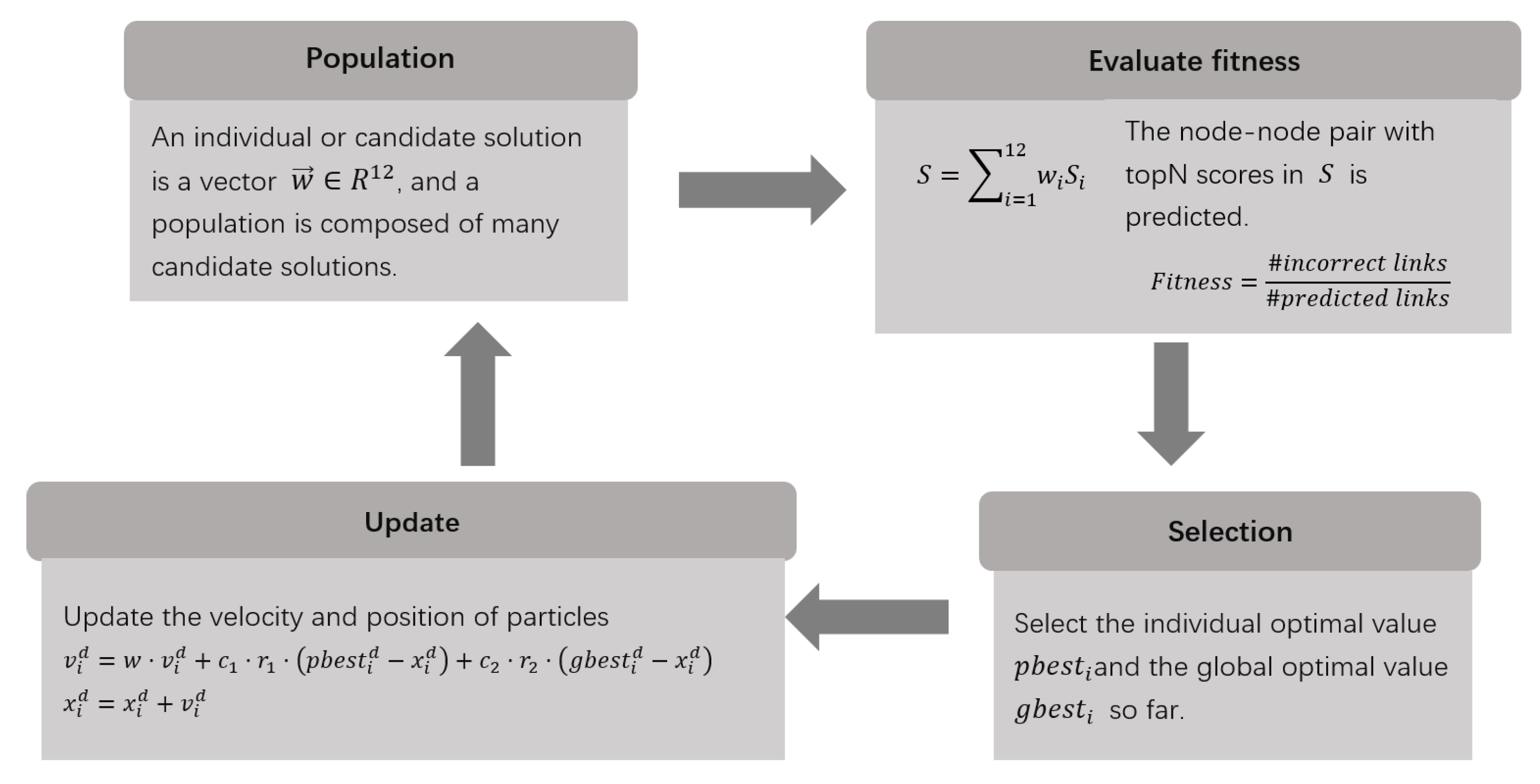
Figure 2 roughly describes the process of link prediction using particle swarm optimization. Before using the algorithm, we calculated all the topological similarity index values and stored them in the $N\times N$ sparse matrix $S_i$, $i=1,2,\dots ,12$, and N is the number of author nodes in the academic social network here. This process is actually to get all the similarity index value data corresponding to every node pair. The similarity indices are linearly combined according to the method shown in Formula (3), and the coefficient $w_i$ is updated by the evolution of the particle swarm algorithm which means $\overrightarrow{w}$ is actually equal to the position vector of a particle. The initial value of $w_i$ is randomly selected from 0 to 1.

$$S=\sum _{i=1}^{12}{w}_i{S}_i$$

(3)

In each iteration, the node–node pair corresponding to the topN values of the score ranking in S is considered as our predicted link. The aim of our algorithm is to find the best $\overrightarrow{w}$ so far within a limited number of iterations that maximizes the proportion of correctly predicted links in the predicted links. By comparing the predicted link with the link appearing in the next year, incorrect links can be obtained. As shown in Formula (4), we take the fitness value as the ratio of the number of incorrect links to the number of predicted links. Since the number of predicted links is constant topN, the fitness value is proportional to the number of incorrectly predicted links, that is, inversely proportional to the number of correctly predicted links. When the fitness value is equal to 0, the number of incorrect links is also equal to 0, that is, all predicted links are correctly predicted links, which is the ideal result we most want to see. Therefore, each iteration can find the optimal particle in the population that can make the fitness reach the smallest in history, and it will enter the next iteration. In our algorithm, when the maximum number of iterations is reached, or the historically optimal particle can satisfy the condition that the fitness value is 0 in advance, the iteration stops.

3.4. Spark Implementation of Particle Swarm Algorithm

The complete pseudocode of Spark is shown in Algorithms 1–3. Algorithm 1 is the main program running on the Driver side. Before starting, the data file that needs to be used is loaded into RDD through the textFile method of Spark, and the RDD is then converted appropriately. The sparseMatrixRDD and testRDD are in the form of key–value pairs, and considering that the program needs to use them every time the fitness value is calculated, we used Spark’s persist method (line 2) to persist these two RDDs in memory for later use, and SparseMatrixRDD will use the partitionBy method to perform the Hash partition operation before this operation. Next, we randomly initialized a particle group RDD particlesPreRDD without a fitness value attribute by calling Spark’s parallelize method and map method, and then called Algorithm 2 to calculate the fitness value of the initialized particles and the best fitness value of the individual (line 5). We obtained the particle group RDD particlesRDD used in the iterative loop (line 6), and then used the best individual gbTemp in the current initial particle group as the global historical best individual gb temporarily (line 8). When the upper limit of the iteration is not met, in each iteration loop, all particles and the best particles will be broadcast down (line 10, 11), and then Algorithm 3 will be called to update the speed and position in the particle column. The best position and the best fitness value of the individual were also adjusted accordingly according to the situation, and the best individual gbTemp (line 13) in the current particle swarm after the update was found again. If it is better than the recorded global history best individual gb, gbTemp was used to update gb (line 14, 15).

$$Fitness=\frac{\#incorrectlinks}{\#predictedlinks}$$

(4)

In our link prediction for academic paper collaborators, since the dimension of $\overrightarrow{w}$ needs to be equal to the number of similarity indices, that is, the particle dimension is 12, we set the population size to this value for convenience in the experiment. The population is small and the amount of data is huge. The most time-consuming part of the particle swarm algorithm is the calculation of the fitness value. Therefore, how parallel calculations should be performed when evaluating the fitness value of the particle swarm algorithm implemented by Spark becomes a key consideration. In Algorithm 3, before calculating the fitness value, you must first obtain the predicted link. This requires certain operations on the key–value pair RDD sparseMatrixRDD (line 2) that has been divided into areas. First, the mapValue method is used in Spark to perform a separate operation on the value. For operation, the product sum of each similarity index corresponding to the link and each dimension value of $\overrightarrow{w}$ (that is, each dimension value of the particle position vector) was obtained, and this product sum was used as a score for judging whether a link is a predicted link. Due to the huge amount of data, in order to avoid the use of sortByKey and other shuffle-related operators as much as possible, and successfully extract TopN in hundreds of millions of data, we used mapPartition to find the smallest heap in each partition, and then used flatMap to summarize each partition first. The minimum heap set data is then the smallest heap. After flattening, the RDD key was taken to get the predicted link RDD predictRDD. After that, the predicted link was compared with the test link, and the fitness value could be easily calculated.

Algorithm 1 Spark-PSO Algorithm

Input:  populationSize, maxIteration, dimension, dataset Output:  the best solution  1: topNBC <- sc.broadcast(topN)  2: Load data and transform the loaded data RDD as Key-value pair RDD: sparseMatrixRDD((fromNodeID, toNodeID), (J, A, C, P, K, Pr, R, Hp, Hd, L, Sa, So)) and testRDD(fromAuthorID, toAuthorID), then Hash partition sparseMatrixRDD and persist the two RDD into memory.  3: Generate a randomly initialized population as particlesPreRDD in the format (particleID, position, velocity, pbest)  4: particlesPreArray <- particlesPreRDD.collect  5: Add fitness and pbFitness for every element in particlesPreArray using Algorithm 2 and get particlesArray with particles in the format (ID, position, velocity, fitness, pbest, pbFitness)  6: particlesRDD <- sc.parallelize(particlesArray)  7: gbTemp <- particlesRDD.sortBy((._4, true)).take(1)(0)  8: gb <- gbTemp  9: while t < maxIteration do  10:    gbBC<-sc.broadcast(gb)  11:    particlesBC <- sc.broadcast(particlesArray)  12:    Update every particle in particlesArray using Algorithm 3  13:    gbTemp <- particlesRDD.sortBy((._4, true)).take(1)(0)  14:    if gbTemp._2 < gb._2 then  15:      gb = gbTemp  16:    end if  17:    particlesRDD <- sc.parallelize(particlesArray)  18:    gbBC.destroy  19:    particlesBC.destroy  20:    t = t + 1  21: end while  22: topNBC.destroy  23: Output gb._2(gbest) as the best solution

Algorithm 2 calculateFitness Algorithm

Input:  position, sparseMatrixRDD, testRDD, topNBC Output:  fitness  1: finalHeap < PriorityQueue.empty(MinOrder)  2: predictRDD <- sparseMatrixRDD.mapValues(tuple1=>${\sum }_{i=0}^{11}$(tuple1._(i + 1)*position(i)))  .mapPartitions(iterator=>{    minHeap<-PriorityQueue.empty(MinOrder)    iterator.foreach(tuple2=>{       minHeap.enqueue(tuple2)       if minHeap.length > topNBC.value             minHeap.dequeue()       end if       minHeap}    minHeap.toIterator    }).flatMap(tuple3=>{       finalHeap.enqueue(tuple3)       if finalHeap.length >topNBC.value             finalHeap.dequeue()       end if       finalHeap}).map(_._1)  3: incorrectNum <- topN-predictRDD.intersection(testRDD).count  4: fitness <- 1.0 * incorrectNum/topN  5: return fitness

Algorithm 3 updateParticle Algorithm

Input:  partcle,gbest,sparseMatrixRDD, testRDD, topNBC Output:  particle  1: Update velocity and position according to Formulas (1) and (2)  2: Evaluate fitness using Algorithm refa2  3: if fitness < pbFitness then  4:    set current particle to pbest  5: end if  6: return particle

4. Experiment and Result Analysis

Experimental Evaluation Methods and Results

Figure 3 shows the fitness20 (topN = 20) results of new links formed during the training period from 1986 to 1987. The black solid line depicting the “Topo12” predictor shows that the average optimal fitness value of 100 candidate solutions dropped sharply from 0.7505 to 0.0475 within 10 generations, and then eased slightly, and dropped to 0.006 by the 27th generation. In the 50th generation, it was reduced to 0.0025. After that, the line was getting closer and closer to the X-axis. By the 87th generation, it completely coincided with the X-axis, and the average optimal fitness value reached a satisfactory result of 0. The curves are consistent with the characteristics that the particle swarm optimization algorithm converges quickly at the beginning of the iteration and slowly at the end, and the overall convergence is relatively fast. In fact, the optimal fitness value converges to 0 much earlier in most runs, but the image depicts the average result over 100 runs, and because the particle swarm algorithm has the disadvantage of easily falling into local optima late in the process, several of these runs take far more generations than normal to reach a fitness value of 0, thus lengthening the number of generations required for the overall average.

To better understand the performance of each topological similarity index in the employed link predictor, we plotted Figure 4 to visualize this aspect of information. Figure 4 shows all 100 solutions obtained by evolving the particle swarm optimization algorithm in parallel with Spark for 250 generations, where $\overrightarrow{w}$ is used as the horizontal row. The i-th column represents the coefficients of $w_i$ used for the linear combination, and the color of the axes indicates the position where the coefficient values are located. It can be observed from the images that the 100 candidate solutions differ significantly from each other. Nevertheless, we can still find more positive than negative values for the Average Path Weight and Katz, with the former accounting for more than 90% of the positive values and the latter not even having any negative values, while Preferential Attachment is basically all negative with only two sporadic positive values. This means that for a high-scoring author pair, if it contains a large number of positive weights for Average Path Weight and Katz and a large number of negative weights for Preferential Attachment, then a link between the two authors will be more likely to be generated in the future, that is, more likely to collaborate.

The ranking frequencies of each similarity index were visualized according to their coefficients, as shown in Figure 5. The coefficients are ordered from the most positive (in first place) to the most negative (in 12th place). As can be seen from the images, Average Path Weight and Katz frequently occupy the first to fourth positions in the ranking, while the Hub-promoted Index, Hub-depressed Index, Leicht-Holme-Newman Index, Salton Index, and Sorenson Index ranked 8th to 12th most frequently. The other indices were relatively dispersed.

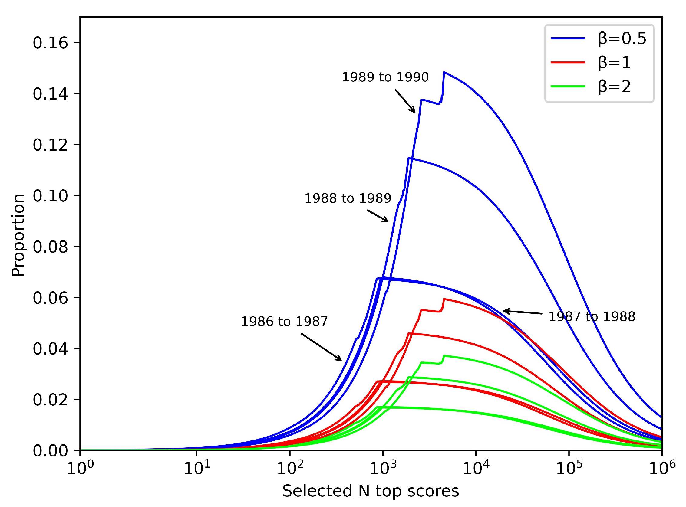
Since the positive class is much smaller than the negative class in large sparse networks, given this imbalance, even for random link predictors, metrics such as accuracy and negative predictive value are very close to 1. Therefore, this paper puts more attention on recall and accuracy, which are shown in Equations (5) and (6), respectively, and Equation (7) is a combined metric $F_{\beta }$ that combines the two.

$$\mathrm{recall}=\frac{TP}{TP+FN}$$

(5)

$$\mathrm{precision}=\frac{TP}{TP+FP}$$

(6)

$$F_{\beta }=(1+{\beta }^2)·\frac{\mathrm{precision}·\mathrm{recall}}{({\beta }^2·\mathrm{precision})+\mathrm{recall}}$$

(7)

$\beta$ is used to adjust the weight of recall and accuracy—when $\beta =1$ both weights are the same, if the accuracy is considered more important then $\beta$ is reduced, and if recall is considered more important then $\beta$ is increased accordingly.

Adjusting $\beta$ to one of 0.5, 1, and 2, respectively and plotting Figure 6, it is easy to find that $F_1$ reaches its extreme value roughly at $N\approx {10}^3$. Since the number of selected academic network collaborator nodes increases with the year, the corresponding number of node–node pairs of links consisting of any two authors also increases with the year with a difference of hundreds of millions or more. It is observed that for years with a higher number of links, the $F_{\beta }$ value is also clearly higher.

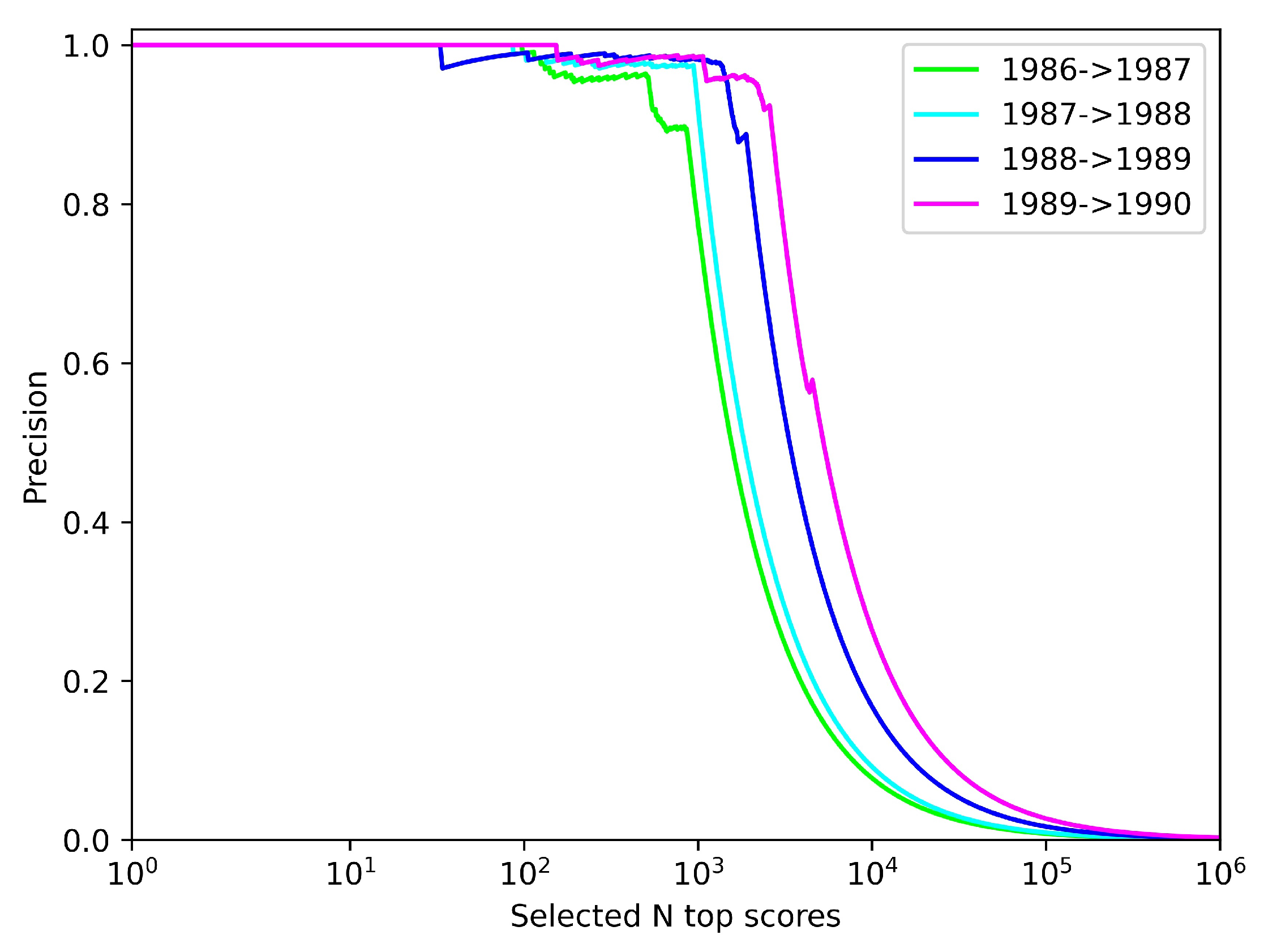
Figure 7 depicts the precision of the link prediction under the top N-scoring author–author pairs. It is not difficult to find that the fitness function of the algorithm runs achieves essentially zero-error precision across the validation sets when scoring author–author pairs below about ${10}^2$ are selected, and extremely high precision between ${10}^2$ and ${10}^3$. After that, the curve plummets from smallest to largest by validation set year, mainly because all correctly predicted links have been basically identified until N is about ${10}^3$, and increasing N further just increases the false-positive rate in vain. Overall, it can be seen that our prediction of co-authorship works well.

5. Summary and Outlook

In big data research, the problem of link prediction in social networks has always been an important area. In this article, we use the Apache Spark framework to design and implement a parallel particle swarm optimization link prediction algorithm for the first successful prediction of academic paper cooperation relationships. By paying more attention to the design and parallel computing of fitness evaluation, our algorithm adapted to the task of big data processing well. We conducted convincing experiments for the proposed algorithm on the real academic paper collaborator data set. We drew a graph of the average convergence of fitness values, and indirectly observed the performance of each similarity index through the range and ranking of the best $\overrightarrow{w}$ dimension values, and used the evaluation indicators precision and $F_{\beta }$ on four validation sets to further observe the prediction effect. The design experiment observation also shows that the link prediction effect of our method is obviously better than papers simply choosing serial intelligent optimization algorithms or simply using a big data framework without adjusting the fitness calculation to suit the real big data applications, which illustrates the effectiveness of the particle swarm optimization algorithm and the high adaptability of Spark to iteratively process large-scale data even when the population is small. In future work, we suggest using improved variants of particle swarm algorithm or other swarm intelligence optimization algorithms for link prediction or application in other real big data instances, which may have more different gains.

References

- Kennedy, J.; Eberhart, R. Particle swarm optimization. In Proceedings of the ICNN’95—International Conference on Neural Networks, Perth, WA, Australia, 27 November–1 December 1995; Volume 4, pp. 1942–1948. [Google Scholar]
- Shi, Y. Particle swarm optimization: Developments, applications and resources. In Proceedings of the 2001 Congress on Evolutionary Computation, Seoul, Korea, 27–30 May 2001; Volume 1, pp. 81–86. [Google Scholar]
- Snir, M.; Gropp, W.; Otto, S.; Huss-Lederman, S.; Dongarra, J.; Walker, D. MPI–The Complete Reference: The MPI Core; MIT Press: Cambridg, MA, USA, 1998. [Google Scholar]
- Dean, J.; Ghemawat, S. MapReduce: Simplified data processing on large clusters. Commun. ACM 2008, 51, 107–113. [Google Scholar] [CrossRef]
- McNabb, A.W.; Monson, C.K.; Seppi, K.D. Parallel pso using mapreduce. In Proceedings of the 2007 IEEE Congress on Evolutionary Computation, Singapore, 25–28 September 2007; pp. 7–14. [Google Scholar]
- Sadasivam, G.S.; Selvaraj, D. A novel parallel hybrid PSO-GA using MapReduce to schedule jobs in Hadoop data grids. In Proceedings of the 2010 Second World Congress on Nature and Biologically Inspired Computing (NaBIC), Kitakyushu, Japan, 15–17 December 2010; pp. 377–382. [Google Scholar]
- Wang, J.; Yuan, D.; Jiang, M. Parallel k-pso based on mapreduce. In Proceedings of the 2012 IEEE 14th International Conference on Communication Technology, Chengdu, China, 9–11 November 2012; pp. 1203–1208. [Google Scholar]
- Zaharia, M.; Xin, R.S.; Wendell, P.; Das, T.; Armbrust, M.; Dave, A.; Meng, X.; Rosen, J.; Venkataraman, S.; Franklin, M.J.; et al. Apache spark: A unified engine for big data processing. Commun. ACM 2016, 59, 56–65. [Google Scholar] [CrossRef]
- Guo, X.; Chen, S.; Zhang, Y.; Li, W. Service composition optimization method based on parallel particle swarm algorithm on spark. Secur. Commun. Netw. 2017, 2017, 9097616. [Google Scholar] [CrossRef] [Green Version]
- Duan, Q.; Sun, L.; Shi, Y. Spark clustering computing platform based parallel particle swarm optimizers for computationally expensive global optimization. In Proceedings of the International Conference on Parallel Problem Solving from Nature, Coimbra, Portugal, 8–12 September 2018; Springer: Cham, Switzerland, 2018; pp. 424–435. [Google Scholar]
- Zhang, W.; Huang, Y. Using big data computing framework and parallelized PSO algorithm to construct the reservoir dispatching rule optimization. Soft. Comput. 2020, 24, 8113–8124. [Google Scholar] [CrossRef]
- Sherar, M.; Zulkernine, F. Particle swarm optimization for large-scale clustering on apache spark. In Proceedings of the 2017 IEEE Symposium Series on Computational Intelligence (SSCI), Honolulu, HI, USA, 27 November–1 December 2017; pp. 1–8. [Google Scholar]
- Al-Sawwa, J.; Ludwig, S.A. Parallel particle swarm optimization classification algorithm variant implemented with Apache Spark. Concurr. Comp-Pract. E 2020, 32, e5451. [Google Scholar] [CrossRef]
- Bliss, C.A.; Frank, M.R.; Danforth, C.M.; Dodds, P.S. An evolutionary algorithm approach to link prediction in dynamic social networks. J. Comput. Sci. 2014, 5, 750–764. [Google Scholar] [CrossRef] [Green Version]
- Karau, H.; Konwinski, A.; Wendell, P.; Zaharia, M. Learning Spark: Lightning-Fast Big Data Analysis; O’Reilly Media, Inc.: Newton, MA, USA, 2015. [Google Scholar]
- Li, Y.; Chen, Z.; Wang, Y.; Jiao, L. Quantum-behaved particle swarm optimization using mapreduce. In Proceedings of the International Conference on Bio-Inspired Computing: Theories and Applications, Xi’an, China, 28–30 October 2016; Springer: Singapore, 2016; pp. 173–178. [Google Scholar]
- Aljarah, I.; Ludwig, S.A. Mapreduce intrusion detection system based on a particle swarm optimization clustering algorithm. In Proceedings of the 2013 IEEE Congress on Evolutionary Computation, Cancun, Mexico, 20–23 June 2013; pp. 955–962. [Google Scholar]
- Aljarah, I.; Ludwig, S.A. Towards a scalable intrusion detection system based on parallel pso clustering using mapreduce. In Proceedings of the 15th Annual Conference Companion on Genetic and Evolutionary Computation, Amsterdam, The Netherlands, 6–10 July 2013; ACM: New York, NY, USA, 2013; pp. 169–170. [Google Scholar]
- Chunne, A.P.; Chandrasekhar, U.; Malhotra, C. Real time clustering of tweets using adaptive PSO technique and MapReduce. In Proceedings of the 2015 Global Conference on Communication Technologies (GCCT), Thuckalay, India, 23–24 April 2015; pp. 452–457. [Google Scholar]
- Xu, Y.; You, T. Minimizing thermal residual stresses in ceramic matrix composites by using Iterative MapReduce guided particle swarm optimization algorithm. Compos. Struct. 2013, 99, 388–396. [Google Scholar] [CrossRef]
- Sherkat, E.; Rahgozar, M.; Asadpour, M. Structural link prediction based on ant colony approach in social networks. Phys. Stat. Mech. Appl. 2015, 419, 80–94. [Google Scholar] [CrossRef]
- Barham, R.; Aljarah, I. Link prediction based on whale optimization algorithm. In Proceedings of the 2017 International Conference on New Trends in Computing Sciences (ICTCS), Amman, Jordan, 11–13 October 2017; pp. 55–60. [Google Scholar]
- Shi, Z.; Zuo, W.; Chen, W.; Yue, L.; Han, J.; Feng, L. User relation prediction based on matrix factorization and hybrid particle swarm optimization. In Proceedings of the 26th International Conference on World Wide Web Companion, Perth, Australia, 3–7 April 2017; pp. 1335–1341. [Google Scholar]
- Zhuang, H.; Sun, Y.; Tang, J.; Zhang, J.; Sun, X. Influence maximization in dynamic social networks. In Proceedings of the 2013 IEEE 13th International Conference on Data Mining, Dallas, TX, USA, 7–10 December 2013; pp. 1313–1318. [Google Scholar]
Figure 1.
Network topology of the platform.
Figure 2.
Spark-PSO link prediction process.
Figure 3.
Average best fitness (average gbFitness) calculated from 100 simulations of PSO for training new links appearing in 1987.
Figure 4.
The 100 best individuals evolved from pso (from top to bottom, there are 1~100 rows, and each row represents a best individual).
Figure 5.
The frequency graph drawn by the ranking coefficient, where corresponds to the similarity index.
Figure 6.
of link prediction in each validation set.
Figure 7.
Precision of link prediction in each validation set.